On the Nitrous Oxide Accumulation in Intermediate Waters of the Eastern South Pacific Ocean

Introduction

Approximately 90% of the total marine nitrous oxide (N₂O) inventory occurs between depths just below the pycnocline down to ~1000 m (Nevison et al., 1995, 2003; Suntharalingam and Sarmiento, 2000). Nitrification and denitrification are the principal processes involved in N₂O production. Both processes depend on organic matter availability and oxygen (O₂) levels, but whereas the former occurs under a wide range of oxygen conditions, the latter takes place only at suboxic and anoxic levels (Codispoti et al., 2001; Bange, 2008). Coastal upwelling systems with high primary production (PP) rates meet both these conditions for enhanced N₂O production (Nevison et al., 2004) and are closely linked to Oxygen Minimum Zones (OMZs). The formation/maintenance of OMZs is predominantly determined due to slow ventilation; while high aerobic respiration of particulate organic matter (POM) is probably of second importance (Karstensen et al., 2008).

N₂O production by nitrification; i.e., the aerobic oxidation of ammonium (${\text{NH}}_4^{+}$) to nitrite (${\text{NO}}_2^{-}$), and then to nitrate (${\text{NO}}_3^{-}$), is controlled by O₂ concentration. An increased N₂O yield is triggered by lower concentrations of O₂ (Goreau et al., 1980) and previous studies have shown that significant quantities of N₂O are produced by Bacteria and Archaea at O₂ concentrations below 5 μmol L⁻¹ (Frame and Casciotti, 2010; Santoro et al., 2011; Löscher et al., 2012). In addition, in a process known as nitrifier denitrification, autotrophic ${\text{NH}}_4^{+}$ oxidizing bacteria are able to produce N₂O as a final product of ${\text{NO}}_2^{-}$ reduction (Poth and Focht, 1985). In contrast, denitrification, the process by which ${\text{NO}}_3^{-}$ is reduced to produce N₂ gas as final end product and N₂O as an intermediate, only occurs at O₂levels close to anoxia (Dalsgaard et al., 2014).

Very limited information is available regarding N₂O production in intermediate waters, approximately between 500 and 1200 m depth, (Suntharalingam and Sarmiento, 2000; Nevison et al., 2003; Freing et al., 2012), with several of these studies carried out in the eastern tropical North Pacific and the Arabian Sea (Naqvi and Noronha, 1991; Bange et al., 2005; Yamagishi et al., 2007; Fujii et al., 2013). The intermediate depths of the eastern South Pacific (ESP) are occupied by two water masses that move in opposite directions and mix as they converge, i.e., Equatorial Subsurface Water (ESSW) and Antarctic Intermediate Water (AAIW). The AAIW is formed along the front of the Antarctic Circumpolar Current (Sverdrup et al., 1942; McCartney, 1977; Talley, 1999) and spreads equatorward along the lower boundary of the thermocline, in a core layer with a potential density (σ_θ) of about 27.0–27.1 kg m⁻³ (AAIWσ_θ). AAIW also has low outcrop temperatures and salinities, and therefore, a high capacity for storing dissolved gases (Georgi, 1979). Unlike AAIW, the ESSW is the end product of complex water mass transformations of different sources within the equatorial belt (Wyrtki, 1963, 1967; Tsuchiya and Talley, 1996; Fiedler and Talley, 2006). Being a product of mixing, the bulk of the contributing water masses that compose ESSW have a long residence times of at least several decades (Kessler, 2006), and ESSW is immediately identifiable by comparably very low O₂ levels, relative to AAIW.

Given the contrasting histories of these two water masses, taking into consideration their relative mixing properties is fundamental when interpreting biogeochemical fields in the ESP (Llanillo et al., 2013). Optimum Multiparameter (OMP) analysis (Tomczak and Large, 1989; Karstensen and Tomczak, 1998) is a tool that enables the separation between water mass mixing and bulk biogeochemical cycling. OMP analysis solves for linear mixing of source waters and time integrated modifications by biogeochemical cycling processes (Karstensen and Tomczak, 1998; Hupe and Kartsensen, 2000). For biogeochemical cycling, the analysis resolves the inverse co-variability between oxidation (reduction of oxygen) and remineralization (release of dissolved nutrients) according to a prescribed Redfield ratio. Water masses originating from different source regions are impacted by different biogeochemical modifications en route before they meet and mix. The mixing in turn can generate local apparent non-linearity in biogeochemical ratios, as shown by Schneider et al. (2005). These authors analyzed the output of a physical/biogeochemical model run with a constant Redfield ratio. Following this approach, we separated the mixing signal from the biogeochemical signal in the ESP, in order to estimate N₂O production in intermediate waters. Several approaches have been used to estimate water age and the consequent accumulation of N₂O over time, among them, Bange and Andreae (1999) calculated an annual global N₂O accumulation in deep waters using the age estimate provided by Broecker et al. (1988) with the radiocarbon methods. Freing et al. (2009, 2012) estimated N₂O production rates by using the transient time distribution (TTD) approach, which provides age estimation using tracers, such as chlorofluorocarbon (CFC-12) and sulfur hexafluoride (SF₆). Here, we estimated the water mass age using chlorofluorocarbon (CFC-11) data from the World Ocean Circulation Experiment (WOCE). We also analyzed relationships between biogeochemical parameters as apparent N₂O production (ΔN₂O) with apparent oxygen utilization (AOU), ${\text{NO}}_3^{-}$, ${\text{NO}}_2^{-}$, and N* (a quasi-conservative tracer, defined as a linear combination of nitrate and phosphate, Gruber and Sarmiento, 1997) to estimate the origin of N₂O in AAIW.

Methods

Hydrographic Data

Observational data was used from a total of 14 cruises between 10° and 60°S, and off the coast of South America to 88°W (Figure 1, Table 1). Data were compiled from several cruises (Table 1): (1–4) the World Ocean Circulation Experiment (WOCE, United States) transects P19C, P19S, P21E, and P06E, with CFC measurements; (5) the Sonne 102 cruise; (6) the CIMAR 5 cruise (Servicio Hidrografico y Oceanografico de la Armada de Chile, SHOA); (7) the German DFG collaborative research project (SFB) 754 (M77-4 cruise, Germany); (8) the SubAntarctic Mixed Layers, Fluxes, and Overturning Circulation project (SAMFLOC); (9) the Japanese Agency for Marine-Earth Science and Technology (JAMSTEC); (10) the Danish Galathea 3 Expedition; (11) the Biogeochemistry and Optics South Pacific Experiment (BIOSOPE); (12) the Fondo de Investigación Pesquera (FIP 2006 cruise, Chile); (13) the WHOI project (KN 182-9 cruise); and (14) the Center for Microbial Oceanography: Research and Education (C-MORE, Big-Rapa cruise). The different Conductivity-Temperature-Depth (CTD) models used and the respective calibrations are described in subsequent reports to the respective cruises, and indicate that temperature can be considered accurate to 0.005 K and salinity to 0.005 PSS-78.

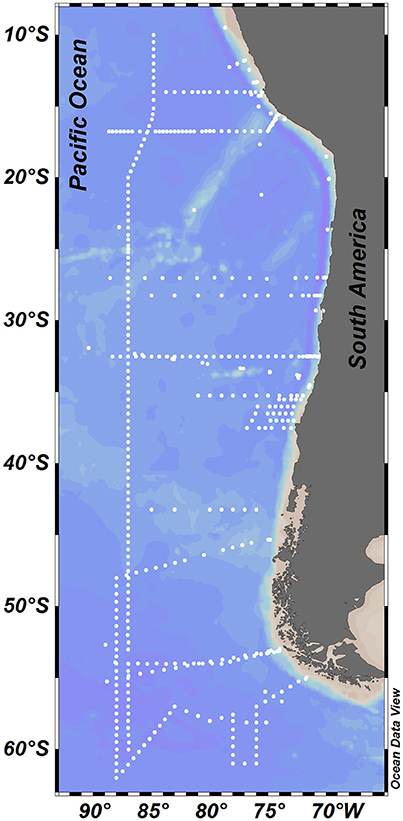
Figure 1. Study area showing the station locations where physical and biogeochemical measurements were taken.

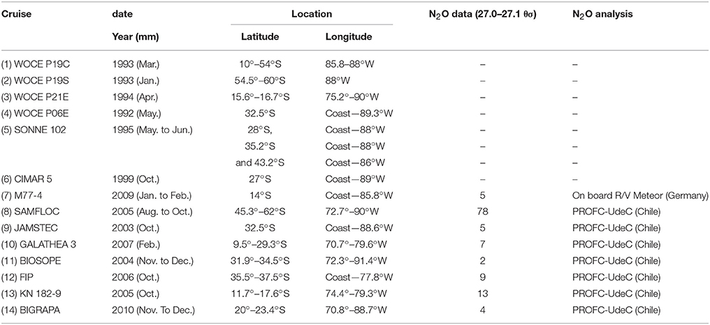
Table 1. Locations and dates of the cruises, including N₂O data compiled in this study.

Chemical Analysis

Measurements of dissolved N₂O were taken during eight cruises (Table 1). Here, we describe N₂O analysis from the Laboratory of Oceanographic Processes and Climate (PROFC-UdeC, Chile). N₂O samples were taken in triplicate in 20 mL vials and carefully sealed to avoid air bubbles. They were then preserved with 50 μL of saturated HgCl₂ and stored in darkness until analysis. N₂O was analyzed by creating a 5 mL headspace of ultrapure He and then equilibrated within the vial, and measured with a gas chromatogram (Shimadzu 17A) using an electron capture detector (ECD). The calibration curves were made previous to each measurement with five points using pure Helium, 0.1, 0.5, and 1 of N₂O standards and dry air. The ECD detector linearly responded to this concentration range and the analytical error for N₂O measurements was ~3%. The uncertainty of the measurements was calculated from the standard deviation of the triplicate measurements by depth. Samples with a variation coefficient above 10% were not considered in the N₂O database. N₂O analyses from the M77-4 cruise are described in Kock et al. (2016). Oxygen and nutrient data, including descriptions of O₂ sensors used on CTD-O instruments (where applicable), are described in subsequent reports to the respective cruises. During the Galathea 3 cruise (Table 1), an ultrasensitive STOX O₂ sensor was tested, which allowed an O₂ detection limit of 1–10 nmol L⁻¹ (Revsbech et al., 2009).

Data Analysis

Classical Approach

N₂O accumulation rates throughout the AAIW core were estimated by determining the differences in concentration between two latitudes, and considering an estimated AAIW age. Age was derived using a standard procedure, which in brief involves converting observed CFC-11 into its atmospheric equivalent with the aid of the CFC-11 solubility function (Warner and Weiss, 1985), and this is then compared to the historical atmospheric time series data (Walker et al., 2000), resulting in an estimate of the “year of last atmospheric contact.” The difference between the year of observation and the year of last atmospheric contact is interpreted as water age. This method has many uncertainties, including the CFC-11 saturation value in uptake regions (here assumed to be 100%), and particularly the impact of mixing with waters of different ages (Waugh et al., 2003). CFC-11 is a tracer that was introduced into the atmosphere in the 1950's–1960's, and thus cannot be used to determine water masses formed before that date, which is a potential problem in OMZ regions (Karstensen et al., 2008). Because age determination of the water mass in the OMZ has several associated anomalies due to slow circulation, we try to minimize uncertainty by only calculating ages for the lower thermocline, south of 16°S.

Due to the spatial distribution of data, and the relative paucity of observations, it is not possible to determine systematic temporal changes; however comparison of data located in similar positions feature the same trend (not shown). We are confident that despite some variability exists in the data due to time of analysis the main oceanic conditions prevailed among years.

On the other hand, because the data used belong to different years, data variability due to oscillation in the global ocean/atmosphere system as ENSO (El Niño/Southern Oscillation) may occur. ENSO is a periodic fluctuation in sea surface temperature (El Niño) and the air pressure of the overlying atmosphere (Southern Oscillation) across the equatorial Pacific Ocean. The fluctuations in sea surface temperature oscillate between two states: El Niño phase, with warmer than normal temperatures and La Niña phase with cooler than normal temperatures. Llanillo et al. (2013) examined the changes in the water mass structure and biogeochemical signals of two opposite phases of ENSO (El Niño and La Niña) in the eastern tropical South Pacific in 1993 and 2009. They found the largest ENSO impact in the water properties and water mass distribution in the upper 200 m north of 10°S with the result of the vertical motion of the oxygen minimum zone (OMZ). During El Niño event (warm phase), there was increased advection of relatively well-oxygenated Subtropical Surface Water (STW) which replaced the low-oxygen ESSW in the top 250 m of the water column. This input deepened the upper part of the OMZ. In contrast, during the 2009 La Niña conditions, the reinforced trade winds drove enhanced upwelling, raising the upper part of the OMZ.

According to the Oceanic Niño Index (ONI), one of the primary indices used to monitor ENSO, conditions for El Niño (weak to moderate) predominated in the period analyzed (from 1992 to 2010, http://www.cpc.ncep.noaa.gov/products/analysis_monitoring/ensostuff/ensoyears.shtml). We do not have data during the years 1996–1998, in which it was developed one of the most intense El Niño episodes.

Delta, or excess of N₂O (ΔN₂O), is a measure of the apparent production of N₂O (Nevison et al., 1995), and was calculated as ΔN₂O = [N₂O]_{in situ} − [N₂O]_eq, where [N₂O]_{in situ} is the measured concentration of N₂O, and [N₂O]_eq is the concentration of N₂O in saturation with the atmosphere at the time of the last atmospheric contact (provided by the CFC-11 age; Weiss and Price, 1980). Given its recent ventilation and uptake capacity (low temperatures), we expect AAIW to be affected by the anthropogenic increase in the N₂O atmospheric mixing ratio, and an atmospheric mole fraction was estimated for the time of the last atmospheric contact. The atmospheric concentration during the year of formation was derived from the slope of N₂O increase per year (Machida et al., 1995; http://www.esrl.noaa.gov/gmd/hats/combined/N2O, NOAA/ESRL program). Apparent Oxygen Utilization (AOU) was calculated as the difference between the equilibrium concentration (Garcia and Gordon, 1992) and observed O₂. Finally, correlations of ΔN₂O vs. AOU; ${\text{NO}}_3^{-}$: ${\text{NO}}_2^{-}$ and N*, along AAIWσ_θ were made through least square fit with Ocean Data View (ODV) program.

Mixing Analysis Approach

In order to distinguish inner ocean N₂O modifications due to the mixing of water masses with differences in source values, we applied the OMP analysis (http://omp.geomar.de). First, the source water characteristics for the ESP were defined on the basis of previous studies (De Pol-Holz et al., 2007; Silva et al., 2009; Llanillo et al., 2013), but also taking into consideration the data at hand. The source water characteristics used in this study are presented in Table 2. As seen from source water types, ESSW and AAIW are very different, the former being a mixture of multiple sources and low in O₂ but high in N₂O; while the latter is close to saturation in both O₂ and N₂O. For every single observational data point, a solution vector was derived using a non-negative least squares fit, and the outputs of the analysis were presented as water mass fractions and total amount of biogeochemical modifications. The fraction range was between 0 (no contributions of a specific water mass) and 1 (exclusive contribution of a specific water mass), and was then converted to 0–100%. The connection between nutrients and oxygen is established by using a fixed elementary ratio (Anderson and Sarmiento, 1994). Varying this ratio did not significantly impact the results (Hupe and Kartsensen, 2000).

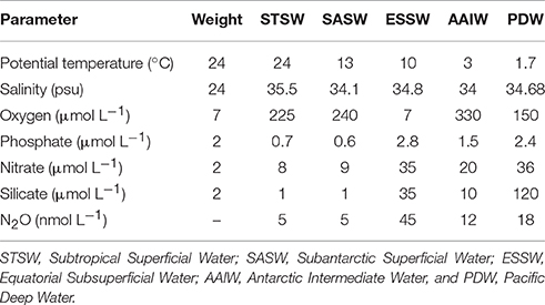
Table 2. Physical and biogeochemical variables and weights of source water types used for Optimum Multiparameter analysis (OMP).

Results and Discussion

The distribution of physical (temperature and salinity) and biogeochemical (O₂ and N₂O) variables within ESP nicely depicts the water mass structure for the intermediate depth range of the ESP (Figure 2). The AAIW can be identified by its low temperature/high O₂ content, emanating as a tongue out of a core depth of about 600 m from about 60°S toward the equator, along a potential density of 27.1 kg m⁻³ (Figures 2B,C). The ESSW core spread along the 26.6 kg m⁻³ isopycnal and is seen as a core of low O₂/high salinity water (Figures 2C,D). During its northward propagation, the AAIW core density gets warmer (3.0–8.0° C) and saltier (<34–34.6).

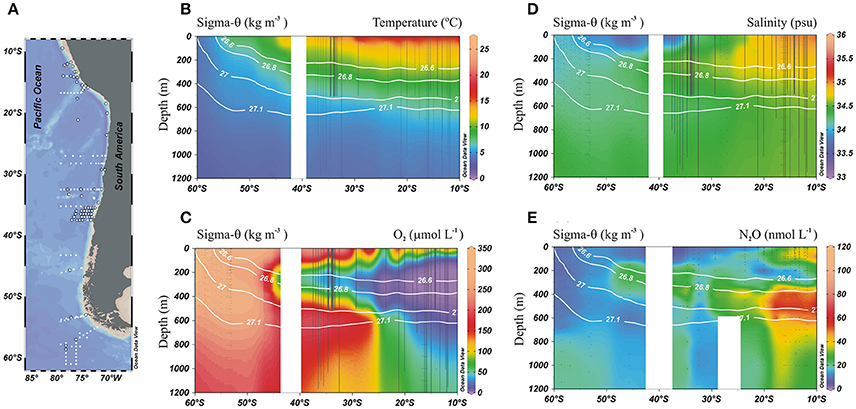
Figure 2. Physical and biogeochemical distributions in the meridional section of the eastern South Pacific: (A) Station locations, (o) indicates profiles with N₂O data; (B) Temperature (°C); (C) O₂ (μmol L⁻¹); (D) Salinity (psu), and (E) N₂O (nmol L⁻¹). Black dots indicate sampling stations at depth and white lines denote potential density isolines (kg m⁻³).

The presence of the OMZ is seen from depleted O₂ levels (<22 μmoL L⁻¹, Figure 2C), between 100 and 400 m and north of 30°S. Lowest O₂-values, possibly reaching anoxia (<1 μmol L⁻¹), have been reported off Peru and northern Chile at shallow depths ~100–300 m (Canfield et al., 2010). At the AAIW core (27–27.1 kg m⁻³; Figure 3), dissolved O₂ decreased from 325 to 58 μmol L⁻¹ (from 97 to 19% saturation), between 60° and 20°S (Figure 3A). In contrast, N₂O concentrations were lowest at high latitudes (close to the AAIW source region), with a value of 8 nmol L⁻¹ (68% saturation) at 58°S and gradually increasing to more than 26 nmol L⁻¹ (231% saturation) at 20°S (Figure 3B). Further north, O₂ levels fall drastically down to 0.12 μmol L⁻¹ or 4% saturation (minimum value recorded) at 12°S (Figure 3A); while N₂O at this O₂ concentration is 47 nmol L⁻¹ (412% saturation). Interestingly, this is not the maximum value of N₂O. The maximum found was 75 nmol L⁻¹ (657% saturation) at an O₂ concentration of 25 μmol L⁻¹ (8% saturation) at 17.6°S (Figure 3B). The greatest N₂O accumulation was found between the core waters of ESSW and AAIW at the 26.8 kg m⁻³ isopycnal, with concentrations of up to 87 nmol L⁻¹ at 13°S (Figure 4). This indicates favorable conditions for local N₂O production.

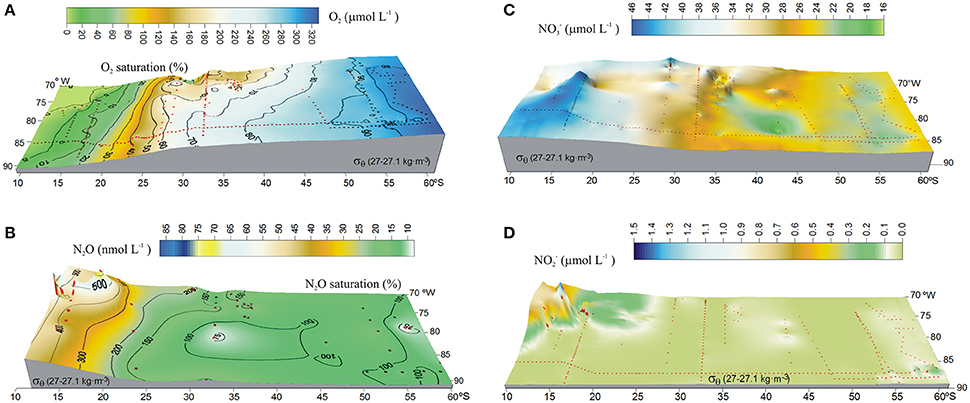
Figure 3. Isopycnal surface distribution along 27–27.1 kg m⁻³ (AAIW) in the eastern South Pacific, showing (A) O₂ (μmol L⁻¹); (B) N₂O (nmol L⁻¹); (C) ${\text{NO}}_3^{-}$ (μmol L⁻¹); and (D) ${\text{NO}}_2^{-}$ (μmol L⁻¹). Color code denotes concentrations. Black contours (A,B) indicate percentage of gas saturation (%), red dots indicate profile positions.

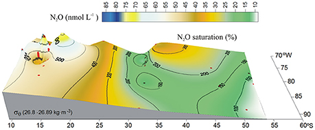
Figure 4. Distribution of N₂O (nmol L⁻¹) along the 26.8 kg m⁻³ isopycnal in the eastern South Pacific. Color code denotes N₂O concentrations. Black contours indicate percentage of gas saturation (%), red dots indicate profile positions.

${\text{NO}}_3^{-}$ distribution displayed a relatively linear increase within the core of AAIW from 60° to 10°S, with a local maximum of 45.6 μmol L⁻¹ at 15°S (Figure 3C); whereas ${\text{NO}}_2^{-}$ distribution was almost constant (< 0.1 μmol L⁻¹) over most of the southern part of the study area (Figure 3D). Similar to N₂O, there was a large increase in ${\text{NO}}_2^{-}$ concentration north of 20°S, with a maximum value of 1.5 μmol L⁻¹ north of 15°S (Figure 3D).

In order to quantify the contribution of AAIW and ESSW within the ESP, we applied the OMP analysis (Tomczak and Large, 1989; Karstensen and Tomczak, 1998). Between 55°and 30°S, the field is dominated by AAIW (>80%, Figure 5A), while further north at about 20°S and where the strongest increase in N₂O was found, both water masses occupied about 50% (Figure 5). Even further north at ~15°S, only about 30% of AAIW remained (Figure 5A). ESSW contribution, by definition, inversely mirrors AAIW (both adding up to 100%, Figure 5B). Making use of the water mass fractions obtained for the meridional transect at ~80°W from the OMP analysis (Figure 6), and the N₂O concentrations in source regions, we calculated the distributions of salinity and N₂O that we expected to find if only mixing were to alter parameter fields. Salinity, being a conservative parameter, serves as a control variable to validate the reconstruction. Reconstructed salinity (Figure 6C) differed only by < 0.03 psu (Figure 6D) from observed salinity (Figure 6B), and supported the validity of estimated mixing. For N₂O, in contrast, we found a difference between “mixing only” (Figure 6F) and the observed field (Figure 6E) of up to 32.5 nmol L⁻¹ (Figure 6G), which can be interpreted as the signature of biogeochemical N₂O cycling.

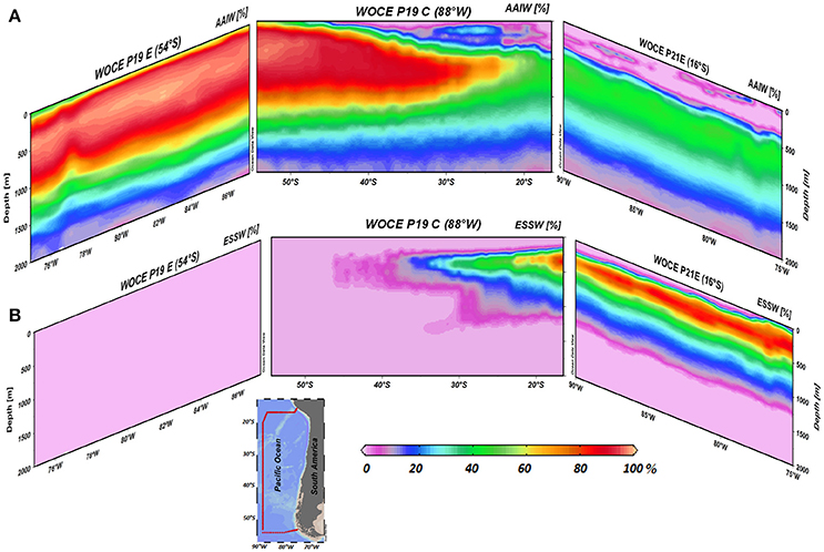
Figure 5. Zonal and meridional distribution of water masses (%) in the eastern South Pacific, (A) AAIW and (B) ESSW. Data include three WOCE transects (P19C, P19E, and P21E). The percentage (fraction of mixing) of AAIW and ESSW in the water column is indicated by the color code (%). The inside figure shows WOCE transect locations.

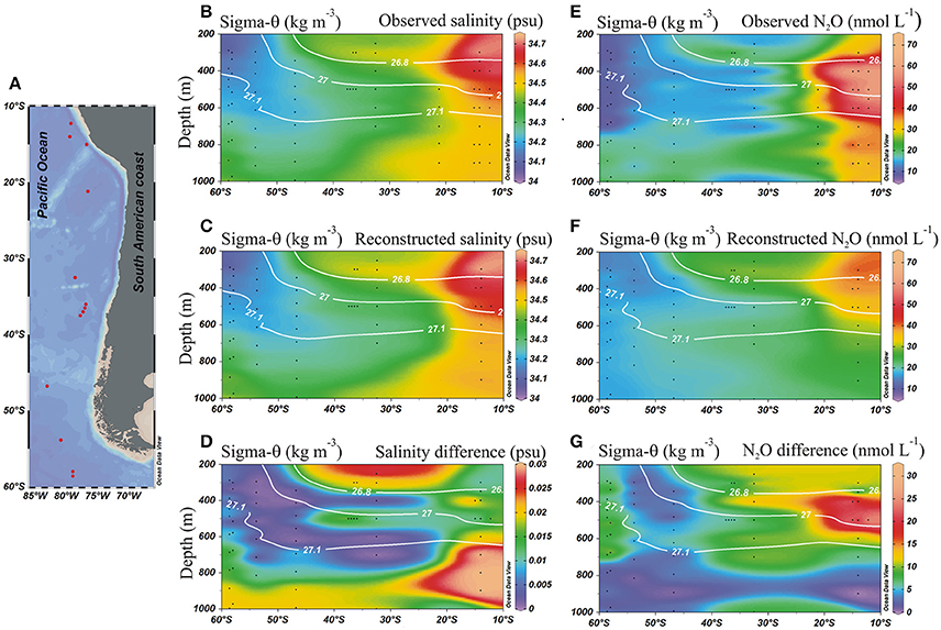
Figure 6. Meridional distribution of salinity and N₂O from observed and reconstructed data in the eastern south Pacific. (A) Stations locations; (B) Observed salinity (psu); (C) Reconstructed salinity from water mass fractions (OMP); (D) Difference between observed and reconstructed salinity distributions; (E) Observed N₂O (nmol L⁻¹); (F) Reconstructed N₂O (nmol L⁻¹) from water mass fractions (OMP); and (G) Difference between observed and reconstructed N₂O (nmol L⁻¹). Black dots indicate sample locations. White lines denote potential density (kg m⁻³).

At mid-latitudes (~20°–30°S), where mixing becomes more important, a change in N₂O distribution is clearly discernable, which is sensitive to the effects of O₂(Figures 2, 3, 5). Combining the age of AAIW with the AOU and N₂O distribution throughout the study area, it was possible to estimate the mean rates of O₂consumption (apparent oxygen utilization rate, AOUR) and N₂O accumulation within the core of AAIW (Table 3). Between 54° and 30°S, we obtained an AOUR of 26.38 nmol L⁻¹ d⁻¹ and a N₂O accumulation rate of 0.61 pmol L⁻¹ d⁻¹; while between 22°S and 18°S, we observed an almost twice as high AOUR and a disproportionately high (~29 times) increase in N₂O accumulation (Table 3). Mixing and biogeochemical cycling operate on different time scales and therefore the dilution of a water mass does not necessarily correlate with its age (i.e., the time spent by the water mass in the inner ocean). The sluggish flow underneath the OMZ generates very long residence times, which in turn may allow for intense N₂O production. CFC derived water ages may not reflect the true age of the water in this region, where significant mixing with the ESSW is present, because a large volume of the original source water may be free of CFC (formed prior to 1950 when CFC was released into the atmosphere), and as such, CFC age cannot represent the age of water masses that contribute to the bulk of the water parcels (Waugh et al., 2003).

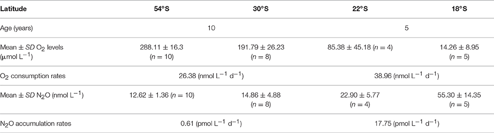
Table 3. Estimated mean rates of O₂ consumption and N₂O accumulation; estimated age and mean O₂ and N₂O levels in two areas: 54°–30°S and 22°–18°S along the AAIW core (27-27.1 kg m⁻³) in the ESP.

Two typical profiles of O₂ and N₂O for north and south of the 20°S (i.e., 16° and 34°S) are shown in Figure 7. These include the OMZ (northern) and ventilated (southern) regions of the ESP. North of 20°S, two N₂O maxima are observed (Figure 7A); one is located in the upper layer (30–80 m depth) and coincides with the sharp upper oxycline, where N₂O production is associated with nitrification and partial denitrification (Farías et al., 2009a; Codispoti, 2010). Another peak is found at greater depths within the lower oxycline, at the boundary between AAIW and ESSW. Despite the formation of a weaker oxycline at this location, enhanced N₂O accumulation continues to be triggered. The layer between these maxima (upper and lower oxycline) is the core of the OMZ, where intense N₂O consumption by denitrification is observed (Farías et al., 2009b) and is mainly composed of ESSW. This double-peak structure is consistent with that found by Kock et al. (2016) in offshore waters of the OMZ off Peru (south of 5°S). In the more oxygenated southern section at 34°S, a typical N₂O profile shows a gradual increase of N₂O with depth (Figure 7B), within the low-O₂ layer, contrasting with profiles from the northern region (Figure 7A).

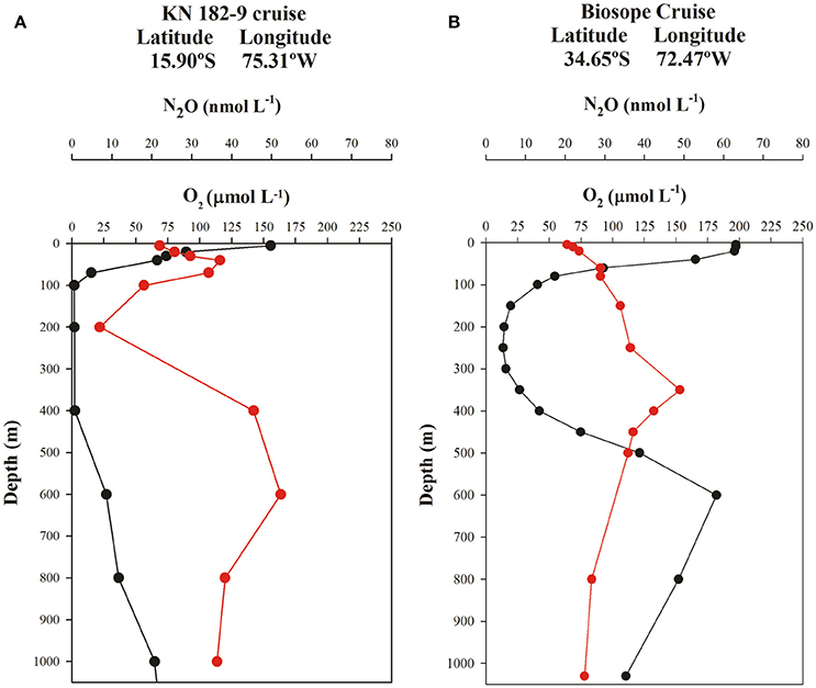
Figure 7. Vertical profiles of O₂ (μmol L⁻¹, black line) and N₂O (nmol L⁻¹, red line) shown at two representative stations (north and south of 20°S) in the eastern South Pacific. (A) OMZ region and (B) ventilated region.

If N₂O is a product of nitrification, the regional correlation of ΔN₂O and AOU, and ΔN₂O and ${\text{NO}}_3^{-}$ (Figure 8), can be used to estimate ΔN₂O associated with a certain level of O₂ consumption caused by the remineralization of POM (Yoshinari, 1976; Nevison et al., 2003). In addition, correlations between ΔN₂O and ${\text{NO}}_2^{-}$ (a good indicator of suboxia/anoxia in OMZs, given that its accumulation is associated with dissimilative ${\text{NO}}_3^{-}$ reduction; Codispoti et al., 1986; Cornejo and Farias, 2012), and between ΔN₂O and N* (indicating the balance between Nitrogen sources and sinks, Gruber and Sarmiento, 1997) suggest the occurrence of denitrification. Between 60° and 20°S, at AAIW core (27–27.1 kg m⁻³), positive correlations were found between ΔN₂O and AOU (Figure 8A, red line), and ΔN₂O and ${\text{NO}}_3^{-}$ (Figure 8B, red line), indicating that N₂O and ${\text{NO}}_3^{-}$ are produced simultaneously to the consumption of O₂ during the northward movement of AAIW, and hence nitrification dominates the nitrogen cycling. We also observed a lack of correlation between ΔN₂O and ${\text{NO}}_2^{-}$ (Figure 8C), and ΔN₂O and N* (Figure 8D), which may indicate that neither in situ denitrification nor signals of denitrification from isopycnal and diapycnal mixing with surrounding water masses are expected. However, between 20° and 10°S, at the same density range, the situation was different. The abrupt increase in ΔN₂O was not accompanied by an AOU increase (Figure 8A). We also observed negative correlations between ΔN₂O and ${\text{NO}}_3^{-}$ (Figure 8B, black dashed line) and ΔN₂O and N* (Figure 8D, black dashed line) and a positive correlation between ΔN₂O and ${\text{NO}}_2^{-}$ (Figure 8C, black dashed line). These trends imply that denitrification produces N₂O (at high AOU/low O₂ concentrations), but also that lateral and vertical mixing may enrich the AAIW core with ${\text{NO}}_3^{-}$ and ${\text{NO}}_2^{-}$ that originates from ESSW (which has relatively high ${\text{NO}}_3^{-}$ and ${\text{NO}}_2^{-}$).

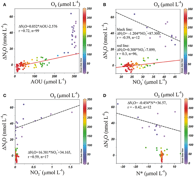
Figure 8. Correlations of (A) ΔN₂O vs. AOU; (B) ΔN₂O vs. ${\text{NO}}_3^{-}$; (C) ΔN₂O vs. ${\text{NO}}_2^{-}$; and (D) ΔN₂O vs. N*, along 27–27.1 kg m⁻³ (AAIW) in the ESP. Color code indicates O₂ concentration. The red line indicates a least-square fit between 60° and 20°S, and the black dashed line is the correlation between 20° and 10°S.

From the ΔN₂O and AOU correlation (Figure 8) it is clear that the low O₂ (25 μmol L⁻¹) and high N₂O (75 nmol L⁻¹; 600 m) concentrations in the core of AAIW at 17.6°S cannot be explained by nitrification only. Moreover, high N₂O concentrations in the ESSW core (26.8 kg m⁻⁻³) at 16°S (76.8 nmol L⁻¹; 350 m) and at 13.3°S (87 nmol L⁻¹; 400 m) are observed and interpreted as a clear sign for denitrifying processes. The OMP analysis (Figure 5) revealed mixing between AAIW, a water mass from the south dominated by nitrification, and ESSW, a water mass under the impact of denitrification processes from the north, in the transition area underneath the OMZ. As such it is primarily the mixing that creates high N₂O-values, even in the core of the AAIW.

Studies have shown that significant quantities of N₂O are produced by Bacteria and Archaea at O₂ concentrations below 5 μmol L⁻¹ (Frame and Casciotti, 2010; Santoro et al., 2011; Löscher et al., 2012). On the other hand, Kalvelage et al. (2011) found that aerobic and anaerobic N-cycling pathways in the OMZ can co-occur over a larger range of O₂ concentrations than previously thought. They have found that anammox, which is the anaerobic oxidation of ammonium resulting in the production of dinitrogen gas and nitrogen loss, could take place under O₂ levels up to about 20 μmol L⁻¹, while anaerobic ${\text{NO}}_3^{-}$ reduction was fully active up to at least 25 μmol L⁻¹. Thus, apparently 25 μmol L⁻¹ of O₂ is very close to where both aerobic and anaerobic processes can occur simultaneously. Hence, part of the signal may point toward anammox processes in the lower part of the OMZ, impacting the AAIW density range.

Another possible explanation for the increase in N₂O north of 20°S is the higher bacterial activity product of the increase in primary productivity (PP) and the subsequent export of POM to the studied depth range (Suess, 1980). We have no direct estimates of PP during sampling, but considering the climatological distribution of surface chlorophyll from satellite data (Thomas et al., 2001; Yuras et al., 2005), no enhanced PP is found between 20° and 10°S, and none in comparison with the region further south (Farías et al., 2009b; Fernandez et al., 2009; Aracena et al., 2011). The most widespread and biologically productive areas are found over the continental shelf between 42°–50°S, 32°–37°S, and 0°–10°S (Kellog and Mohriak, 2001). As such, we exclude regionally enhanced POM export as a cause of the N₂O increase between 20° and 10°S.

It has been shown that changes in the ventilation rates of AAIW have immediate consequences on the oceanic inventories of O₂ and N-species (Galbraith et al., 2004; Meissner et al., 2005). Under reported scenarios of reduced AAIW formation (Downes et al., 2009), the AAIW O₂ inventory will also decrease and, according to our data, this would result in an increase in the N₂O inventory. In a previous study using an oceanic biogeochemical model to predict the impact of climate change on O₂ cycling, Matear et al. (2000) found a potential O₂ reduction of up to 70 μmol L⁻¹ in the Southern Ocean. In general, ocean models predict a global decline in the O₂ inventory of up to 7% over the next century, and this scenario will continue for at least a thousand years into the future (Keeling et al., 2010). Variability in intermediate water masses is tightly linked to global changes given their relatively close connection to the surface ocean (Banks et al., 2000; Matear et al., 2000). Based on our observations, we expect that a decrease in O₂ in source waters will result in an even larger accumulation of N₂O between ESSW and AAIW.

Conclusion and Implications

This study reports N₂O accumulation in intermediate waters, with a focus on Antarctic Intermediate Water (AAIW, 27–27.1 kg m⁻³) in the eastern South Pacific Ocean. Here, we found two distinct N₂O cycling regimes: first, a regime of slow accumulation of N₂O in waters that are well-oxygenated and located between 20° and 60°S. ΔN₂O to AOU correlation suggest that this accumulation is the result of nitrification. The second regime is of an abrupt increase in N₂O north of 20°S. Different correlations suggest that either nitrification (in low O₂ waters) or denitrification may be responsible for the observed increase.

A water mass mixing analysis was used to investigate the ΔN₂O with respect to the dominant water masses: the high-O₂ AAIW that originates in the south; and the low-O₂ ESSW that originates at the equator. Notably, the N₂O maximum found at the core of AAIW was associated with water relatively oxygenated (O₂ concentration of25 μmol L⁻¹). Our findings did not support the association between increased productivity/organic matter supply in this region and high N₂O accumulation. We conclude that the sluggish flow of water in the region underneath the OMZ, and the subsequent extended residence times water masses, facilitate intense N₂O production. Therefore, N₂O production at intermediate water depths should not be disregarded in ocean N₂O budgets.

Author Contributions

All authors contributed extensively to the work presented in this paper: CC analyzed data and wrote the manuscript. JK supervised OMP analysis and edited the manuscript. LF supervised the project, and edited the manuscript. All authors discussed the results and commented on the manuscript at all stages.

Conflict of Interest Statement

The authors declare that the research was conducted in the absence of any commercial or financial relationships that could be construed as a potential conflict of interest.

Acknowledgments

The first author wishes to acknowledge the Instituto Antartico Chileno (INACH) for the grant received from the Graduate Thesis Support Program (Project M_07-10) and also wishes to thank the German Academic Exchange Service (DAAD) for the research grant received (scholarships of short duration). JK acknowledges funding from the German Science Foundation as part of the Sonderforschungsbereich 754 Climate-Biogeochemistry Interactions in the Tropical Ocean. This research is a contribution by the FONDAP (grant 1501007 and 1511009) program. Additionally, LF was supported by ICM 120019 project (IMO). All authors thank Drs. Hermann W. Bange and Annette Kock who kindly provided N₂O data from cruise M77-4 (SFB 754). We thank Lynne D. Talley for the invitation to participate in the SAMFLOC cruise and we appreciate the comments and corrections done by Dr. Caitlin Frame to the final version of this manuscript.

References

Anderson, L. A., and Sarmiento, J. L. (1994). Redfield ratios of remineralization determined by nutrient data analysis. Glob. Biogeochem. Cycle 8, 65–80 doi: 10.1029/93GB03318
Aracena, C., Lange, C., Iriarte, J. L., Rebolledo, L., and Pantoja, S. (2011). Latitudinal patterns of export production recorded in surface sediments of the Chilean Patagonian fjords (41°–55°S) as a response to water column productivity. Cont. Shelf Res. 31, 340–355. doi: 10.1016/j.csr.2010.08.008
Bange, H. W. (2008). “Gaseous nitrogen compounds (NO, N2O, N2, NH3) in the ocean,” in Nitrogen in the Marine Environment, eds D. Capone, D. Bronk, M. Mulholland, and E. Carpenter (Amsterdam: Elsevier), 51–93.
Bange, H. W., and Andreae, M. O. (1999). Nitrous oxide in the deep waters of the world's oceans. Glob. Biogeochem. Cycle 13, 1127–1135. doi: 10.1029/1999GB900082
Bange, H. W., Naqvi, S. W. A., and Codispoti, L. A. (2005). The nitrogen cycle in the Arabian Sea. Prog. Oceanogr. 65, 145–158. doi: 10.1016/j.pocean.2005.03.002
Banks, H. T., Wood, R. A., Gregory, J. M., Johns, T. C., and Jones, G. S. (2000). Are observed decadal changes in intermediate water masses a signature of anthropogenic climate change?. Geophys. Res. Lett. 27, 2961–2964. doi: 10.1029/2000GL011601
Broecker, W. S., Andree, M., Bonani, G., Wolfli, W., Oeschger, H., Klas, M., et al. (1988). Preliminary estimates for the radiocarbon age of deep water in the glacial ocean. Paleoceanography 3, 659–669.
Canfield, D. E., Stewart, F. J., Thamdrup, B., De Brabandere, L., Dalsgaard, T., DeLong, E. F., et al. (2010). A cryptic sulfur cycle in oxygen-minimum zone waters off the Chilean coast. Science 330, 1375–1378. doi: 10.1126/science.1196889
Codispoti, L. A. (2010). Interesting times for marine N2O. Science 237, 1339–1340 doi: 10.1126/science.1184945
Codispoti, L. A., Brandes, J. A., Christensen, J. P., Devol, A. H., Naqvi, S. W. A., Paerl, H. S., et al. (2001). The oceanic fixed nitrogen and nitrous oxide budgets: moving targets as we enter the anthropocene? Sci. Mar. 65, 85–105. doi: 10.3989/scimar.2001.65s285
Codispoti, L. A., Friederich, G. E., Packard, T. T., Glover, H. E., Kelly, P. J., Spinrad, R. W., et al. (1986). High nitrite levels off northern Peru: a signal of instability in the marine denitrification rate. Science 233, 1200–1202. doi: 10.1126/science.233.4769.1200
Cornejo, M., and Farias, L. (2012). Following the N2O consumption in the oxygen minimum zone of the eastern South Pacific. Biogeosciences 9, 3205–3212. doi: 10.5194/bg-9-3205-2012
Dalsgaard, T., Stewart, F. J., Thamdrup, B., De Brabandere, L., Revsbech, N. P., Ulloa, O., et al. (2014). Oxygen at nanomolar levels reversibly suppresses process rates and gene expression in anammox and denitrification in the oxygen minimum zone off Northern Chile. MBio 5, e01966–e01914. doi: 10.1128/mBio.01966-14
De Pol-Holz, R., Ulloa, O., Lamy, F., Dezileau, L., Sabatier, P., and Hebbeln, D. (2007). Late quaternary variability of sedimentary nitrogen isotopes in the eastern South Pacific Ocean. Paleoceanography 22, PA2207. doi: 10.1029/2006pa001308
Downes, S. M., Bindoff, N. L., and Rintoul, S. R. (2009). Impacts of climate change on the subduction of mode and intermediate water masses in the Southern Ocean. J. Clim. 22, 3289–3302. doi: 10.1175/2008JCLI2653.1
Farías, L., Castro-Gonzalez, M., Cornejo, M., Charpentier, J., Faundez, J., Boontanon, N., et al. (2009a). Denitrification and nitrous oxide cycling within the upper oxycline of the oxygen minimum zone off the eastern tropical South Pacific. Limnol. Oceanogr. 54, 132–144. doi: 10.4319/lo.2009.54.1.0132
Farías, L., Fernández, C., Faúndez, J., Cornejo, M., and Alcaman, M. E. (2009b). Chemolithoautotrophic production mediating the cycling of the greenhouses gases N2O and CH4 in an upwelling ecosystem. Biogeosciences 6, 3053–3069. doi: 10.5194/bg-6-3053-2009
Fernandez, C., Farías, L., and Alcamam, M. E. (2009). Primary production and nitrogen regeneration processes in surface waters of the Peruvian upwelling system. Prog. Oceanogr. 83, 159–168. doi: 10.1016/j.pocean.2009.07.010
Fiedler, P. C., and Talley, L. D. (2006). Hydrography of the eastern tropical Pacific: a review. Prog. Oceanogr. 69, 143–180. doi: 10.1016/j.pocean.2006.03.008
Frame, C. H., and Casciotti, K. L. (2010). Biogeochemical controls and isotopic signatures of nitrous oxide production by a marine ammonia-oxidizing bacterium. Biogeosciences 7, 2695–2709. doi: 10.5194/bg-7-2695-2010
Freing, A., Wallace, D. W. R., and Bange, H. W. (2012). Global oceanic production of nitrous oxide. Phil. Trans. R. Soc. B 367, 1254–1255. doi: 10.1098/rstb.2011.0360
Freing, A., Wallace, D. W. R., Tanhua, T., Walter, S., and Bange, H. W. (2009). North Atlantic production of nitrous oxide in the context of changing atmospheric levels. Glob. Biogeochem. Cycle. 23, GB4015. doi: 10.1029/2009GB003472
Fujii, A., Toyoda, S., Yoshida, O., Watanabe, S., Sasaki, K., and Yoshida, N. (2013). Distribution of nitrous oxide dissolved in water masses in the eastern subtropical North Pacific and its origin inferred from isotopomer analysis. J. Oceanogr. 69, 147–157. doi: 10.1007/s10872-012-0162-4
Galbraith, E. D., Kienast, M., Pedersen, T. F., and Calvert, S. E. (2004). Glacial-interglacial modulation of the marine nitrogen cycle by high-latitude O2 supply to the global thermocline. Paleoceanography 19, PA4007. doi: 10.1029/2003PA001000
Garcia, H. E., and Gordon, L. I. (1992). Oxygen solubility in seawater: better fitting equations. Limnol. Oceanogr. 37, 1307–1312. doi: 10.4319/lo.1992.37.6.1307
Georgi, D. (1979). Modal properties of Antarctic intermediate water in the Southeast Pacific and the South Atlantic. J. Phys. Oceanogr. 9, 456–468. doi: 10.1175/1520-0485(1979)009<0456:MPOAIW>2.0.CO;2
Goreau, T. J., Kaplan, W. A., Wofsy, S. C., McElroy, M. B., Valois, F. W., and Watson, S. W. (1980). Production of NO2- and N2O by nitrifying bacteria at reduced concentrations of oxygen. Appl. Environ. Microbiol. 40, 526–532.
Gruber, N., and Sarmiento, J. L. (1997). Global patterns of marine nitrogen fixation and denitrification. Glob. Biogeochem. Cycle 11, 235–266. doi: 10.1029/97GB00077
Hupe, A., and Kartsensen, J. (2000). Redfield stoichiometry in Arabian Sea subsurface waters. Global Biogeochem. Cycle 14, 357–372. doi: 10.1029/1999GB900077
Kalvelage, T., Jensen, M. M., Contreras, S., Revsbech, N. P., Lam, P., Günter, M., et al. (2011). Oxygen sensitivity of anammox and coupled N-Cycle processes in oxygen minimum zones. PLoS ONE 6:e29299. doi: 10.1371/journal.pone.0029299
Karstensen, J., Stramma, L., and Visbeck, M. (2008). Oxygen minimum zones in the eastern tropical Atlantic and Pacific oceans. Prog. Oceanogr. 77, 331–350. doi: 10.1016/j.pocean.2007.05.009
Karstensen, J., and Tomczak, M. (1998). Age determination of mixed water masses using CFC and oxygen data. J. Geophys. Res. 103, 18599. doi: 10.1029/98jc00889
Keeling, R. F., Körtzinger, A., and Gruber, N. (2010). Ocean deoxygenation in a warming world. Annu. Rev. Mar. Sci. 2, 199–229. doi: 10.1146/annurev.marine.010908.163855
Kellog, J., and Mohriak, W. U. (2001). “The tectonic and geological environment of coastal South America,” in Coastal Marine Ecosystems of Latin America, eds U. Seeliger and B. Kjerfve (Berlin; Heidelberg; Springer-Verlag), 2–16.
Kessler, W. S. (2006). The circulation of the eastern tropical Pacific: a review. Prog. Oceanogr. 69, 181–217. doi: 10.1016/j.pocean.2006.03.009
Kock, A., Arévalo-Martínez, D. L., Löscher, C. R., and Bange, H. W. (2016). Extreme N2O accumulation in the coastal oxygen minimum zone off Peru. Biogeosciences 13, 827–840. doi: 10.5194/bg-13-827-2016
Llanillo, P. J., Karstensen, J., Pelegrí, J. L., and Stramma, L. (2013). Physical and biogeochemical forcing of oxygen and nitrate changes during El Ni-o/El Viejo and La Ni-a/La Vieja upper-ocean phases in the tropical eastern South Pacific along 86°W. Biogeosciences 10, 6339–6355. doi: 10.5194/bg-10-6339-2013
Löscher, C. R., Kock, A., Könneke, M., LaRoche, J., Bange, H. W., and Schmitz, R. A. (2012). Production of oceanic nitrous oxide by ammonia-oxidizing archaea. Biogeosciences 9, 2419–2429. doi: 10.5194/bg-9-2419-2012
Machida, T., Nakazawa, T., Fujii, Y., Aoki, S., and Watanabe, O. (1995). Increase in the atmospheric nitrous oxide concentration during the last 250 years. Geophys. Res. Lett. 22, 2921–2924. doi: 10.1029/95GL02822
Matear, R. J., Hirst, A. C., and McNeil, B. I. (2000). Changes in dissolved oxygen in the Southern Ocean with climate change. Geochem. Geophys. Geosyst. 1:2000GC000086. doi: 10.1029/2000GC000086
McCartney, M. S. (1977). “Subantarctic mode water,” in A Voyage of Discovery: George Deacon 70th Anniversary Volume, ed M. Angel (Oxford: Pergamon Press), 103–119.
Meissner, K. J., Galbraith, E. D., and Völker, C. (2005). Denitrification under glacial and interglacial conditions: a physical approach. Paleoceanography 20, PA3001. doi: 10.1029/2004PA001083
Naqvi, S. W. A., and Noronha, R. J. (1991). Nitrous oxide in the Arabian Sea. Deep Sea Res. 38, 871–890. doi: 10.1016/0198-0149(91)90023-9
Nevison, C. D., Butler, J. H., and Elkins, J. W. (2003). Global distribution of N2O and the ΔN2O-AOU yield in the subsurface ocean. Glob. Biogeochem. Cycle 17, 1119 doi: 10.1029/2003GB002068
Nevison, C. D., Lueker, T. J., and Weiss, R. F. (2004). Quantifying the nitrous oxide source from coastal upwelling. Glob. Biogeochem. Cycle 18, GB1018. doi: 10.1029/2003GB002110
Nevison, C. D., Weiss, R. F., and Erickson III, D. J. (1995). Global oceanic nitrous oxide emissions. J. Geophys. Res. 100, 15809–15820. doi: 10.1029/95jc00684
Poth, M., and Focht, D. D. (1985). 15N Kinetic analysis of N2O production by nitrosomonas europaea: an examination of nitrifier denitrification. Appl. Environ. Microbiol. 49, 1134–1141.
Revsbech, N. P., Larsen, L. H., Gundersen, J., Dalsgaard, T., Ulloa, O., and Thamdrup, B. O. (2009). Determination of ultra-low oxygen concentrations in oxygen minimum zones by the STOX sensor. Limnol. Oceanogr. Methods 7, 371–381. doi: 10.4319/lom.2009.7.371
Santoro, A. E., Buchwald, C., McIlvin, M. R., and Casciotti, K. L. (2011). Isotopic signature of N2O produced by marine ammonia-oxidizing Archaea. Science 333, 1282–1285. doi: 10.1126/science.1208239
Schneider, B., Karstensen, J., Oschlies, A., and Schlitzer, R. (2005). Model-based evaluation of methods to determine C:N and N:P regeneration ratios from dissolved nutrients. Glob. Biogeochem. Cycle 19, GB2009. doi: 10.1029/2004GB002256
Silva, N., Rojas, N., and Fedele, A. (2009). Water masses in the humboldt current system: properties, distribution, and the nitrate deficit as a chemical water mass tracer for equatorial subsurface water off Chile. Deep Sea Res. II 56, 1004–1020. doi: 10.1016/j.dsr2.2008.12.013
Suess, E. (1980). Particulate organic carbon flux in the oceans: surface and oxygen utilization. Nature 288, 260–271. doi: 10.1038/288260a0
Suntharalingam, P., and Sarmiento, J. L. (2000). Factors governing the oceanic nitrous oxide distribution: simulations with an ocean general circulation model. Glob. Biogeochem. Cycle 14, 429–454. doi: 10.1029/1999GB900032
Sverdrup, H. U., Johnson, M. W., and Fleming, R. H. (1942). The Oceans: Their Physics, Chemistry, and General Biology. New York, NY: Prentice Hall.
Talley, L. (1999). “Some aspects of ocean heat transport by the shallow, intermediate and deep overturning circulation,” in Mechanisms of Global Climate Change at Millenial Time Scales, eds P. Clark, R. Webb, and L. Keigwin (Washington, DC: Geophysical Monograph Series), 1–22.
Thomas, A. C., Carr, M.-E., and Strub, P. T. (2001). Chlorophyll variability in eastern boundary currents. Geophys. Res. Lett. 28, 3421–3424. doi: 10.1029/2001GL013368
Tomczak, M., and Large, D. G. B (1989). Optimum multiparameter analysis of mixing in the thermocline of the eastern Indian Ocean. J. Geophys. Res. 94, 16141–16149. doi: 10.1029/JC094iC11p16141
Tsuchiya, M., and Talley, L. D. (1996). Water-property distributions along an eastern Pacific hydrographic section at 135W. J. Mar. Res. 54, 541–564. doi: 10.1357/0022240963213583
Walker, S. J., Weiss, R. F., and Salameh, P. K. (2000). Reconstructed histories of the annual mean atmospheric mole fractions for the halocarbons CFC-11 CFC-12, CFC-113, and carbon tetrachloride. J. Geophys. Res. 105, 14285–14296. doi: 10.1029/1999jc900273
Warner, M. J., and Weiss, R. F. (1985). Solubilities of chlorofluorocarbons 11 and 12 in water and seawater. Deep Sea Res. 32, 1485–1497. doi: 10.1016/0198-0149(85)90099-8
Waugh, D. W., Hall, T. M., and Haine, T. W. N. (2003). Relation- ships among tracer ages. J. Geophys. Res. 108, 3138. doi: 10.1029/2002JC001325
Weiss, R., and Price, B. A. (1980). Nitrous oxide solubility in water and seawater. Mar. Chem. 8, 347–359. doi: 10.1016/0304-4203(80)90024-9
Wyrtki, K. (1963). The Horizontal and Vertical Field of Motion in the Peru Current, Vol. 8, Bulletin of the Scripps Institution of Oceanography. Berkeley, CA: University of California Press.
Wyrtki, K. (1967). Circulation and water masses in the eastern equatorial Pacific Ocean. Int. J. Oceanol. Limol. 1, 117–147.
Yamagishi, H., Westley, M. B., Popp, B. N., Toyoda, S., Yoshida, N., Watanabe, S., et al. (2007). Role of nitrification and denitrification on the nitrous oxide cycle in the eastern tropical North Pacific and Gulf of California. J. Geophys. Res. 112, G02015. doi: 10.1029/2006jg000227
Yoshinari, T. (1976). Nitrous oxide in the sea. Mar. Chem. 4, 189–202. doi: 10.1016/0304-4203(76)90007-4
Keywords: N2O accumulation, nitrification, denitrification, eastern South Pacific Ocean, water mass analysis, intermediate waters
Citation: Carrasco C, Karstensen J and Farias L (2017) On the Nitrous Oxide Accumulation in Intermediate Waters of the Eastern South Pacific Ocean. Front. Mar. Sci. 4:24. doi: 10.3389/fmars.2017.00024
Received: 24 July 2016; Accepted: 20 January 2017;
Published: 03 February 2017.
Edited by:
Carol Robinson, University of East Anglia, UKReviewed by:
Andrew Paul Rees, Plymouth Marine Laboratory, UKRavi Bhushan, Physical Research Laboratory, India
Copyright © 2017 Carrasco, Karstensen and Farias. This is an open-access article distributed under the terms of the Creative Commons Attribution License (CC BY). The use, distribution or reproduction in other forums is permitted, provided the original author(s) or licensor are credited and that the original publication in this journal is cited, in accordance with accepted academic practice. No use, distribution or reproduction is permitted which does not comply with these terms.
*Correspondence: Laura Farías, laura.farias@udec.cl