Assessing Spatiotemporal Variations of Landsat Land Surface Temperature and Multispectral Indices in the Arctic Mackenzie Delta Region between 1985 and 2018

 ,
,
Abstract
:
1. Introduction
2. Materials and Methods
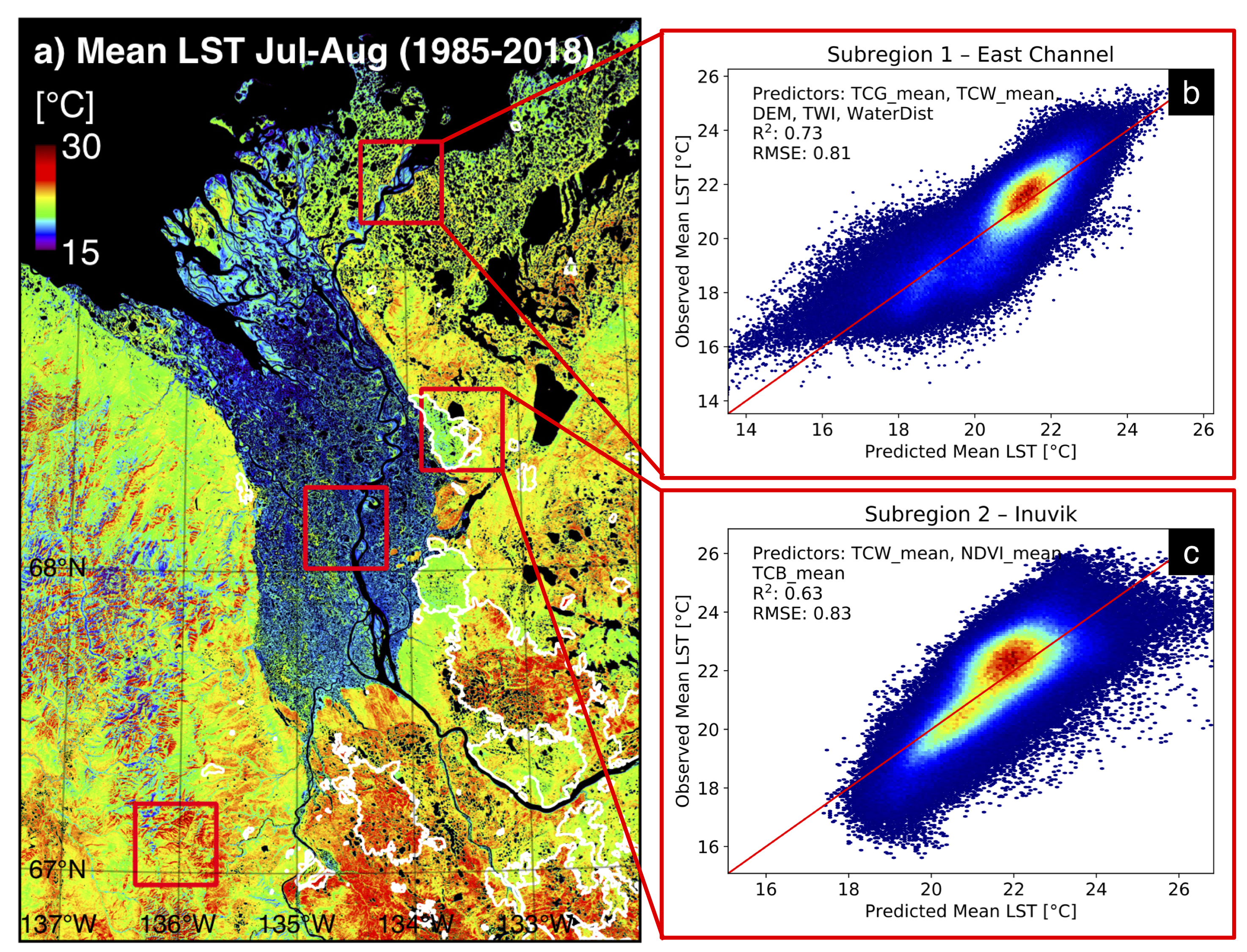
2.1. Study Area
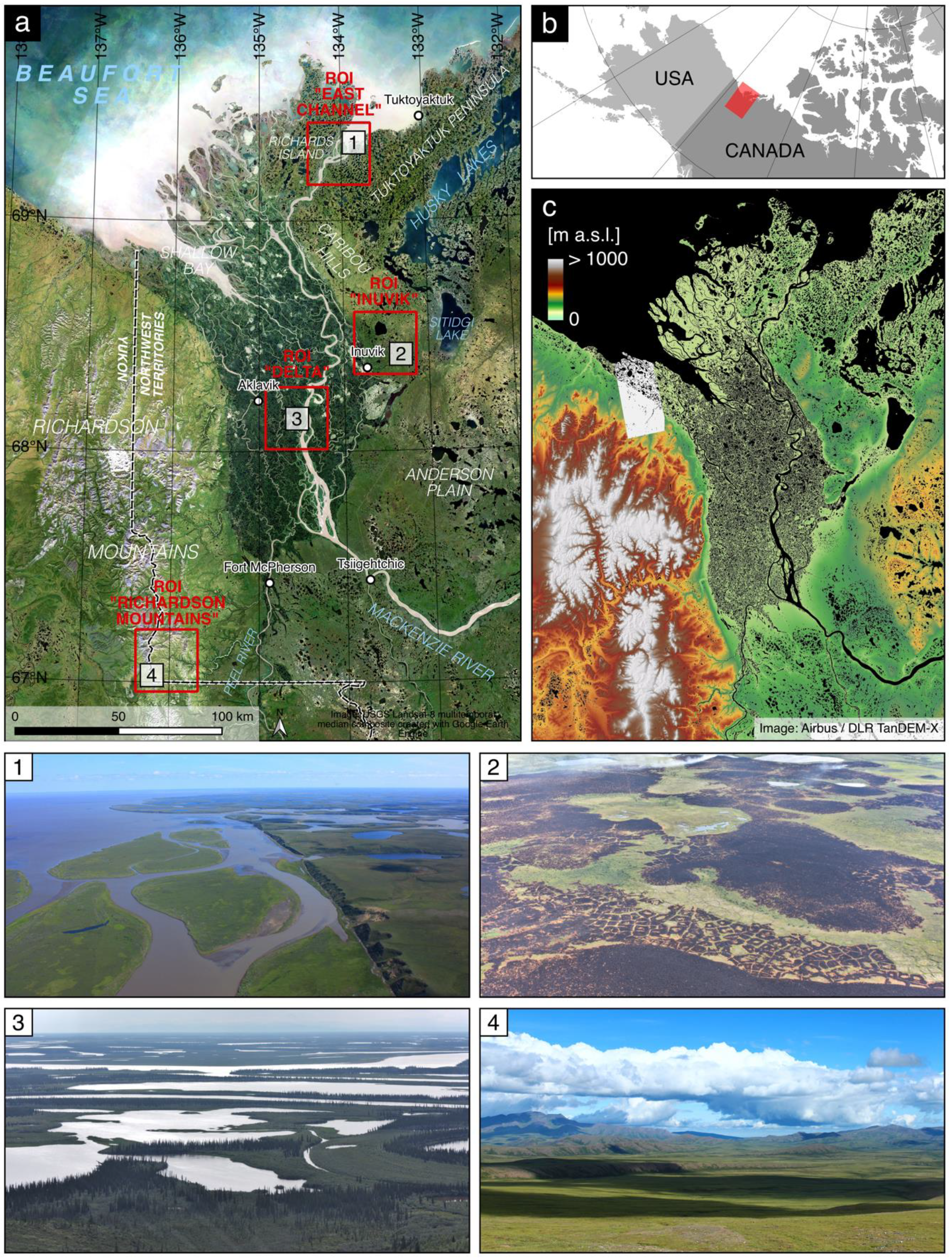
2.2. Data
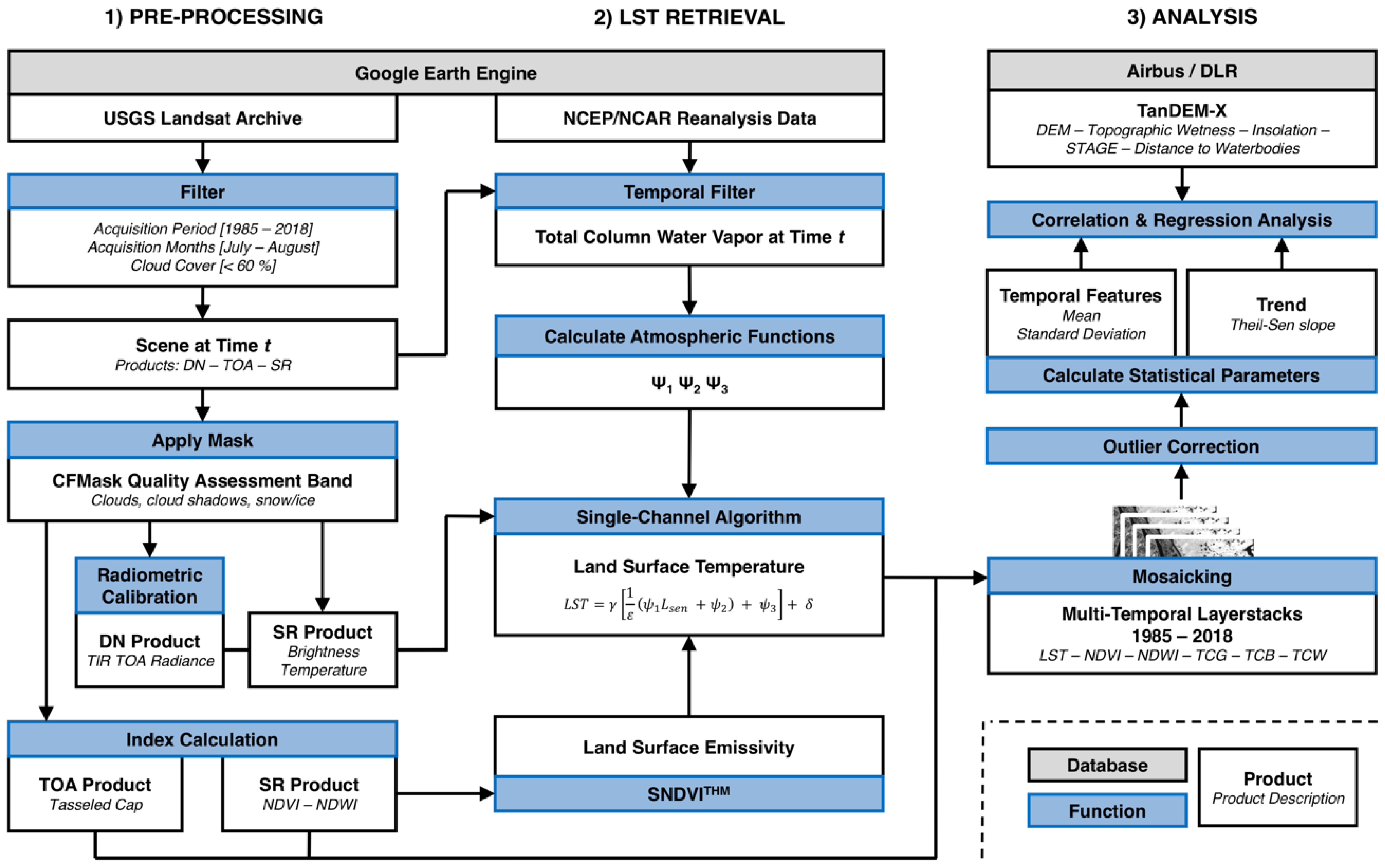
2.3. Methods
2.3.1. Pre-Processing and Retrieval of Multispectral Indices
2.3.2. Retrieval of Land Surface Temperature
2.3.3. Statistical Analysis
3. Results
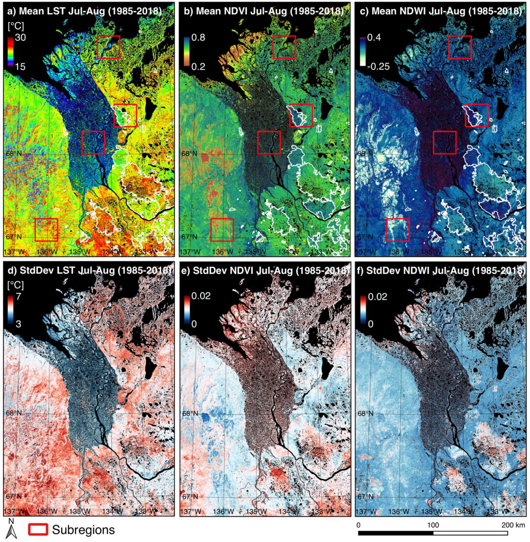
3.1. Mean Summer Land Surface Temperature, NDVI, and NDWI
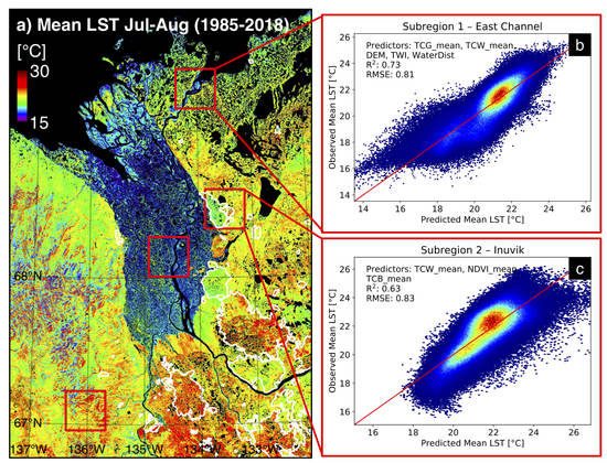
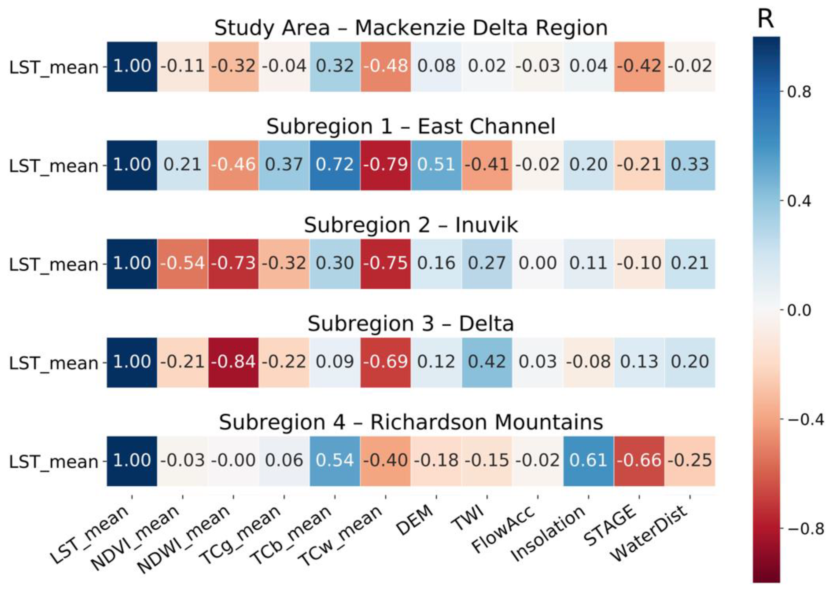
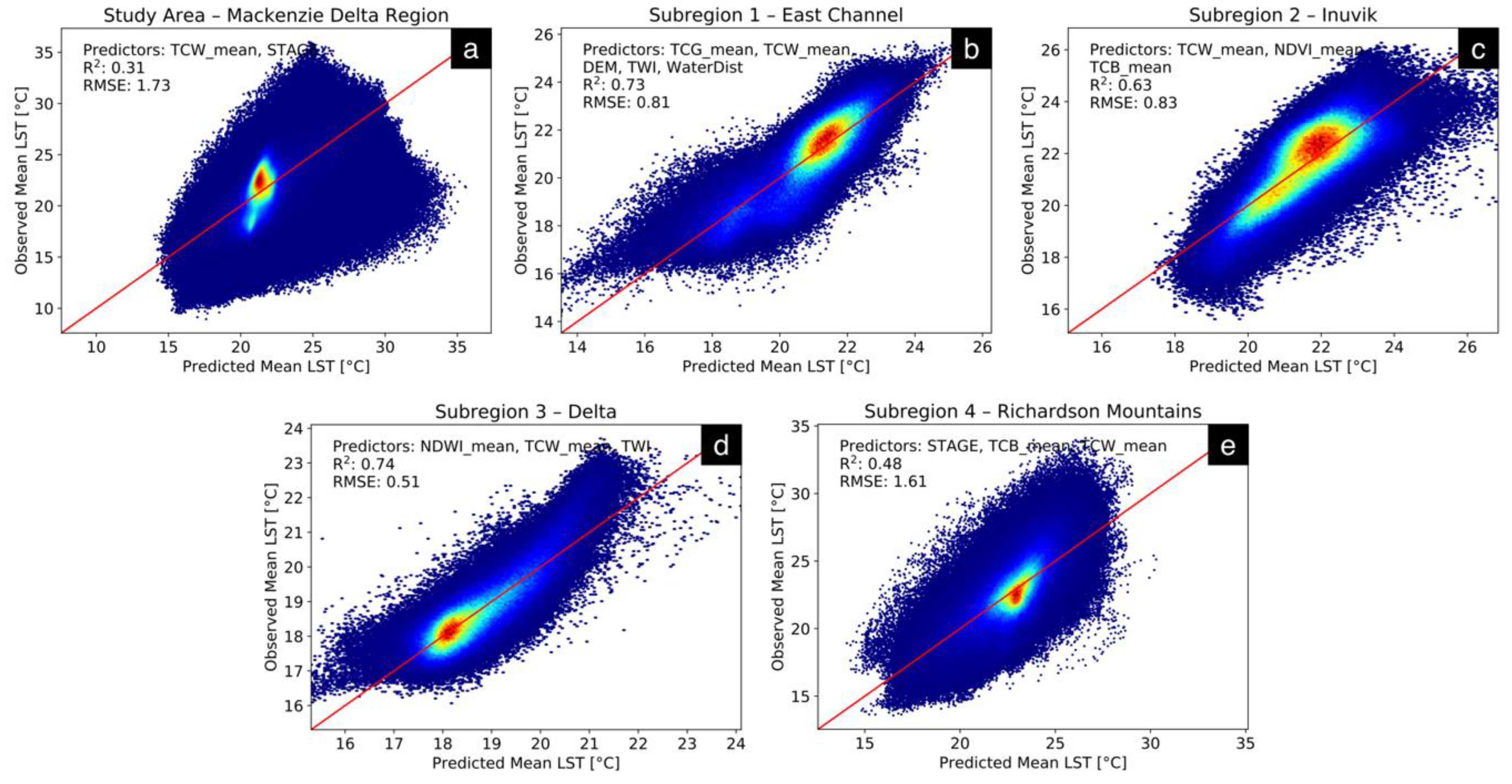
3.2. Correlation and Regression between LST and Environmental Factors
3.3. Temporal Dynamics of LST, NDVI, and NDWI
3.4. Local Temporal Dynamics of LST, NDVI, and NDWI
4. Discussion
4.1. Processing of LST Using Dense Landsat Time Series
4.2. Relation of LST to Other Environmental Variables in the Mackenzie Delta Region
4.3. Temporal Changes
5. Conclusions
Author Contributions
Funding
Acknowledgments
Conflicts of Interest
Appendix A

Appendix B
| Feature | Description | Year/Period | Source |
|---|---|---|---|
| LST_mean | Mean of Land Surface Temperature | 1985−2018 | Landsat |
| LST_stdDev | Standard Deviation of Land Surface Temperature | 1985−2018 | Landsat |
| LST_ts | Theil-Sen trend of Summer Land Surface Temperature | 1985−2018 | Landsat |
| TCg_mean | Mean of Tasseled Cap Greenness | 1985−2018 | Landsat |
| TCg_stdDev | Standard Deviation of Tasseled Cap Greenness | 1985−2018 | Landsat |
| TCg_ts | Theil-Sen trend of Tasseled Cap Greenness | 1985−2018 | Landsat |
| TCb_mean | Mean of Tasseled Cap Brightness | 1985−2018 | Landsat |
| TCb_stdDev | Standard Deviation of Tasseled Cap Brightness | 1985−2018 | Landsat |
| TCb_ts | Theil-Sen trend of Tasseled Cap Brightness | 1985−2018 | Landsat |
| TCw_mean | Mean of Tasseled Cap Wetness | 1985−2018 | Landsat |
| TCw_stdDev | Standard Deviation of Tasseled Cap Wetness | 1985−2018 | Landsat |
| TCw_ts | Theil-Sen trend of Tasseled Cap Wetness | 1985−2018 | Landsat |
| NDVI_mean | Mean of NDVI | 1985−2018 | Landsat |
| NDVI_stdDev | Standard Deviation of NDVI | 1985−2018 | Landsat |
| NDVI_ts | Theil-Sen trend of NDVI | 1985−2018 | Landsat |
| NDWI_mean | Mean of NDWI | 1985−2018 | Landsat |
| NDWI_stdDev | Standard Deviation of NDWI | 1985−2018 | Landsat |
| NDWI_ts | Theil-Sen trend of NDWI | 1985−2018 | Landsat |
| DEM | Terrain Elevation | 2011−2012 | TanDEM-X |
| TWI | Topographic Wetness Index | 2011−2012 | TanDEM-X |
| FlowAcc | Flow Accumulation of Multi-Flow-Direction Approach | 2011−2012 | TanDEM-X |
| Insolation | Potential Annual Solar Insolation | 2011−2012 | TanDEM-X |
| STAGE | Terrain Exposition // Northness // Transformed Aspect | 2011−2012 | TanDEM-X |
| WaterDist | Euclidean Distance to Waterbody | – | Vector Data |
Appendix C
| Study Area–Mackenzie Delta Region (Figure 6a) | R2: 0.307 | RMSE: 1.730 | BIC: 2.351e+08 | |||||
|---|---|---|---|---|---|---|---|---|
| coef | z-score coef | std err | t | P>|t| | [0.025 | 0.975] | VIF | |
| Intercept | 19.6059 | −2.234e−10 | 0.001 | 3.23e+04 | 0.000 | 19.605 | 19.607 | – |
| TCW_mean | −23.4571 | −0.3914 | 0.007 | −3351.713 | 0.000 | −23.471 | −23.443 | 1.175 |
| STAGE | −41.6145 | −0.2687 | 0.004 | −2301.084 | 0.000 | −9.071 | −9.056 | 1.175 |
| Subregion 1–East Channel (Figure 6b) | R2: 0.726 | RMSE: 0.814 | BIC: 1.464e+06 | |||||
|---|---|---|---|---|---|---|---|---|
| coef | z-score coef | std err | t | P>|t| | [0.025 | 0.975] | VIF | |
| Intercept | 17.5934 | −7.582e−08 | 0.008 | 2251.605 | 0.000 | 17.578 | 17.609 | – |
| TCG_mean | 3.7484 | 0.0641 | 0.045 | 83.662 | 0.000 | 3.661 | 3.836 | 1.294 |
| TCW_mean | −41.8219 | −0.650 | 0.048 | −869.013 | 0.000 | −41.916 | −41.728 | 1.233 |
| DEM | 0.0086 | 0.0784 | 0.000 | 78.754 | 0.000 | 0.008 | 0.009 | 2.179 |
| TWI | −0.1850 | −0.2242 | 0.001 | −229.099 | 0.000 | −0.187 | −0.183 | 2.107 |
| WaterDist | 0.0019 | 0.1787 | 7.77e−06 | 243.961 | 0.000 | 0.002 | 0.002 | 1.180 |
| Subregion 2–Inuvik (Figure 6c) | R2: 0.629 | RMSE: 0.834 | BIC: 2.069e+06 | |||||
|---|---|---|---|---|---|---|---|---|
| coef | z-score coef | std err | t | P>|t| | [0.025 | 0.975] | VIF | |
| Intercept | 21.5127 | −2.584e−15 | 0.013 | 1693.969 | 0.000 | 21.488 | 21.538 | – |
| TCW_mean | −52.6900 | −0.6855 | 0.080 | −660.302 | 0.000 | −52.84 | −52.534 | 2.426 |
| NDVI_mean | −4.5934 | −0.2387 | 0.017 | −277.957 | 0.000 | −4.626 | −4.561 | 1.659 |
| TCB_mean | −2.6552 | −0.0571 | 0.044 | −60.300 | 0.000 | −2.741 | −2.569 | 2.020 |
| Subregion 3–Delta (Figure 6d) | R2: 0.743 | RMSE: 0.511 | BIC: 7.426e+05 | |||||
|---|---|---|---|---|---|---|---|---|
| coef | z-score coef | std err | t | P>|t| | [0.025 | 0.975] | VIF | |
| Intercept | 20.4862 | 6.883e−08 | 0.007 | 3084.968 | 0.000 | 20.473 | 20.499 | – |
| NDWI_mean | −10.3214 | −0.6846 | 0.015 | −690.675 | 0.000 | −10.351 | −10.292 | 1.894 |
| TCW_mean | −9.1922 | −0.1687 | 0.058 | −159.725 | 0.000 | −9.305 | −9.079 | 2.151 |
| TWI | 0.0868 | 0.1208 | 0.001 | 148.972 | 0.000 | 0.086 | 0.088 | 1.268 |
| Subregion 4–Richardson Mountains (Figure 6e) | R2: 0.479 | RMSE: 1.614 | BIC: 3.785e+06 | |||||
|---|---|---|---|---|---|---|---|---|
| coef | z-score coef | std err | t | P>|t| | [0.025 | 0.975] | VIF | |
| Intercept | 18.5392 | −5.431e−09 | 0.015 | 1220.151 | 0.000 | 18.509 | 18.569 | – |
| STAGE | −11.9624 | −0.5022 | 0.024 | −506.374 | 0.000 | −12.009 | −11.916 | 1.882 |
| TCB_mean | 10.5705 | 0.2394 | 0.039 | 273.189 | 0.000 | 10.495 | 10.646 | 1.469 |
| TCW_mean | −2.6404 | −0.0447 | 0.051 | −51.685 | 0.000 | −2.741 | −2.540 | 1.429 |
References
- Climate Change 2013—The Physical Science Basis: Working Group I Contribution to the Fifth Assessment Report of the Intergovernmental Panel on Climate Change; Intergovernmental Panel on Climate Change (Ed.) Cambridge University Press: Cambridge, UK, 2014; ISBN 978-1-107-41532-4. [Google Scholar]
- Nitze, I.; Grosse, G. Detection of landscape dynamics in the Arctic Lena Delta with temporally dense Landsat time-series stacks. Remote Sens. Environ. 2016, 181, 27–41. [Google Scholar] [CrossRef]
- Smith, S.L.; Romanovsky, V.E.; Lewkowicz, A.G.; Burn, C.R.; Allard, M.; Clow, G.D.; Yoshikawa, K.; Throop, J. Thermal state of permafrost in North America: A contribution to the international polar year. Permafr. Periglac. Process. 2010, 21, 117–135. [Google Scholar] [CrossRef]
- Lantz, T.C.; Kokelj, S.V. Increasing rates of retrogressive thaw slump activity in the Mackenzie Delta region, N.W.T., Canada. Geophys. Res. Lett. 2008, 35. [Google Scholar] [CrossRef]
- Fraser, R.; Olthof, I.; Carrière, M.; Deschamps, A.; Pouliot, D. A method for trend-based change analysis in Arctic tundra using the 25-year Landsat archive. Polar Rec. 2012, 48, 83–93. [Google Scholar] [CrossRef]
- Marsh, P.; Russell, M.; Pohl, S.; Haywood, H.; Onclin, C. Changes in thaw lake drainage in the Western Canadian Arctic from 1950 to 2000. Hydrol. Process. 2009, 23, 145–158. [Google Scholar] [CrossRef]
- Schuur, E. a. G.; McGuire, A.D.; Schädel, C.; Grosse, G.; Harden, J.W.; Hayes, D.J.; Hugelius, G.; Koven, C.D.; Kuhry, P.; Lawrence, D.M.; et al. Climate change and the permafrost carbon feedback. Nature 2015, 520, 171–179. [Google Scholar] [CrossRef]
- Hinzman, L.D.; Bettez, N.D.; Bolton, W.R.; Chapin, F.S.; Dyurgerov, M.B.; Fastie, C.L.; Griffith, B.; Hollister, R.D.; Hope, A.; Huntington, H.P.; et al. Evidence and Implications of Recent Climate Change in Northern Alaska and Other Arctic Regions. Clim. Chang. 2005, 72, 251–298. [Google Scholar] [CrossRef]
- Ju, J.; Masek, J.G. The vegetation greenness trend in Canada and US Alaska from 1984–2012 Landsat data. Remote Sens. Environ. 2016, 176, 1–16. [Google Scholar] [CrossRef]
- Fraser, R.H.; Lantz, T.C.; Olthof, I.; Kokelj, S.V.; Sims, R.A. Warming-Induced Shrub Expansion and Lichen Decline in the Western Canadian Arctic. Ecosystems 2014, 17, 1151–1168. [Google Scholar] [CrossRef]
- Chapin, F.S.; Sturm, M.; Serreze, M.C.; McFadden, J.P.; Key, J.R.; Lloyd, A.H.; McGuire, A.D.; Rupp, T.S.; Lynch, A.H.; Schimel, J.P.; et al. Role of Land-Surface Changes in Arctic Summer Warming. Science 2005, 310, 657–660. [Google Scholar] [CrossRef]
- Sturm, M.; Racine, C.; Tape, K. Increasing shrub abundance in the Arctic. Nature 2001, 411, 546–547. [Google Scholar] [CrossRef] [PubMed]
- Muster, S.; Langer, M.; Abnizova, A.; Young, K.L.; Boike, J. Spatio-temporal sensitivity of MODIS land surface temperature anomalies indicates high potential for large-scale land cover change detection in Arctic permafrost landscapes. Remote Sens. Environ. 2015, 168, 1–12. [Google Scholar] [CrossRef] [Green Version]
- Comiso, J.C. Warming Trends in the Arctic from Clear Sky Satellite Observations. J. Clim. 2003, 16, 3498–3510. [Google Scholar] [CrossRef] [Green Version]
- Comiso, J.C. Arctic warming signals from satellite observations. Weather 2006, 61, 70–76. [Google Scholar] [CrossRef] [Green Version]
- Langer, M.; Westermann, S.; Boike, J. Spatial and temporal variations of summer surface temperatures of wet polygonal tundra in Siberia - implications for MODIS LST based permafrost monitoring. Remote Sens. Environ. 2010, 114, 2059–2069. [Google Scholar] [CrossRef]
- Boike, J.; Grau, T.; Heim, B.; Günther, F.; Langer, M.; Muster, S.; Gouttevin, I.; Lange, S. Satellite-derived changes in the permafrost landscape of central Yakutia, 2000–2011: Wetting, drying, and fires. Glob. Planet. Chang. 2016, 139, 116–127. [Google Scholar] [CrossRef]
- Langer, M.; Westermann, S.; Heikenfeld, M.; Dorn, W.; Boike, J. Satellite-based modeling of permafrost temperatures in a tundra lowland landscape. Remote Sens. Environ. 2013, 135, 12–24. [Google Scholar] [CrossRef] [Green Version]
- Raynolds, M.K.; Comiso, J.C.; Walker, D.A.; Verbyla, D. Relationship between satellite-derived land surface temperatures, arctic vegetation types, and NDVI. Remote Sens. Environ. 2008, 112, 1884–1894. [Google Scholar] [CrossRef]
- Nguyen, T.-N.; Burn, C.R.; King, D.J.; Smith, S.L. Estimating the extent of near-surface permafrost using remote sensing, Mackenzie Delta, Northwest Territories. Permafr. Periglac. Process. 2009, 20, 141–153. [Google Scholar] [CrossRef]
- Lantz, T.C.; Kokelj, S.V.; Gergel, S.E.; Henry, G.H.R. Relative impacts of disturbance and temperature: Persistent changes in microenvironment and vegetation in retrogressive thaw slumps. Glob. Chang. Biol. 2009, 15, 1664–1675. [Google Scholar] [CrossRef]
- Lantz, T.C.; Gergel, S.E.; Henry, G.H.R. Response of green alder (Alnus viridis subsp. fruticosa) patch dynamics and plant community composition to fire and regional temperature in north-western Canada. J. Biogeogr. 2010, 37, 1597–1610. [Google Scholar] [CrossRef]
- Smith, S.L.; Burgess, M.M.; Riseborough, D.; Nixon, F.M. Recent trends from Canadian permafrost thermal monitoring network sites. Permafr. Periglac. Process. 2005, 16, 19–30. [Google Scholar] [CrossRef]
- Lantz, T.C.; Marsh, P.; Kokelj, S.V. Recent Shrub Proliferation in the Mackenzie Delta Uplands and Microclimatic Implications. Ecosystems 2013, 16, 47–59. [Google Scholar] [CrossRef]
- Burn, C.R.; Kokelj, S.V. The environment and permafrost of the Mackenzie Delta area. Permafr. Periglac. Process. 2009, 20, 83–105. [Google Scholar] [CrossRef]
- Fraser, R.H.; Olthof, I.; Kokelj, S.V.; Lantz, T.C.; Lacelle, D.; Brooker, A.; Wolfe, S.; Schwarz, S. Detecting Landscape Changes in High Latitude Environments Using Landsat Trend Analysis: 1. Visualization. Remote Sens. 2014, 6, 11533–11557. [Google Scholar] [CrossRef] [Green Version]
- Eugster, W.; Rouse, W.R.; Pielke Sr, R.A.; Mcfadden, J.P.; Baldocchi, D.D.; Kittel, T.G.F.; Chapin, F.S.; Liston, G.E.; Vidale, P.L.; Vaganov, E.; et al. Land-atmosphere energy exchange in Arctic tundra and boreal forest: Available data and feedbacks to climate. Glob. Chang. Biol. 2000, 6, 84–115. [Google Scholar] [CrossRef]
- Goulding, H.L.; Prowse, T.D.; Bonsal, B. Hydroclimatic controls on the occurrence of break-up and ice-jam flooding in the Mackenzie Delta, NWT, Canada. J. Hydrol. 2009, 379, 251–267. [Google Scholar] [CrossRef]
- MacKay, J.R. The Mackenzie Delta Area, N.W.T.; Queen’s Printer: Ottawa, ON, Canada, 1963. [Google Scholar]
- Lantz, T.C.; Gergel, S.E.; Kokelj, S.V. Spatial Heterogeneity in the Shrub Tundra Ecotone in the Mackenzie Delta Region, Northwest Territories: Implications for Arctic Environmental Change. Ecosystems 2010, 13, 194–204. [Google Scholar] [CrossRef]
- Kokelj, S.V.; Lantz, T.C.; Kanigan, J.; Smith, S.L.; Coutts, R. Origin and polycyclic behaviour of tundra thaw slumps, Mackenzie Delta region, Northwest Territories, Canada. Permafr. Periglac. Process. 2009, 20, 173–184. [Google Scholar] [CrossRef]
- Olthof, I.; Fraser, R.H. Detecting Landscape Changes in High Latitude Environments Using Landsat Trend Analysis: 2. Classification. Remote Sens. 2014, 6, 11558–11578. [Google Scholar] [CrossRef] [Green Version]
- Serreze, M.C.; Barry, R.G. Processes and impacts of Arctic amplification: A research synthesis. Glob. Planet. Chang. 2011, 77, 85–96. [Google Scholar] [CrossRef]
- Gillett, N.P.; Weaver, A.J.; Zwiers, F.W.; Flannigan, M.D. Detecting the effect of climate change on Canadian forest fires. Geophys. Res. Lett. 2004, 31. [Google Scholar] [CrossRef] [Green Version]
- Hu, F.S.; Higuera, P.E.; Walsh, J.E.; Chapman, W.L.; Duffy, P.A.; Brubaker, L.B.; Chipman, M.L. Tundra burning in Alaska: Linkages to climatic change and sea ice retreat. J. Geophys. Res. Biogeosci. 2010, 115. [Google Scholar] [CrossRef] [Green Version]
- McCoy, V.M.; Burn, C.R. Potential Alteration by Climate Change of the Forest-Fire Regime in the Boreal Forest of Central Yukon Territory; Arctic Institute of North America: Calgary, AB, Canada, 2010. [Google Scholar]
- Jones, B.M.; Grosse, G.; Arp, C.D.; Miller, E.; Liu, L.; Hayes, D.J.; Larsen, C.F. Recent Arctic tundra fire initiates widespread thermokarst development. Sci. Rep. 2015, 5. [Google Scholar] [CrossRef] [PubMed]
- Gorelick, N.; Hancher, M.; Dixon, M.; Ilyushchenko, S.; Thau, D.; Moore, R. Google Earth Engine: Planetary-scale geospatial analysis for everyone. Remote Sens. Environ. 2017, 202, 18–27. [Google Scholar] [CrossRef]
- Krieger, G.; Moreira, A.; Fiedler, H.; Hajnsek, I.; Werner, M.; Younis, M.; Zink, M. TanDEM-X: A Satellite Formation for High-Resolution SAR Interferometry. Ieee Trans. Geosci. Remote Sens. 2007, 45, 3317–3341. [Google Scholar] [CrossRef] [Green Version]
- Gruber, A.; Wessel, B.; Huber, M.; Roth, A. Operational TanDEM-X DEM calibration and first validation results. Isprs J. Photogramm. Remote Sens. 2012, 73, 39–49. [Google Scholar] [CrossRef]
- Deutsches Zentrum für Luft- und Raumfahrt (DLR) TanDEM-X Ground Segment DEM Products Specification Document 2016; EOC–Earth Observation Center: Weßling, Germany, 2016.
- Deutsches Zentrum für Luft- und Raumfahrt (DLR) TanDEM-X Science Service System 2018; EOC–Earth Observation Center: Weßling, Germany, 2018.
- Wilson, J.P.; Gallant, J.C. Terrain Analysis: Principles and Applications; Wiley: New York, NY, USA, 2000; ISBN 978-0-471-32188-0. [Google Scholar]
- Hofierka, J.; Súri, M.; Marecka, M. The solar radiation model for Open source GIS: Implementation and applications. In Proceedings of the Open source GIS-GRASS users conference 2002, Trento, Italy, 11–13 September 2002. [Google Scholar]
- Gruber, S.; Peckham, S. Chapter 7 Land-Surface Parameters and Objects in Hydrology. In Developments in Soil Science; Hengl, T., Reuter, H.I., Eds.; Geomorphometry; Elsevier: Amsterdam, The Netherlands, 2009; Volume 33, pp. 171–194. [Google Scholar]
- Rouse, J.W. Monitoring Vegetation Systems in the Great Plains with ERTS; NASA Technical Reports Server, 1974. [Google Scholar]
- Gao, B. NDWI—A normalized difference water index for remote sensing of vegetation liquid water from space. Remote Sens. Environ. 1996, 58, 257–266. [Google Scholar] [CrossRef]
- McFEETERS, S.K. The use of the Normalized Difference Water Index (NDWI) in the delineation of open water features. Int. J. Remote Sens. 1996, 17, 1425–1432. [Google Scholar] [CrossRef]
- Ji, L.; Zhang, L.; Wylie, B.K.; Rover, J. On the terminology of the spectral vegetation index (NIR − SWIR)/(NIR + SWIR). Int. J. Remote Sens. 2011, 32, 6901–6909. [Google Scholar] [CrossRef]
- Nitze, I.; Grosse, G.; Jones, B.M.; Romanovsky, V.E.; Boike, J. Remote sensing quantifies widespread abundance of permafrost region disturbances across the Arctic and Subarctic. Nat Commun 2018, 9. [Google Scholar] [CrossRef] [PubMed]
- Chander, G.; Markham, B. Revised Landsat-5 TM radiometric calibration procedures and postcalibration dynamic ranges. Ieee Trans. Geosci. Remote Sens. 2003, 41, 2674–2677. [Google Scholar] [CrossRef]
- Chander, G.; Markham, B.L.; Helder, D.L. Summary of current radiometric calibration coefficients for Landsat MSS, TM, ETM+, and EO-1 ALI sensors. Remote Sens. Environ. 2009, 113, 893–903. [Google Scholar] [CrossRef]
- Qin, Z.; Karnieli, A.; Berliner, P. A mono-window algorithm for retrieving land surface temperature from Landsat TM data and its application to the Israel-Egypt border region. Int. J. Remote Sens. 2001, 22, 3719–3746. [Google Scholar] [CrossRef]
- Jiménez-Muñoz, J.C.; Sobrino, J.A. A generalized single-channel method for retrieving land surface temperature from remote sensing data. J. Geophys. Res. Atmos. 2003, 108. [Google Scholar] [CrossRef]
- Montanaro, M.; Gerace, A.; Lunsford, A.; Reuter, D. Stray Light Artifacts in Imagery from the Landsat 8 Thermal Infrared Sensor. Remote Sens. 2014, 6, 10435–10456. [Google Scholar] [CrossRef] [Green Version]
- Loveland, T.R.; Irons, J.R. Landsat 8: The plans, the reality, and the legacy. Remote Sens. Environ. 2016, 185, 1–6. [Google Scholar] [CrossRef] [Green Version]
- Jimenez-Munoz, J.C.; Cristobal, J.; Sobrino, J.A.; Soria, G.; Ninyerola, M.; Pons, X.; Pons, X. Revision of the Single-Channel Algorithm for Land Surface Temperature Retrieval From Landsat Thermal-Infrared Data. Ieee Trans. Geosci. Remote Sens. 2009, 47, 339–349. [Google Scholar] [CrossRef]
- Jiménez-Muñoz, J.C.; Sobrino, J.A.; Skoković, D.; Mattar, C.; Cristóbal, J. Land Surface Temperature Retrieval Methods From Landsat-8 Thermal Infrared Sensor Data. Ieee Geosci. Remote Sens. Lett. 2014, 11, 1840–1843. [Google Scholar] [CrossRef]
- Kalnay, E.; Kanamitsu, M.; Kistler, R.; Collins, W.; Deaven, D.; Gandin, L.; Iredell, M.; Saha, S.; White, G.; Woollen, J.; et al. The NCEP/NCAR 40-Year Reanalysis Project. Bull. Amer. Meteor. Soc. 1996, 77, 437–472. [Google Scholar] [CrossRef]
- Li, Z.-L.; Tang, B.-H.; Wu, H.; Ren, H.; Yan, G.; Wan, Z.; Trigo, I.F.; Sobrino, J.A. Satellite-derived land surface temperature: Current status and perspectives. Remote Sens. Environ. 2013, 131, 14–37. [Google Scholar] [CrossRef] [Green Version]
- Rosas, J.; Houborg, R.; McCabe, M.F. Sensitivity of Landsat 8 Surface Temperature Estimates to Atmospheric Profile Data: A Study Using MODTRAN in Dryland Irrigated Systems. Remote Sens. 2017, 9, 988. [Google Scholar] [CrossRef]
- Sobrino, J.A.; Jimenez-Munoz, J.C.; Soria, G.; Romaguera, M.; Guanter, L.; Moreno, J.; Plaza, A.; Martinez, P. Land Surface Emissivity Retrieval From Different VNIR and TIR Sensors. Ieee Trans. Geosci. Remote Sens. 2008, 46, 316–327. [Google Scholar] [CrossRef]
- Li, Z.-L.; Wu, H.; Wang, N.; Qiu, S.; Sobrino, J.A.; Wan, Z.; Tang, B.-H.; Yan, G. Land surface emissivity retrieval from satellite data. Int. J. Remote Sens. 2013, 34, 3084–3127. [Google Scholar] [CrossRef]
- Carlson, T.N.; Ripley, D.A. On the relation between NDVI, fractional vegetation cover, and leaf area index. Remote Sens. Environ. 1997, 62, 241–252. [Google Scholar] [CrossRef]
- Dash, P.; Göttsche, F.-M.; Olesen, F.-S.; Fischer, H. Separating surface emissivity and temperature using two-channel spectral indices and emissivity composites and comparison with a vegetation fraction method. Remote Sens. Environ. 2005, 96, 1–17. [Google Scholar] [CrossRef]
- Sobrino, J.A.; Jiménez-Muñoz, J.C.; Paolini, L. Land surface temperature retrieval from LANDSAT TM 5. Remote Sens. Environ. 2004, 90, 434–440. [Google Scholar] [CrossRef]
- Wang, F.; Qin, Z.; Song, C.; Tu, L.; Karnieli, A.; Zhao, S. An Improved Mono-Window Algorithm for Land Surface Temperature Retrieval from Landsat 8 Thermal Infrared Sensor Data. Remote Sens. 2015, 7, 4268–4289. [Google Scholar] [CrossRef] [Green Version]
- Brooker, A.; Fraser, R.H.; Olthof, I.; Kokelj, S.V.; Lacelle, D. Mapping the Activity and Evolution of Retrogressive Thaw Slumps by Tasselled Cap Trend Analysis of a Landsat Satellite Image Stack. Permafr. Periglac. Process. 2014, 25, 243–256. [Google Scholar] [CrossRef]
- Nitze, I.; Grosse, G.; Jones, B.M.; Arp, C.D.; Ulrich, M.; Fedorov, A.; Veremeeva, A. Landsat-Based Trend Analysis of Lake Dynamics across Northern Permafrost Regions. Remote Sens. 2017, 9, 640. [Google Scholar] [CrossRef]
- Sen, P.K. Estimates of the Regression Coefficient Based on Kendall’s Tau. J. Am. Stat. Assoc. 1968, 63, 1379–1389. [Google Scholar] [CrossRef]
- Bhatt, U.S.; Walker, D.A.; Raynolds, M.K.; Comiso, J.C.; Epstein, H.E.; Jia, G.; Gens, R.; Pinzon, J.E.; Tucker, C.J.; Tweedie, C.E.; et al. Circumpolar Arctic Tundra Vegetation Change Is Linked to Sea Ice Decline. Earth Interact. 2010, 14, 1–20. [Google Scholar] [CrossRef] [Green Version]
- Mackay, J.R. Active Layer Changes (1968 to 1993) following the Forest-Tundra Fire near Inuvik, N.W.T., Canada. Arct. Alp. Res. 1995, 27, 323–336. [Google Scholar] [CrossRef]
- Jackson, T.J.; Chen, D.; Cosh, M.; Li, F.; Anderson, M.; Walthall, C.; Doriaswamy, P.; Hunt, E.R. Vegetation water content mapping using Landsat data derived normalized difference water index for corn and soybeans. Remote Sens. Environ. 2004, 92, 475–482. [Google Scholar] [CrossRef]
- Bhatt, U.S.; Walker, D.A.; Raynolds, M.K.; Bieniek, P.A.; Epstein, H.E.; Comiso, J.C.; Pinzon, J.E.; Tucker, C.J.; Polyakov, I.V. Recent Declines in Warming and Vegetation Greening Trends over Pan-Arctic Tundra. Remote Sens. 2013, 5, 4229–4254. [Google Scholar] [CrossRef] [Green Version]
- Markus, T.; Stroeve, J.C.; Miller, J. Recent changes in Arctic sea ice melt onset, freezeup, and melt season length. J. Geophys. Res. Ocean. 2009, 114. [Google Scholar] [CrossRef]
- Wein, R.W. Forest Fires and Northern Communities: Lessons from the 1968 Inuvik fir 2002; University of Alberta: Inuvik, NWT, Canada, 2002. [Google Scholar]


© 2019 by the authors. Licensee MDPI, Basel, Switzerland. This article is an open access article distributed under the terms and conditions of the Creative Commons Attribution (CC BY) license (http://creativecommons.org/licenses/by/4.0/).
Share and Cite
Nill, L.; Ullmann, T.; Kneisel, C.; Sobiech-Wolf, J.; Baumhauer, R. Assessing Spatiotemporal Variations of Landsat Land Surface Temperature and Multispectral Indices in the Arctic Mackenzie Delta Region between 1985 and 2018. Remote Sens. 2019, 11, 2329. https://doi.org/10.3390/rs11192329
Nill L, Ullmann T, Kneisel C, Sobiech-Wolf J, Baumhauer R. Assessing Spatiotemporal Variations of Landsat Land Surface Temperature and Multispectral Indices in the Arctic Mackenzie Delta Region between 1985 and 2018. Remote Sensing. 2019; 11(19):2329. https://doi.org/10.3390/rs11192329
Chicago/Turabian StyleNill, Leon, Tobias Ullmann, Christof Kneisel, Jennifer Sobiech-Wolf, and Roland Baumhauer. 2019. "Assessing Spatiotemporal Variations of Landsat Land Surface Temperature and Multispectral Indices in the Arctic Mackenzie Delta Region between 1985 and 2018" Remote Sensing 11, no. 19: 2329. https://doi.org/10.3390/rs11192329