

Abstract
Human activity has a profound influence on river discharges, hydrological extremes and water-related hazards. In this study, we compare the results of five state-of-the-art global hydrological models (GHMs) with observations to examine the role of human impact parameterizations (HIP) in the simulation of mean, high- and low-flows. The analysis is performed for 471 gauging stations across the globe for the period 1971–2010. We find that the inclusion of HIP improves the performance of the GHMs, both in managed and near-natural catchments. For near-natural catchments, the improvement in performance results from improvements in incoming discharges from upstream managed catchments. This finding is robust across the GHMs, although the level of improvement and the reasons for it vary greatly. The inclusion of HIP leads to a significant decrease in the bias of the long-term mean monthly discharge in 36%–73% of the studied catchments, and an improvement in the modeled hydrological variability in 31%–74% of the studied catchments. Including HIP in the GHMs also leads to an improvement in the simulation of hydrological extremes, compared to when HIP is excluded. Whilst the inclusion of HIP leads to decreases in the simulated high-flows, it can lead to either increases or decreases in the low-flows. This is due to the relative importance of the timing of return flows and reservoir operations as well as their associated uncertainties. Even with the inclusion of HIP, we find that the model performance is still not optimal. This highlights the need for further research linking human management and hydrological domains, especially in those areas in which human impacts are dominant. The large variation in performance between GHMs, regions and performance indicators, calls for a careful selection of GHMs, model components and evaluation metrics in future model applications.
Export citation and abstract BibTeX RIS

Original content from this work may be used under the terms of the Creative Commons Attribution 3.0 licence.
Any further distribution of this work must maintain attribution to the author(s) and the title of the work, journal citation and DOI.
1. Introduction
Human activity has a profound influence on river discharges, hydrological extremes and water-related hazards, like flooding, droughts, water scarcity and water quality issues (van Loon et al 2016, Liu et al 2017, Padowski et al 2015, Veldkamp et al 2017, Wada et al 2011, Winsemius et al 2016). As a result, research efforts have been made to parameterize human activity in global hydrological models (hereafter GHMs; a full list of abbreviations is presented in supplementary table 2 available at stacks.iop.org/ERL/13/055008/mmedia) (Bierkens 2015, Pokhrel et al 2016). These model parameterizations include the incorporation of dam and reservoir operations, the representation of human water use and return flows, and representations of land use, land management and land cover change (Pokhrel et al 2016, Wada et al 2016a, 2017).
GHMs are widely used in scientific studies. For example, they have been used to assess the historical and future impacts of socioeconomic developments and/or hydro-climatic variability and change on freshwater resources, droughts and water scarcity (Biemans et al 2011, Döll et al 2009, Döll and Müller Schmied 2012, Fujimori et al 2017, Gosling et al 2017, Haddeland et al 2006, 2007, 2014, Hanasaki et al 2013, Van Huijgevoort et al 2013, Kummu et al 2016, Müller Schmied et al 2016, Munia et al 2016, Rost et al 2008, Veldkamp et al 2015a, 2015b, 2016, 2017, Wada et al 2011, 2013a, 2013b, 2014a, Wanders et al 2015). They are also increasingly used in practice. Global institutions are relying on GHMs more and more to conduct first-order assessments of water-related hazards, because data, time or resources are in short-supply for setting-up and executing multiple in-depth local studies. For example, GHMs have provided input into a multitude of high-level policy documents, such as the UN World Water Development Reports (e.g. Alcamo and Gallopin 2009), Global Environmental Outlooks (UNEP 2007), the World Bank series on climate change and development (Hallegatte et al 2016, 2017 and IPCC assessment reports (IPCC 2007, 2013).
As GHMs continue to improve in terms of detail, granularity and speed, their importance for global, regional and local applications is likely to increase further (Bierkens 2015). Therefore, it is essential to have a thorough understanding of how well these GHMs represent real-world hydrological conditions. However, most GHM validation studies are limited to near-natural river catchments and make use of naturalized discharge data (Beck et al 2016, Gudmundsson et al 2011, 2012). Studies that have validated GHM simulations where human activity is included have either focused on a single GHM and/or a few selected river catchments (Biemans et al 2011, Döll et al 2003, 2009, De Graaf et al 2014, Haddeland et al 2006, Masaki et al 2017, Müller Schmied et al 2014, Pokhrel et al 2012, Wada et al 2011, 2013a, 2014a).
To date, a comprehensive validation of the ability of multiple GHMs to represent the influence of human activity on discharge and hydrological extremes in near-natural and managed catchments is missing. As a result, there is a limited understanding of whether (and where) the parameterization of human activity in GHMs leads to an increase (or decrease) in model performance. To address this issue, the main objectives of this study are: (a) to evaluate the performance of five state-of-the-art GHMs that include the parameterization of human activity in their modeling scheme; and (b) to compare the performance of these GHMs when run with and without human impact parameterizations.
2. Data and methods
The overall methodological framework used in this study is shown in figure 1. In brief, the method involves three main steps: (1) obtaining modeled river discharges from GHMs with human impact parameterizations (HIP) and without human impact parameterization (NOHIP); (2) selecting the observed river discharge data; and (3) evaluating model performance. Each of these steps is explained in the following subsections.

Figure 1. A flowchart of the methodological steps taken in this study. Steps 1, 2 and 3 correspond to paragraphs 2.1, 2.2 and 2.3.
Download figure:
Standard image High-resolution image2.1. Obtaining modeled river discharge from GHMs with and without HIP
We used a modeled monthly discharge (0.5° × 0.5° spatial resolution) for the period 1971–2010 from five GHMs: H08 (Hanasaki et al 2008a, 2008b), LPJmL (Bondeau et al 2007, Rost et al 2008, Schaphoff et al 2013), MATSIRO (Pokhrel et al 2012, 2015, Takata et al 2003), PCR-GLOBWB (van Beek et al 2011, Wada et al 2011, 2014b) and WaterGAP2 (Müller Schmied et al 2016). All simulations were carried out under the modeling framework of phase 2a of the Inter-Sectoral Impact Model Intercomparison Project (ISIMIP2a: www.isimip.org/protocol/#isimip2a). For each GHM, we used two simulations: (1) HIP: a model run including time-varying land use and land cover change, historical dam construction and operation, irrigation and upstream consumptive water abstractions; and (2) NOHIP: a 'naturalized' model run without HIP.
An overview of the model characteristics of each of the GHMs, and the methods used to parameterize hydrological processes and human impact, can be found in supplementary table 1, and details on each GHM can be found in the individual model references provided therein. In the following subsections, we briefly outline the most important characteristics of the hydrological and human impact parameterizations.
2.1.1. Parameterizations of hydrological processes
Each GHM in this study is forced with daily (MATSIRO: three-hourly) inputs from the GSWP3 historical climate dataset (http://hydro.iis.u-tokyo.ac.jp/GSWP3). The GHMs applied in this study differ in hydrological representation and parameterization (supplementary table 1A). H08 and MATSIRO model the energy balance explicitly and use the bulk formula in the evaporation scheme (Hanasaki et al 2008a, 2008b, Pokhrel et al 2012, 2015, Takata et al 2003). LPJmL, PCR-GLOBWB and WaterGAP2 do not include the energy balance explicitly and use the Priestley–Taylor and Hammon formulas in their evapotranspiration schemes (van Beek et al 2011, Bondeau et al 2007, Müller Schmied et al 2014, 2016, Schaphoff et al 2013, Verzano et al 2012, Wada et al 2011).
To generate runoff, all GHMs use a saturation excess formula, although the formula is integrated differently in the various GHMs. Snow accumulation and melt are integrated in the modeling framework via the energy balance (H08, MATSIRO) or by means of a degree-day calculation method (LPJmL, PCR-GLOBWB, WaterGAP2). All GHMs use a linear reservoir method in their routing scheme. Whilst H08, LPJmL and MATSIRO route with a constant flow velocity (based on Manning– Strickler), PCR-GLOBWB and WaterGAP2 use variable flow velocities. The number of soil layers and their depths vary significantly between GHMs, from one layer with varying depth (e.g. WaterGAP2, H08) to 12 fully resolved layers.
2.1.2. Parameterization of human impact
All GHMs use a combination of socioeconomic and hydro-climatological parameters to estimate sectoral water demands (Hanasaki et al 2008a, 2008b, Müller Schmied et al 2016, Pokhrel et al 2015, Rost et al 2008, Schaphoff et al 2013, Takata et al 2003, Van Beek et al 2011, Wada et al 2014b). Livestock water needs (supplementary table 1B) are estimated by combining historical gridded livestock density maps with their species-specific water demands. Domestic water demands (supplementary table 1C) are derived by applying a time-series regression at the country-scale, accounting for drivers like population and per capita GDP, and in some cases (PCR-GLOBWB) total electricity production, energy consumption and temperature. Industrial water demands (supplementary table 1D) are based on historical country-scale estimates from the WWDR-II dataset (Shiklomanov 1997, Vörösmarty et al 2005, WRI 1998) and the FAO-AQUASTAT database (www.fao.org/nr/water/aquastat/dbase/index.stm), for PCR-GLOBWB and H08 respectively. WaterGAP2 simulates global thermoelectric water use using spatially explicit information on the location of power plants. Manufacturing water demand is simulated in WaterGAP2 for each country using its yearly gross value added (GVA), and factors representing technological change and water use intensity. The models estimate irrigation water use (supplementary table 1E) by multiplying the area equipped for irrigation with its utilization intensity, the total crop-specific water requirements—determined by the hydro-climatic conditions (temperature, precipitation, potential evapotranspiration, soil moisture, crop-growth curves, length and timing of the crop-growth season), and a parameter that accounts for irrigation water use efficiency.
LPJmL, H08 and MATSIRO use surface water (first) to accommodate the sectoral water needs (supplementary table 1F). WaterGAP2 uses the groundwater to fulfill water demands, and surface water is only used if enough is available. PCR-GLOBWB applies a share of readily available groundwater reserves, based on the ratio between simulated daily base-flow and long-term mean river discharge, to be used for consumptive water needs. The remainder of the water needs are fulfilled in PCR-GLOBWB by means of surface water. Whilst all GHMs deal consistently with return flows (supplementary table 1G) for industry (surface water, same day), domestic (surface water, same day) and livestock (no return flow), returns from irrigation water use are incorporated differently. PCR-GLOBWB and H08 allow excess irrigation water return to the soil and groundwater layers by means of infiltration and additional recharge. LPJmL and MATSIRO return directly to the rivers, for which LPJmL uses a fixed ratio of 50%. Excess irrigation water in WaterGAP2 is returned to the surface waters using a cell-specific artificial drainage fraction, while the rest of the excess water is returned to the groundwater.
All GHMs include either irrigation and/or non-irrigation purposes in their reservoir schemes (supplementary table 1H), and PCR-GLOBWB also includes flood control and navigation. The retrospective operation schemes of Hanasaki et al (2006), Biemans et al (2011) and Haddeland et al (2006) form the basis of the reservoir operation schemes in most models. PCR-GLOBWB uses a prospective reservoir operation scheme that integrates the efforts of Haddeland et al (2006) and Adam et al (2007). H08 is the only GHM that does not account for increased evapotranspiration over reservoirs.
2.2. Selecting observed river discharge data
Observed monthly river discharge data was taken from the Global Runoff Data Centre (GRDC, 56068 Koblenz, Germany). From the 9051 gauging stations in the GRDC database, we selected stations that meet the following criteria: (1) a minimum of 5 years' coverage (not necessarily consecutive) during the period 1971–2010 with a completeness of observations of ≥95%; and (2) a minimum catchment area of 9000 km2, to omit catchments whose hydrological processes cannot be adequately represented by models operating at 0.5° × 0.5° (Hunger and Döll 2008). We discarded the stations for which the difference in the catchment area in the GRDC database and as estimated by using the DDM30 river routing network (Döll and Lehner 2002) is >25%.
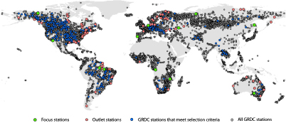
Figure 2. The spatial distribution of GRDC stations used for this study. Each dot shows a GRDC station (n = 9051) from the station catalogue. Blue dots indicate all GRDC stations (n = 471) that meet the selection criteria, whereas the red dots refer to the stations (n = 92) that are located at the outlet of a catchment. The green dots indicate those stations (n = 12) that were selected for detailed analyses.
Download figure:
Standard image High-resolution imageWe then made a distinction between near-natural and managed catchments. Following Beck et al (2016), a catchment is classified as near-natural if the share of land-area subject to irrigation is <2% and the total reservoir capacity is <10% of its long-term mean annual discharge. If these conditions were not met the catchment was classified as managed. The classification was based on the HYDE 3/MIRCA land cover dataset (Fader et al 2010, Klein Goldewijk and Van Drecht 2006, Portmann et al 2010, Ramankutty et al 2008) together with the Global Reservoir and Dam database (Lehner et al 2011). Two stations shifted from near-natural to human-impacted conditions between 1971 and 2010 and were discarded from further analysis.
The aforementioned steps resulted in 471 stations with a total catchment area covering 19.8% of the global land (figure 2), of which 92 are located at the outlet of a catchment area. The mean length of observations is 32.8 years for all stations. Of all the stations, 226 are located in managed and 245 in near-natural catchments. Of the stations located at the outlet of a catchment, 45 are managed (4.8% of the global land area) and 47 are near-natural (15.1% of the global land area).
Figure 2 shows that the majority of selected stations (blue) are located in northern and Latin America, Europe, southern Africa and Australia. The number of stations in northern and central Africa and Asia is relatively small. We selected 12 stations in river basins located in different geographic regions (green circles in figure 2: Amazonas, Amur, Colorado, Congo, Guadiana, Mackenzie, Murray, Ob, Rhine, Tocantins, Volga and the Zambezi) for which a detailed analysis is provided in the supplementary results section (supplementary).
2.3. Evaluating model performance
To evaluate the GHM simulation of monthly discharge and hydrological extremes under HIP and NOHIP conditions, we compared the modeled results with observed river discharge data using several evaluation metrics described below. To ensure a consistent comparison between the modeled and observed data, we only used modeled data for the same years for which observations were available. We also corrected modeled discharges for potential over- and underestimations caused by the difference in catchment size between the model and the GRDC. To do this, we used a multiplier that represented the difference in the upstream area as reported by the GRDC and as estimated from the DDM30 network.
First, we applied the modified Kling–Gupta efficiency index (KGE) with its sub-components: the linear correlation coefficient (rKGE), the bias ratio (βKGE) and the variability ratio (γKGE) (Gupta et al 2009, Kling et al 2012). The KGE is a widely applied indicator for the validation of hydrological performance in modeling studies at the global and regional scale and provides a good representation of the 'closeness' of simulated discharges to observations (Huang et al 2017, Kuentz et al 2013, Nicolle et al 2014, Revilla-Romero et al 2015, Thiemig et al 2013, 2015, Thirel et al 2015, Wöhling et al 2013). Moreover, use of its three sub-components enables the identification of reasons for sub-optimal model performance (Gupta et al 2009, Kling et al 2012, Thiemig et al 2013). This was achieved by estimating for each sub-parameter its distance to optimal performance, and by subsequently comparing these distances across the different sub-parameters. The statistical significance of the change in KGE outcomes due to the inclusion of HIP was tested by means of regular bootstrapping (n = 1000, p ≤ 0.05 (two-tailed)), following the method of Livezey and Chen (1982) and Wilks (2006).
Second, we applied the Nash–Sutcliffe efficiency test (NSE, Nash and Sutcliffe 1970) to evaluate the representation of Q1 (high-flow) and Q99 (low-flow) conditions (e.g. Beck et al 2017a, Blösch et al 2013, Hejazi and Moglen 2008, Mohamoud 2008), obtained under fixed threshold level settings (van Loon 2015). By means of a two-sample Kolmogorov–Smirnov (KS) test (Massey 1951, p ≤ 0.05) we tested how often HIP leads to significant changes in the fit of the full modeled exceedance probability curve for hydrological extremes compared to the full observed exceedance probability curve.
3. Results
3.1. Validation and influence of human impact parameterization on overall model performance
Including the parameterization of human impacts in the GHMs leads to a large improvement in overall model performance. The hydrological performance under the HIP simulations shows a significant improvement compared to the NOHIP simulations for between 40.8% and 72.3% of the land area studied, depending on the GHM (figure 3(a)). For most GHMs, the positive effects of including HIP in the simulations outweigh the negative effects. This is the case for both near-natural and managed catchments, although the positive effects are more pronounced for the managed catchments (figures 3(a)–(d)). Near-natural catchments are only indirectly impacted by HIP, for example by receiving improved or altered water simulations from upstream managed catchments. The KGE sub-components show significant improvement in performance in large shares of the land area studied, especially for the bias and variability ratio. The bias ratio improves significantly for 36.1%–73.0% of the total land area for all catchments, compared to 64.8%–90.6% and 24.3%–70.4% in managed and near-natural catchments respectively (figure 3(b)). For the variability ratio, improvements were found for 31.4%–74.4% of the land area for all catchments (48.9%–92.6% for the managed, 23.0%–73.2% for the near-natural) (figure 3(c)). The lowest improvements are found for the correlation coefficient, with improvements for 15.9%–58.1% of the total land area for all catchments (22.1%–75.1% for the managed, 13.9%–61.4% for the near-natural) (figure 3(d)).

Figure 3. Global weighted-mean (improvement ('+') or deterioration ('−')) in the representation of hydrological performance due to HIP for all catchments, managed catchments and near-natural catchments. Figures 3(a)–(d) visualize for each GHM the share of land area with a significant change in overall hydrological performance due to the inclusion of HIP. Figures 3(e)–(h) indicate the globally weighted-mean hydrological performance after the inclusion of HIP. On each box, the red mark indicates the median. The bottom and top edges of the box indicate the 25th and 75th percentiles of the model ensemble, respectively.
Download figure:
Standard image High-resolution imageThe results are shown for each station in figure 4 for the overall model performance (KGE), and in supplementary figure 1 for the KGE sub-parameters. The results show particularly strong improvements in overall performance in Latin America, southern Africa and the northwest US. There are only a limited number of stations for which the inclusion of HIP leads to a significant decrease in overall hydrological performance for the majority of GHMs or where no to limited changes occur, for example in near-natural areas (e.g. the Amazonas).
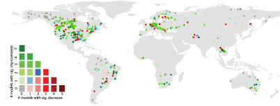
Figure 4. The number of GHMs with a significant improvement or deterioration in overall hydrological performance (KGE) due to the inclusion of HIP. The figures for the underlying KGE sub-parameters (bias ratio, variability ratio, correlation coefficient) are presented in supplementary figure 1; supplementary figure 2 shows the KGE performance values per GHM under HIP conditions.
Download figure:
Standard image High-resolution image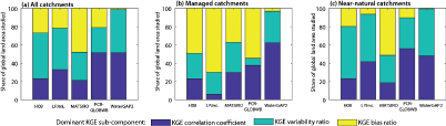
Figure 5. The share of the land area with the dominant contribution of the different KGE sub-components (KGE correlation coefficient, KGE variability ratio, KGE bias ratio) to sub-optimal overall hydrological performance under HIP conditions. Supplementary figure 3 shows per model the spatial distribution of dominant KGE sub-components.
Download figure:
Standard image High-resolution imageWhen considering overall hydrological performance for each GHM under HIP conditions (figure 3(e)), WaterGAP2 and MATSIRO show the best performance globally. Even though the simulations with HIP include human impact parameterizations by definition, all GHMs still show better performance in near-natural catchments than in managed catchments (figures 3(e)–(h)). The KGE bias ratio values >1 indicate that all models systematically overestimate long-term mean monthly discharge (figure 3(f)), up to five-fold for LPJmL in managed catchments. For the variability ratio (figure 3(g)), WaterGAP2 is the only GHM that tends to slightly underestimate variability (variability ratio <1) in the monthly discharge, in both the managed and near-natural catchments. All other GHMs show overestimations, up to 1.55 fold for LPJmL for near-natural catchments. All GHMs show a reasonable correlation with the observed monthly discharge estimates (figure 3(h)), with values ranging between 0.49–0.69 in the managed catchments and 0.50–0.79 in the near-natural catchments. The highest correlation coefficients including HIP are found for WaterGAP2, with a global mean value across all catchments of 0.76 (0.69 for the managed catchments and 0.78 for the near-natural catchments).
For each catchment (and therefore its associated land area), it is possible to distinguish which of the KGE sub-parameters contributes most to sub-optimal performance. These results are summarized in figure 5. The results show that under HIP conditions, the bias ratio contributes most to sub-optimal performance in managed catchments for most GHMs, except WaterGAP2 (for which the correlation coefficient contributes most). For near-natural catchments, sub-optimal performance is most often caused by the variability ratio for H08, LPJmL and WaterGAP2, by the bias ratio for MATSIRO and by the correlation coefficient for PCR-GLOBWB.
Spatially explicit results vary per GHM and are shown in supplementary figure 3. The distribution of dominant contributors to the sub-optimal overall hydrological performance is similar for H08, LPJmL, and PCR-GLOBWB. For these GHMs, we find dominant contributions from the bias ratio in southern Africa, Australia and inland US, and dominant contributions of the variability ratio and the correlation coefficient in Latin America as well as at higher latitude and altitude regions. For Europe, the dominant contributions for H08, LPJmL and PCR-GLOBWB are the variability ratio, the correlation coefficient, and the bias ratio respectively. The dominant contributors that cause sub-optimal overall hydrological performance for MATSIRO and WaterGAP2 are more equally distributed across the globe. While all sub-components contribute to sub-optimal overall hydrological model performance for MATSIRO, it is predominantly the correlation coefficient and the variability ratio that determines the sub-optimal performance in WaterGAP2.
3.2. Validation and influence of human impact parameterizations on the simulation of hydrological extremes
The inclusion of HIP in the simulations affects the ability of GHMs to estimate hydrological extremes correctly in the majority of the land area studied (figure 6). The inclusion of HIP leads to better model performance for all GHMs, across a substantial share of the land area studied (figures 6(a)–(b)). For high-flows, HIP improves model performance significantly across 34.6%–77.0% of the land area for all catchments (36.4%–94.7% for managed, 24.1%–79.2% for near-natural). For low-flows, HIP improves model performance significantly across 39.4%–80.4% of the land area for all catchments (29.3%–81.8% for managed, 42.7%–90.3% for near-natural). The KS-test results (supplementary figure 4) show that HIP only leads to significant changes in the representation of the exceedance probability curve in a limited number of cases for H08 and LPJmL (up to 14.1% of the land area studied), predominantly in managed catchments.
Table 1. The performance metrics used in this study and their calculation procedure. Here, si and oi are the simulated and observed monthly discharge at station i; μs and μo are the simulated and observed mean monthly discharge at station i; σs and σo are the standard deviation of the simulated and observed discharge at station i, respectively; Qs and Qo are the simulated and observed hydrological extremes.
| Abbreviation | Name | Calculation procedure | Range and ideal value |
|---|---|---|---|
| KGE | Modified Kling–Gupta efficiency index |  |
−∞ – 1 (ideal value: 1) |
| rKGE | KGE correlation coefficient (Pearson) |  |
−1 – 1 (ideal value: 1) |
| βKGE | KGE bias ratio | βKGE = μs,i/μo,i | 0 – ∞ (ideal value: 1) |
| γKGE | KGE variability ratio |  |
0 – ∞ (ideal value: 1) |
| NSE | Nash–Sutcliffe model efficiency | 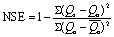 |
−∞ – 1 (ideal value: 1) |
| Q1 | High-flow indicator | Monthly discharge (m s−3) that is exceeded on average in 1 out of 100 months | |
| Q99 | Low-flow indicator | Monthly discharge (m s−3) that is exceeded on average in 99 out of 100 months | |
| KS | Two-sample Kolmogorov–Smirnov test | [h, p] = kstest2 (cdf (Qs,), cdf (Qo), 'Alpha', 0.05)a | For p > 0.05, H0 (the two cdfs coming from the same distribution) is not rejected. |
aThe calculation procedure for the two-sample Kolmogorov–Smirnov test presented in the table is the Matlab function for the KS-test.
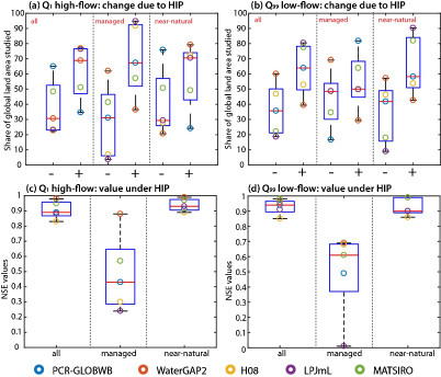
Figure 6. Global weighted-mean (improvement ('+') or deterioration ('−')) in the representation of hydrological extremes (Q1 high-flow and Q99 low-flows) due to HIP, for all catchments, managed catchments, and near-natural catchments respectively. On each box, the red mark indicates the median. The bottom and top edges of the box indicate the 25th and 75th percentiles of the model ensemble, respectively.
Download figure:
Standard image High-resolution imageOverall, hydrological extremes are represented reasonably well under HIP conditions, with globally weighted mean NSE values ranging between 0.8–0.98 for high-flows, and 0.84–0.98 for low-flows (figures 6(c)–(d)). However, there is a significant difference in the ability of the GHMs to represent hydrological extremes between managed and near-natural catchments.
Figure 7 indicates that for the majority of stations, the inclusion of HIP leads to an improvement in the representation of hydrological extremes, for most GHMs. A deterioration in the representation of hydrological extremes across the majority of GHMs as a result of the inclusion of HIP was only found in selected areas, for example at higher latitudes and along the east coast of the US. When comparing the results for Q1 high-flows with Q99 low-flows, no large differences in the spatial distribution of the number of GHMs are found with a significant improvement or deterioration.

Figure 7. The number of GHMs with a significant improvement or deterioration in the representation of hydrological extremes due to the inclusion of HIP.
Download figure:
Standard image High-resolution image
The effects of HIP on the magnitude of extreme discharge differ for low-flows and high-flows (supplementary figure 5). Whilst the magnitude of high-flows mostly decreases with the inclusion of HIP, the effects on the magnitude of low-flows are both positive and negative. The convergence of results towards higher observed discharges, in both high- and low-flow estimates (as identified for all models in supplementary figure 5), indicates that HIP becomes less important for the correct representation of hydrological extremes with increasing discharge volumes.
4. Discussion
Our results show that including HIP in GHMs generally improves the overall hydrological performance of the GHMs, as well as their representation of hydrological extremes. However, we also show that further improvements are needed. In this section, we discuss: (1) possible reasons for the improved model performance due to HIP; (2) the main limitations of the current modeling frameworks and their representation of HIP, as well as potential ways to improve them; and (3) we reflect on the general limitations in the current study design and provide suggestions for further research.
4.1. Improvements in model performance due to HIP and challenges ahead
Whilst the inclusion of HIP predominantly leads to the largest improvements in simulated discharge in the managed catchments, simulated discharge is also improved in a large share of the near-natural catchments. Improvements in model performance associated with the inclusion of HIP can be attributed to improvements in the different KGE sub-components, and in turn to different model components parameterizing hydrological and human processes. In addition, insights into those factors bounding the optimal hydrological model performance under HIP conditions may help to identify priorities for further model improvement.
4.1.1. Representation of long-term mean discharges (bias ratio)
Our study shows that the representation of long-term mean discharges significantly improved with the inclusion of HIP, especially in the managed catchments. The inclusion of HIP generally results in lower simulated discharges. As most GHMs systematically overestimate river discharges in the NOHIP simulation, this results in an improved performance. When HIP is included, we only find a deterioration in the bias ratio in selected higher latitude/altitude regions, where discharges are underestimated; this finding is in line with the outcomes of single-model studies performed by Döll et al (2009), De Graaf et al (2014) and Haddeland et al (2006). Improvements in the bias ratios due to the inclusion of HIP can be attributed to the inclusion of water abstractions and return flows (supplementary table 1B–G), and the incorporation of irrigated areas and irrigation rules, which influence evapotranspiration rates and the generation of runoff (supplementary table 1E).
However, despite improvement in the bias ratio with the inclusion of HIP, this KGE sub-indicator contributes most to sub-optimal performance in managed catchments for H08, LPJmL, MATSIRO and PCR-GLOBWB under HIP conditions. As the GHMs continue to overestimate long-term mean discharges in most cases under HIP conditions, future model improvements should target the correction of this bias in these locations. This may be achieved by critically revisiting the methods used to represent evapotranspiration rates (supplementary table 1A), runoff generation processes (supplementary table 1A) and the level of water abstractions in managed catchments (supplementary table 1B–E). The relatively good performance of WaterGAP2, in which biases in long-term mean annual discharge are adjusted using a parameter that determines the portion of effective precipitation that becomes surface runoff (Müller Schmied et al 2014), highlights the potential importance of including a calibration routine (supplementary table 1I). Calibration is also performed for H08, but this calibration routine aims to minimize runoff bias by modifying two parameters of subsurface flow for four climatic groups (Hanasaki et al 2008a, 2008b); it is therefore less effective at minimizing the bias ratio under HIP conditions.
4.1.2. Representation of hydrological variability (variability ratio)
The inclusion of HIP leads to mixed results regarding the representation of hydrological variability. Whilst HIP improved the representation of variability in some catchments and for some GHMs, it deteriorated the representation of variability for others. For example, it led to improvements in the west coast US, southern Africa and Australia, but a deterioration for most GHMs in Europe and inland US. Similar results were found by Biemans et al (2011), De Graaf et al (2014) and Masaki et al (2017) for a selection of catchments. Changes in the variability ratio due to the inclusion of HIP are predominantly driven by the timing of water abstractions and return flows, as well as by reservoir operation rules (supplementary table 1F–H). These human activities influence the relative size of high- and low-flows compared to their long-term mean discharge values.
The variability ratio is the KGE sub-parameter that contributes most to the sub-optimal performance in near-natural catchments with the inclusion of HIP, for H08, LPJmL and WaterGAP2. These GHMs significantly overestimate hydrological variability in near-natural catchments (except WaterGAP2, which underestimates variability in managed and near-natural catchments), and model improvement should therefore focus on better representing the speed of hydrological response, e.g. through an improved representation of the soil moisture storage capacity or the ratio between surface and sub-surface runoff (supplementary table 1A). In those cases where the variability ratio is also the KGE sub-parameter that contributes most to sub-optimal performance in managed catchments, model improvement should target the timing of water abstractions, return flows and reservoir management (supplementary table 1F–H).
4.1.3. Representation of the goodness-of-fit (correlation coefficient)
The inclusion of HIP only led to improved correlation coefficients in limited cases, and often resulted in a deterioration, even in managed catchments. Correlation coefficients between observed and modeled discharges, which are predominantly determined by the hydro-meteorological forcing data (Döll et al 2016, Beck et al 2016), were found to be generally high under both HIP and NOHIP conditions. Perturbations of the hydrological cycle due to human activity leading to changes in the timing of discharges and in the shape of the hydrograph, like return flows and reservoir operations, explain the observed decrease in the correlation coefficient in a substantial share of catchments and models globally (supplementary table 1F–H).
Under HIP conditions, the correlation coefficient is the KGE sub-parameter that contributes most to sub-optimal performance only in PCR-GLOBWB for near-natural catchments and WaterGAP2 for managed catchments. It should be acknowledged, though, that correlation coefficients for PCR-GLOBWB and WaterGAP2 are relatively high, especially compared to the other GHMs. The relatively low correlation coefficients in near-natural catchments found at higher latitudes in all models may be addressed by critically reviewing the snow accumulation and melt processes in the GHMs (supplementary table 1A). Higher correlation coefficients in the managed catchments may be established by improving the timing and quantification of return flow estimates and the representativeness of reservoir operations (supplementary table 1F–H).
4.1.4. Representation of hydrological extremes
The inclusion of HIP also led to significant changes in the ability of most GHMs to represent hydrological extremes (both high- and low-flows), although the strength of this change is very much dependent on the location and GHM in question. Whilst the magnitude of high-flow estimates mainly decreased due to the inclusion of HIP, low-flow estimates showed mixed results. This is because the impact of human activity tends to be greater for lower discharges, as the relative 'size' of human perturbations (such as water abstractions, return flows or delayed releases of water via reservoir operations) is higher as a percentage of the overall discharge when flows are low. Both De Graaf et al (2014) and Wada et al (2013a) found similar results when investigating hydro-climatic extremes. However, even with the inclusion of HIP, the representation of hydrological extremes is sub-optimal. Future model improvements should aim to better characterize these extremes and to improve the representation of human activity during extreme hydrological conditions.
4.2. Limitations and further research
As the GHMs have very different parameterizations of hydrological and human processes, the current study does not allow a systematic assessment of specific cause–effect relations between HIP and the observed improvements in performance (Döll et al 2016, Haddeland et al 2014, Hagemann et al 2013, Schewe et al 2014, Beck et al 2016). To do this, a substantial Monte Carlo analysis would be required, whereby individual parameters and combinations of parameters are systematically modified for all GHMs (Döll et al 2016). Undertaking such an analysis in parallel to the different GHMs incorporated is computationally expensive and requires a strict modeling protocol. It may, however, provide additional information on how to adapt and improve the individual GHMs and would be a valuable addition to the results presented in this study.
When interpreting the results of this study, one must take into account that we only evaluated the GHMs with respect to the monthly discharge. Whilst the monthly discharge may be sufficient for the assessment and management of low-flows, droughts and freshwater resource availability, flood risk assessment and management require information on the daily peak discharge. Further research should therefore attempt to validate GHMs using daily peak discharge and assess how it is affected by the inclusion of HIP.
The spatial resolution of the GHMs applied in this study is 0.5° × 0.5° (~50 km × 50 km at the equator), dictated by the resolution of the GSWP3 input dataset. At a 0.5° × 0.5° spatial resolution, hydrological processes are often represented by GHMs in a simplified or generalized form which are not fit for local applications (Bierkens 2015). To account for this, we applied a minimum catchment size of 9000 km2, thereby omitting catchments that are too small to be adequately represented by GHMs (Hunger and Döll 2008). Newer versions of several of the GHMs now operate at higher resolutions; for example WaterGAP and PCR-GLOBWB have recently been published in 5 m/6 m versions respectively (Verzano et al 2012, Wada et al 2016b). Future research can investigate whether the inclusion of these high-resolution model-runs improves the representation of discharges and hydrological extremes in the selected catchments and whether these high-resolution runs also allow for the inclusion of smaller catchments.
In this study, a relatively simple distinction was made between managed and near-natural catchments using two parameters: irrigated agriculture and reservoirs. These parameters were chosen as they have been reported to be the most significant human parameters on river hydrology (Beck et al 2016, 2017a). However, to make a more detailed distinction between catchments that are impacted by human activity and those that are not, future studies could consider incorporating additional criteria, such as the share of sectoral water abstractions and return flows, and the share of built-up land area. Additional catchment descriptors (Eisner 2016), like climate conditions and the physiographic properties of the drainage area, could also be applied to further assess the important controls on modeled discharges.
When evaluating the impact of HIP on hydrological extremes, we only incorporated results for the Q1 high-flow and Q99 low-flow. In this study, we did not consider other ranges of the extreme value distribution explicitly. Although the inclusion of HIP influences these hydrological extremes substantially, we found very few instances for which this led to a significant change in the full exceedance probability curve. Future research should therefore also incorporate other ranges of the probability exceedance curve in order to do a full assessment of the influence of HIP on high- and low-flow extremes.
Next to the parameterizations and representation of hydrological processes and human impacts, other sources contribute to uncertainty in the modeling of discharges and hydrological extremes. These include the quality of the data, the uncertainties in the input data and observation datasets and the calibration/validation strategy (Döll et al 2016, Sood and Smakhtin 2015). The quality of the selected forcing data, for example, may limit the representation of monthly discharges and hydrological extremes significantly (Döll et al 2016, Beck et al 2016), although this not been evaluated explicitly here. However, climate forcing uncertainty is probably a dominant driver for model outputs (Müller Schmied et al 2014, 2016). Benchmarking of the GSWP3 dataset against historical observations of precipitation and temperature, or against other forcing datasets (e.g. similar to Beck et al 2017b, Sun et al 2018), may therefore be of added value.
Differences in the quality and trustworthiness of the historical discharge observations (e.g. due to sampling, measurement and interpretation errors), may potentially result in artificial biases in the validation results (Renard et al 2010). The spatial representativeness of our results is limited by the availability of consistent publicly available in situ observations of sufficient quality. Future research should therefore consider extending the GRDC data-points to the regional repositories of observed discharges, as recently attempted by Beck et al (2016), Do et al (2017) and Gudmundsson et al (2017). However, increasing spatial representation comes at the cost of consistency, and special attention should be paid to the harmonization of these different databases. The use of remotely sensed data could also provide a valuable way of carrying out calibration and validation in ungauged regions (Döll et al 2014a, 2014b, Scanlon et al 2018). Remotely sensed data can also be of added value in the assessment of water consumed by agricultural irrigation (Peña-Arancibia et al 2016), operational drought monitoring and early warning (Ahmadalipour et al 2017), as well as the estimation of terrestrial water budgets (Zhang et al 2017). Moreover, clear potential exists for assimilating remotely sensed data into the models (Eicker et al 2014).
Calibration and validation are essential to compensate for factors such as the impossibility of measuring all required model parameters at the applied scale, the lack of process understanding, the simplistic process representation in GHMs and errors in forcing data (Beck et al 2016, Bierkens 2015, Döll et al 2016, Liu et al 2017). Hence, calibration/validation is key for obtaining realistic model performance. It should be acknowledged, though, that the representation of hydrological and/or human processes is artificially altered by means of calibration/validation processes and that limited calibration may introduce uncertainties to the model output (Sood and Smakhtin 2015). Before using any calibrated/validated model data, one should therefore critically reflect on whether the calibration/validation procedure executed—together with their optimization objectives—are fit for the specific application in mind.
5. Summary and conclusions
This study shows that the inclusion of human activity in GHMs can significantly improve the simulation of monthly discharges and hydrological extremes, for the majority of catchments studied. The finding is robust across both managed and near-natural catchments. The global and spatially distributed results presented in this study indicate that the inclusion of human impact parameterizations (HIP) is associated with improvements in the bias ratio and the variability ratio. Whilst the biases in long-term mean monthly discharge decrease significantly in 36.1%–73.0% of the studied catchments due to the inclusion of HIP, the modeling of hydrological variability improves significantly in 31.4%–74.4% of the catchments. Estimates of hydrological extremes are also significantly influenced by the inclusion of HIP, although the influence is highly dependent on the location and GHM in question. While HIP generally leads to a decrease (and thus improvement) in the absolute magnitude of simulated high-flows, its impact on low-flows is mixed.
Even when human activity is included in GHMs, their performance is still limited; this is particularly the case in managed catchments. Moreover, the systematic misrepresentation of hydrological extremes across all GHMs calls for a careful interpretation of risk assessments based on their results, and further study into the overarching research theme of water resources, hydrological extremes, human interventions, and feedback linkages. The large variation in performance between GHMs, regions and performance indicators, highlights the importance of carefully selecting models, model components and evaluation metrics in future model applications. For example, for a study of droughts it is essential to correctly represent hydrological variability, whilst to study water scarcity it is crucial to minimize biases.
Sub-KGE results, which were presented in this study for each GHM, allow for the attribution of different hydrological and human impact model-components limiting optimal hydrological performance. In most GHMs, model performance is limited due to the overestimation of long-term mean discharges. The correlation coefficient is the limiting factor for optimal model performance for WaterGAP2, despite the high correlation coefficients that were found for this model relative to the other GHMs studied. A better understanding of these factors, as provided by this study, may assist in the identification of priorities for further model improvement.
Acknowledgments
The Global Runoff Data Centre (GRDC, 56068 Koblenz, Germany) is thanked for providing the observed discharge data. This work has been conducted under the framework of phase two of the Inter-Sectoral Impact Model Intercomparison Project (ISIMIP2a: www.isimip.org) and the authors want to thank the coordination team responsible for bringing together the different global hydrological modeling groups and for coordinating the research agenda, which resulted in this manuscript. The research leading to this article is partly funded by the EU 7th Framework Programme through the project Earth2Observe (grant agreement no. 603608). JZ was funded by the Islamic Development Bank. PJW received additional funding from the Netherlands Organisation for Scientific Research (NWO) in the form of a Vidi grant (016.161.324). JCJHA received funding from the Netherlands Organisation for Scientific Research (NWO) Vici (grant no. 453-14-006). YM was supported by the Environment Research and Technology Development Fund (S-10) of the Ministry of the Environment.