
Modeling of German Low Voltage Cables with Ground Return Path
by
 ,
,
Johanna Geis-Schroer
1,*,† ,
,
Sebastian Hubschneider
1,*,†,
Lukas Held
1,†,
Frederik Gielnik
1,
Michael Armbruster
2,
Michael Suriyah
1 and
Thomas Leibfried
1 
1
Institute of Electrical Energy Systems and High-Voltage Technology (IEH), Karlsruhe Institute of Technology (KIT), 76137 Karlsruhe, Germany
2
Stadtwerke Buehl GmbH, 77815 Buehl, Germany
*
Authors to whom correspondence should be addressed.
†
These authors contributed equally to this work.
Energies 2021, 14(5), 1265; https://doi.org/10.3390/en14051265
Submission received: 15 December 2020
/
Revised: 11 February 2021
/
Accepted: 15 February 2021
/
Published: 25 February 2021
(This article belongs to the Special Issue Electric Distribution System Modeling and Analysis)
Abstract
:In this contribution, measurement data of phase, neutral, and ground currents from real low voltage (LV) feeders in Germany is presented and analyzed. The data obtained is used to review and evaluate common modeling approaches for LV systems. An alternative modeling approach for detailed cable and ground modeling, which allows for the consideration of typical German LV earthing conditions and asymmetrical cable design, is proposed. Further, analytical calculation methods for model parameters are described and compared to laboratory measurement results of real LV cables. The models are then evaluated in terms of parameter sensitivity and parameter relevance, focusing on the influence of conventionally performed simplifications, such as neglecting house junction cables, shunt admittances, or temperature dependencies. By comparing measurement data from a real LV feeder to simulation results, the proposed modeling approach is validated.
1. Introduction
Traditionally, distribution system operators (DSOs) assume symmetrical load conditions for low voltage grid planning [1]. Despite the single-phase connection of most domestic appliances, equal load distribution is achieved by considering wider grid segments and statistically averaging a large number of costumers. When also assuming symmetrically designed electrical equipment, this allows for modeling low voltage (LV) grids as simple, single-phase equivalent systems.
In the course of the ongoing German energy transition, the number of distributed photovoltaic (PV) systems installed in low voltage grids are rising. About 70% of those are small single- or two-phase rooftop systems [2]. Looking at this in more detail, the previously mentioned DSO’s assumption of symmetrical load conditions is not feasible anymore. Measurement results from Reference [2] show that 93% of single-phase PV inverters are connected to the same phase, typically phase a. Increasing penetration rates of electric vehicles and battery storage systems—of which, once again, a large share has single-phase or two-phase grid connections—further amplify asymmetrical load situations [3].
The discrepancy between the assumptions during grid planning and present asymmetrical grid reality causes new challenges in grid operation, for example concerning voltage quality according to European standard DIN EN 50160 or neutral conductor ampacity [4]. In order to evaluate these issues and develop potential solutions, there is a growing interest in detailed modeling of distribution grids, used for integration studies, stability studies and real-time simulation environments. Not only load modeling, but also detailed modeling of lines, is mandatory for unbalanced system studies. With a share of 80% and increasing, underground cables are the dominating line type in German LV grids [5]. The most common cable types, four-core NAYY and NAYCWY, are depicted in Figure 1.
Authors, like Oeding et al. [6], present tables for positive and zero sequence impedance parameters for different cable types, intended for rough calculations of minimum and maximum fault currents. Based on the assumption of equal mutual inductances between phases—which seems unrealistic for four-core cables (see Figure 1)—these parameters do not seem to be suitable for modeling of LV systems. Furthermore, the underlying assumptions regarding system grounding are derived from transmission grids [6] and seem questionable for German LV grids.
In this contribution, we present measurement data of phase, neutral and ground currents from real LV substations and feeders in Section 2. In Section 3, we use this data to review and evaluate common modeling approaches for LV systems. Lastly, we present an alternative modeling approach, which allows for the consideration of typical German LV earthing conditions and asymmetrical cable design. In Section 4, we present calculation methods for our cable model parameters, and validate these through laboratory measurements of real LV cables. Section 5 focuses on modeling grounding impedances at substations and costumer nodes. In Section 6, we evaluate our model in terms of parameter sensitivity and parameter relevance, focusing on the influence of commonly performed simplifications, such as neglecting house junction cables, temperature dependencies, or shunt admittance. In order to validate our modeling approach, we compare simulation results to measurement data from a real LV feeder in Section 7. Our conclusions are drawn in the final section.
2. Monitoring of Real LV Feeders
This section presents measurement data recorded in real low voltage distribution grids. The grids of two different distribution system operators in South Western Germany, Stadtwerke Buehl GmbH and Netze BW GmbH, are located in areas with different geographical characteristics. While substations A to D are located in the plain Rhine valley, substations E to H are located in the Black Forest highlands. Both grids are part of larger grid areas and include several medium voltage/low voltage (MV/LV) substations. The corresponding low voltage grids differ in line equipment (cable versus overhead line), as well as number of feeders and type of customers (residential versus industrial areas).
In the following, we show and compare results from two different types of measurements. Section 2.1 focuses on line currents of single feeders (see Figure 2a), while Section 2.2 analyzes data of current measurements at substation busbars (see Figure 2b). For acquiring measurements, we used a Tektronix 8 channel 12 bit mixed signal oscilloscope of type MSO58. Hall-effect current clamps PAC16 by Chauvin Arnoux were used for measuring the currents.
Both measurements focus on return currents through neutral conductor and ground, where ground is considered to be a return path through building foundation grounding, soil and transformer foundation grounding, marked with the subscript G in variable names. This additional return path through ground results from the TN-C-S design of the German low voltage grid (see Section 3). In this TN-C-S design, the neutral conductor is grounded at both the transformer neutral point and every customer node. The neutral conductor is usually combined with the PE (protective earth) conductor and, therefore, labeled as PEN (protective earth neutral) conductor.
2.1. Detailed Measurement of Line Currents
Figure 2a depicts the measurement scheme exemplarily for feeder 1. The three phase currents , , and and the PEN current of one single feeder are recorded at the same time. The direction of current flow is defined in direction of the substation.
2.1.1. Breakdown of Feeder Currents
Figure 3 exemplarily shows measurements of currents of all six feeders of substation D over 20 ms. For all feeders, the three phase currents (brown), (black), and (grey) are significantly imbalanced; hence, the PEN conductor is carrying the return current (blue). The residual ground current (yellow) was calculated according to Equation (1), assuming the considered feeder to be the only one at the substation (also see Section 2.3).
Table 1 shows the root mean square (RMS) values and corresponding to measured PEN currents and calculated ground currents , respectively, for several feeders in different MV/LV substations. Due to safety reasons and difficulties to access all four conductors with current clamps, measurements could not be performed at all feeders of all substations.
Besides the ratio of true RMS values, Table 1 also provides the ratio , which only considers RMS values of the fundamental oscillation. The ratio of ground currents to PEN conductor currents, , varies between 0.06 and 0.66 and is equal to or lower than —which reaches up to 0.93—for all considered feeders. This is consistent with Figure 3, where shows less harmonic distortion than for all six feeders of substation D. The difference between both ratios allows us to draw the conclusion of different loads being responsible for the ground currents in different shares.
Due to the small number of measurement samples, it is not possible to draw general conclusions regarding the influence of line type, number of cable cabinets and customers on the share of return current flowing through ground. However, the average of for feeders with more than ten costumer nodes (0.44) is noticeably higher compared to the one of feeders with less than ten costumer nodes (0.23). A possible explanation is that grounding impedances of costumer nodes provide parallel grounding resistances, which leads to a decreased overall ground return path impedance.
2.1.2. Time Dependency
Table 2 shows measurements results of substation A, feeder 2. The RMS currents and , as well as the ratio between these currents, as described earlier, are given for different times. Typical changes in phase loads—and in load imbalance—during the considered time period of 82 min led to significant variations in measured PEN current and calculated ground current . In contrast, the ratios of ground to PEN current and both remain similar over time with a relative standard deviation of 8% and 11%, respectively.
Hence, the measurement results show that a changing load situation does not lead to major changes in the ratio, which indicates a nearly rigid grounding situation and, thus, constant shares of ground currents for the considered LV feeder. We assume the remaining deviations in ratio over time to result from neutral current composition by different customers and, thus, different grounding paths and impedances.
2.2. Measurements at Substation PEN Busbars
The analysis in Section 2.1 focuses on individual feeders. This section, in contrast, focuses on measurements at the substations’ PEN busbar at the LV side of the respective MV/LV transformer. The PEN conductors of all feeders and the transformer’s neutral conductor are connected to this busbar. The current clamps were installed as depicted in Figure 2b.
Figure 4 shows exemplary measurement results from substation D. The currents of PEN conductors from Feeder 1 to Feeder 6 are described by to (grey). The sum of these currents adds to (blue). Curve (green) shows the neutral point current of the transformer.
As seen earlier for feeder currents in Section 2.1, there is a relevant deviation between the neutral point current of the transformer and the sum of the feeders’ PEN currents. The overall sum of the currents in the PEN busbar has to add to zero. Hence, the residual current , yellow in Figure 4, results from Equation (2).
Table 3 shows the RMS values of the already introduced currents , and for seven different substations B to H with 2–10 feeders and 9–111 customers. In addition, it lists the ratio to , as well as, again, the ratio of their fundamentals and . Harmonic distortion in all currents is clearly visible in Figure 4. For the considered substations, the ratios between true RMS values of ground and PEN currents range between 0.01 and 0.21. Ratios of fundamental RMS values are very similar, showing absolute differences of only up to 0.01 compared to true RMS ratios. Both ratios are significantly lower compared to the ratios calculated for single feeders in Table 1.
2.3. Conclusions
From a general point of view, the measurement data shows that power flow in German low voltage grids is typically significantly unbalanced, which leads to transformer neutral point currents of up to the same magnitude as phase currents.
Furthermore, the analysis indicates that some part of the balancing currents takes different paths than the PEN conductors, i.e., through grounding devices and soil. Considering single feeders, the theoretical ground current as residual current of phase and PEN conductor currents ranges between 6% and 93% of the PEN current. As it reduces voltage drops across the PEN conductor and influences the cable’s magnetic field, it is, therefore, relevant for detailed modeling of LV grids. The ratio between both currents is not constant, but—compared to absolute current values—only slightly differs in time. Additionally, the ratio varies between LV feeders.
The ratio ground to PEN current is typically smaller for substations than for feeders. We assume this to result from compensating ground currents between different feeders belonging to the same substation, as ground currents are not bound to physical conductors.
Considering these observations, accounting for the ground return path is significant when aiming for accurate low voltage feeder modeling.
3. Modeling Approaches of Low Voltage Cables and Grounding
When trying to accurately model line impedances in LV grids, a common problem is that DSOs do not provide detailed information about type, condition (age), and length of underground cables and overhead lines. However, even if this information is available, one main challenge remains due to the design of the German distribution network as TN-C-S system.
3.1. German LV Grid as TN-C-S System
As shown in Figure 5, there is a combined PEN conductor between the substation and the building connection point. Inside of the building, it is split up into separate PE and n conductors. The PEN conductor is grounded at the transformer neutral point, and the PE conductor—hence, indirectly the n conductor—is connected to the main earth bar in the customer buildings. Due to this, a ground return path is provided in parallel to the PEN conductor. The measurement data presented in Section 2 clearly shows the relevance of accounting for this ground return path when modeling unbalanced current flow through low voltage cables.
Modeling this ground return path is a nontrivial task, mainly because soil resistivity varies with soil type, humidity, and temperature—Table 4 gives exemplary values in comparison with non-soil materials. Furthermore, in Europe’s mainly moderate climate zone, soil resistivity values follow a sinusoidal dependency reaching their mean value in May and November, while the maximum and minimum values in April and August are approximately 30% higher and lower [11]. In addition, the realization and the effectiveness of the grounding electrode varies depending the age of the building (see Section 5).
3.2. Conventional Modeling Approaches
This subsection gives a brief overview of modeling approaches of low voltage cables in related work, presenting and evaluating underlying assumptions.
3.2.1. Handling of Shunt Admittances
Shunt admittances between cable conductors and to ground consist of conductances and capacitances. For dielectric material not being excessively aged by improper cable operating conditions, conductance G is negligibly small compared to [15]. Hence, in literature there is general agreement on neglecting conductances when modeling low voltage cables [16,17,18,19].
According to authors, like Oeding and Oswald [6], Schwab [1], and Kersting [20], capacitances cannot be generally classified as negligible in low voltage cables due to small distances between conductors and the high permittivity of polyvinyl chloride (PVC).
The authors of References [16,17,18,19], however, neglect both conductances and capacitances, pointing out that the influence of shunt admittances on voltage deltas along low voltage cables is rather small compared to the influence of line resistances and inductances. In CIGRÉ benchmark grids, neglecting capacitances is justified by referring to comparatively small line lengths in low voltage grids [21]. Since no author quantifies the exact influence of neglecting capacitances on simulated node voltages, it remains unclear whether modeling capacitances is relevant for detailed modeling of low voltage cables.
3.2.2. Temperature-Independent Parameters
As low voltage cables are usually embedded about 1 below ground surface, daily temperature variations do not influence the temperature of the surrounding soil [22]. Nevertheless, heat losses of cables in operation lead to increased conductor and insulation temperatures. Depending on the load situation, temperatures inside the cable may reach the maximum rated temperature of 70 for PVC-insulated cables [23]. The electrical conductivity of the conductor shows a significant temperature dependency [24]. However, common modeling approaches assume conductor resistance to be constant during operation, relying on reference values valid for a temperature of 20 . In literature, there has been no discussion on the effect of this simplifying assumption on simulation accuracy.
3.2.3. Modeling in Symmetrical Components
As can be seen from the most typical German four-core low voltage cable types in Figure 1, the cable design shows asymmetry. We expect that magnetic and electrical coupling, i.e., mutual inductances and capacitances, between horizontally/vertically conductor pairs significantly differ from those of diagonal conductor pairs.
However, when assuming mutual inductances to be symmetrical and applying symmetrical components, line models can be described by three-dimensional diagonal phase impedance matrices, which greatly simplify load flow calculations or impedance estimation methods [6,16,25]. Using these reduced models only requires knowledge of four parameters: line resistance and reactance in both positive and zero components. Authors, like Oeding and Oswald [6], provide tables with corresponding reference values for different German low voltage cable types, yet pointing out that these parameters are originally intended for rough calculations of minimum and maximum fault currents and, thus, not necessarily suitable for accurate modeling of low voltage grids.
Urquhart [25] demonstrates, for a British low voltage cable with similar asymmetrical design to the typical German four-core NAYCWY in Figure 1b, that, approximating the impedance matrix only in terms of positive and zero sequences, can lead to considerable errors of up to 17% in calculation of voltage drops.
Another possible source of inaccuracies with modeling in symmetrical components results from underlying assumptions with respect to grounding. Oeding and Oswald [6] present two different zero sequence impedance values for each cable type. The first one is based on neglecting the ground return path. Our analysis of measurement data from real German LV grids in Section 2 clearly shows that assuming the neutral conductor as the only return path for balancing currents is not feasible when aiming at accurate modeling of real load scenarios. The second zero impedance value provided in Reference [6] is derived from modeling the ground return path according to Carson’s approach and applying Kron’s reduction. In the following, we will briefly outline the latter approach, and evaluate its suitability for modeling of German LV grids.
3.2.4. Carson’s Equations for Ground Return Path Modeling
The classical approach for ground return path modeling starts from a five-conductor system, where a fictitious fifth conductor in parallel to phase and neutral conductors represents the ground return path (see Figure 6). There is magnetic coupling between all five conductors. The sum of currents in the cable and ground is assumed to be zero, such that:
Voltages in Figure 6 are defined relative to the transformer’s grounded neutral point, i.e., reference ground. As Figure 6 depicts a cable segment not directly connected to the transformer, and are local ground voltages of magnitudes unequal to zero. Voltage drop across the cable segment is described by Equation (4).
Primitive Circuit Impedances
Re-arranging Equation (4) for voltage differences relative to local ground voltages and using Equation (3) leads to Equation (5) [20,26], where and refer to so-called “primitive” self and mutual impedances, into which the impedance of the ground return path is merged (see Equations (6) and (7)).
Originally presented for telegraph overhead lines in 1926 [27], Carson’s equations enable to directly compute these primitive impedances. Carson assumes the soil to be of constant specific resistance and infinite in radius and depth, and models ground currents as images of conductor currents in soil. Furthermore, he assumes that conductor diameters are small compared to distances between conductors. He solves for the impedances by considering electromagnetic fields between conductors and images [25].
By only considering those terms from the original equations that are relevant at technical frequencies, Kersting [20] derives simplified equations. Transforming these into SI units leads to Equations (8) and (9) [25], which only contain the variables conductor resistance in , specific soil resistance in , grid frequency f in Hz and geometric dimensions and in m. Geometric mean radii and geometric mean distances can easily be calculated for round conductor arrangements in low voltage cables (see Section 4.2.2).
Kron’s Reduction
Using common power flow software and modeling in symmetrical components do not allow for an explicit representation of the neutral conductor [20,21,25]. The 4 × 4 system in Equation (5), thus, often needs to be reduced to a three-dimensional system. This cannot be done solely through simple transformations of equations, but requires further assumptions. Usually, Kron’s reduction is applied, which implicates assuming a perfectly grounded neutral point at every node [20,25].
In general, assuming a perfectly grounded neutral at every node clearly seems unrealistic for low voltage grids. Although there may be grounding electrodes at substations and costumer nodes, such as in the German TN-C-S system, there are most likely also nodes without grounding, such as junctions between two cable types. The authors of References [25,28], therefore, do not apply Kron’s reduction to calculated primitive impedances.
Applicability To German Low Voltage Grids
Even without using Kron’s reduction, considerable issues with applying Carson’s equations to models of German low voltage cables remain. While assumptions required for the derivation of Carson’s equations may be considered realistic for long overhead transmission lines—which have no neutral conductor, and ground is the only return path [15]—they appear questionable for comparatively short low voltage cables with closely spaced conductors.
As Carson models ground currents as images of line currents, a key assumption for applying his equations to cables is that cable and ground currents sum up to zero at any point along the cable, such as described by Equation (3). This does not allow for the possibility of ground currents following different routes than in parallel to the cable. In reality, for instance, metallic underground pipes might provide a path with a smaller impedance [17]. Moreover, Carson’s approach excludes circular ground currents between neighboring grounded nodes [25]. In reality, such circular currents can occur between buildings, substations or street lighting installations, even if these do not belong to the same feeder.
Lastly, our analysis of measurement data from low voltage substations and feeders in Section 2 shows that Carson’s hypothesis of ground currents being bound to paths in parallel to the feeder may not hold in reality. Technically, Equation (3) is used to determine the theoretical ground currents for a single feeder in Section 2.1. Following Carson’s approach, and thus assuming all theoretical return currents to reach the substation busbar, the ratios of ground to PEN currents of single feeders would correspond to the ratio of ground to PEN currents calculated for the entire substation. However, the substations ground current is considerably lower than the feeders theoretical ground currents. This indicates the presence of the previously described circular ground currents between feeders and busbars.
3.3. Alternative Modeling Approach: Ground as Single Electrical Point
Questioning the applicability of Carson’s equations to low voltage grid modeling, Olivier et al. [17] suggest fellow researchers to try out an alternative approach “for the sake of simplicity”: To model low voltage cable segments as four-line -systems, considering the ground as single electrical point, to which all grounded neutral points are connected—with or without grounding impedances.
As all grounding impedances refer to the same electrical point, independently of the grounded node’s distance to the transformer, we believe this alternative approach suggested in Reference [17] to represent earthing conditions of the German TN-C-S system more realistically than Carson’s equations. Notably, the alternative approach also allows for circular currents between grounded nodes.
The modeling approach used in our work is, therefore, based on Olivier et al. [17], and depicted in Figure 7. At the end of the line segment of length l, the neutral conductor is grounded with a grounding impedance , referring to grounding of an exemplary connected costumer building. As sketched in grey, reference ground is not defined to be the transformer’s neutral point, but we model the transformer’s neutral point to be grounded with an impedance .
To be able to assess the influence of model simplifications later in Section 6, we initially create our model to be as realistic as possible. As all four cable conductors are represented explicitly, we enable modeling unequal mutual inductances between conductors. In contrast to conventional modeling approaches, we also account for capacitances between cable conductors and stray capacitances to ground (blue).
With respect to parameters to be determined for our low voltage grid simulation models, we distinguish between the following two groups:
- Cable parameters The depicted cable parameters in Figure 7, , , , and , only depend on cable design and materials. For these parameters, we present calculation methods in Section 4.2 and evaluate these with laboratory measurements of real low voltage cables in Section 4.3.
- Ground/Ground return path Capacitance to ground , as well as impedances and , vary depending on the cable’s real installation conditions and can, therefore, not be determined through laboratory measurements. We present exemplary reference values in Section 4.2.3 and Section 5.
4. Low Voltage Cable Parameter Determination
For the alternative modeling approach presented in Section 3.3, no general reference values for parametrization of cable models are suggested in literature. Theoretically, an accurate determination of required parameters is possible through numerical analysis of the field differential equations (e.g., by using finite element method [26] or method of moments [29]). This requires not only detailed information on cable dimensions but also on the exact installation and environmental conditions—ideally, a three-dimensional soil model [25]. However, huge computational efforts seem disproportionate considering significant manufacturing tolerances, as seen in measurements. In addition, practical field conditions impede an exact ground return path modeling.
In this work, we use practical approaches for calculation of cable parameters, deriving required information from standards and data sheets by manufacturers, and present them in the following Section 4.2. Then, the resulting cable parameters are validated with data obtained by measurements of real cables, before analyzing the findings with respect to dependencies between different cable models.
Our test objects are of different types of underground cables typically used in German LV grids and summarized in Table 5. Three of these show an asymmetric four-core design (A, B, C), one has a symmetric three-core design (D).
4.1. Assumptions and Simplifications
Though aiming at a detailed model of cables, there are certain simplifications concerning cable lay length and shield we make and discuss shortly in the following sections.
4.1.1. Influence of Cable Lay Length
Due to the cable lay, the length of the individual conductors is higher than the cable length, to which impedance and admittance per-unit parameters are multiplied to. Unfortunately, neither manufacturer data sheets nor German cable standards provide information on lay lengths and corresponding correction factors. In accordance with Reference [26], we assume the influence of the cable lay to be negligible compared to other influences on the calculated parameters.
4.1.2. Idealization of the Concentric Conductor
The concentric copper conductor in cables of type NAYCWY is composed by several physically distanced copper wires (see Figure 8). As a copper band around the wires ensures conductivity between them, we consider the concentric copper conductor as ideal cylindrical electrical shield (see Figure 9b,c). We refer to the concentric conductor as shield (S), regardless of its actual functionality as PE (four-core NAYCWY) or PEN (three-core NAYCWY) conductor. The PEN sector-shaped conductor of NAYY cables is referred to as n (see Figure 1a).
4.2. Calculation of Cable Parameters
In the following, we provide approaches to calculate cable parameters based on geometric dimensions of conductors and insulation.
4.2.1. Ohmic Resistances
For economic reasons, we expect cable manufacturers to design conductors close to the maximum permissible values given in standard DIN VDE 0295 [33], which are listed as direct current (DC) resistances per unit length in for a temperature of 20 . For other temperatures , the standard defines the equation as given in Equation (10):
The specified cross-sectional areas in datasheets of cables refer to these resistance values, but do not correspond to the real geometric cross-sectional area. For shielded NAYCWY cables, the indicated cross-sectional area of the concentric conductor refers to the resistance value of an aluminum conductor with equivalent cross-sectional area. For example, the name extension “25” in type NAYCWY 4 × 50 SE/25 defines the maximum permissible DC resistance of the copper shield equal to the DC resistance of an aluminum conductor with a cross-sectional area of 25 [33].
For three-phase alternating current (AC) operation, the resistance is defined according to (11), where factors and represent the dependency on skin and proximity effect, respectively [24].
Both effects depend on the skin depth , which varies with typical cable operating temperatures between mm and mm (see Table 6). For the calculation of and , Oeding and Oswald [6] provide approximation formulas for symmetrical arrangements of three round conductors. The authors derive and from the parameter x, which puts conductor radius r into relation with skin depth . In order to apply the formulas from Reference [6] to sector-shaped conductors, we assume the radius r of a sector-shaped conductor to equal the radius of a round conductor with an equivalent cross-sectional area (see Equation (12)). Taking into account the European standard DIN EN 60228 [33] and once again assuming economic interests of the manufacturers, the real geometric cross-sectional area differs from —which is the nominal value as defined by the cable type. Shafieipour et al. [29] estimate to be about 88% of .
For , the relation between conductor diameter and distance to other conductors needs to be considered. We adapted the approximation formula provided in Reference [6] to account for asymmetrical arrangements of sector-shaped conductors. Table 6 gives an overview of calculated factors and for the cross-sectional areas in focus of our investigations.
As mentioned in Section 3.2.3, Oeding and Oswald [6] provide reference impedance values in symmetrical components. The indicated positive sequence resistances for the cable types in focus correspond to applying Equation (11) for a temperature of 20 and factors and from Table 6. Neglecting the comparatively small temperature dependency of and , we, thus, obtain Equation (13) for the AC resistance of sector-shaped conductors.
For concentric copper conductors, literature does not suggest AC reference values. However, as they consist of a multitude of small copper wires, we assume skin and proximity effect to be negligible. Hence, we assume the AC resistance to equal the DC resistance according to Equation (14).
4.2.2. Self and Mutual Inductances
As mentioned earlier, we cannot use reference values in symmetrical components nor Carson’s equations for consideration of self and mutual inductances in our models. In the following, we briefly outline how to use standard methods from References [34,35]—developed for overhead lines—in order to compute the required parameters.
In References [34,35], Grigsby and Glover calculate the magnetic flux linkage of an arrangement of several round conductors of infinite length. They assume uniform current distribution, which is a valid approach for the underground cables we focus in our work (see x in Table 6). According to Reference [6], a decrease in the magnetic flux due to skin effect only occurs for , while Reference [15] assumes relevance only for .
From the method presented in References [34,35], the inductance per unit length in results from Equations (15) and (16), which only depend on the geometric parameters geometric mean radius (GMR) and geometric mean distance (GMD) . It is to mention that we do not expect this to lead to significant model inaccuracies, as permeability of aluminum, copper, PVC, and common soil materials only slightly differs from vacuum.
To use Equations (15) and (16) on the conductor arrangements depicted in Figure 9, we need to determine the five parameters listed below. Since Carson’s equations also require the calculation of GMR and GMD, approaches for LV cables are available in literature.
| GMR | sector-shaped conductor | ||
| GMR | shield | ||
| GMD | horizontally/vertically neighboring sector- shaped conductors | three-core cable four-core cable | |
| GMD | diagonal conductors | four-core cable | |
| GMD | sector-shaped conductor–shield |
Geometric Mean Radius of Sector-Shaped Conductors
Geometric Mean Distance Between Sector-Shaped Conductors
The GMD of two sector-shaped conductors can be approximated as the distance of their rotational axes [26]. Equations (18) and (19) calculate the GMD in dependence of m, which is the conductors rotational axis’ distance to the rotational axis of the cable (see Figure 10). Urquhart et al. [26] refer to British cables according to the British standard BS 3988:197 [36], using the parameters back radius, sector depth and corner radius. Adapting the approach from Reference [26] to German LV cables, we interpret these parameters as , d and , respectively, as defined in the German standard DIN VDE 0276-603 [37]. Furthermore, summarizes the offset of the rotational axis due to the insulation thickness, where describes the thickness of the insulation layer according to Reference [37] and equals the conductors’ angle in the center of the cable—which is 90 (four-core cable) or 120 (three-core cable).
Geometric Mean Radius and Distance of the Concentric Shield
According to Reference [6], the GMD between any conductor and a surrounding concentric shield equals to the GMR of the shield, which corresponds to its radius. In NAYCWY cables, the shield is located on top of the core covering. Hence, the shield’s GMR can be computed according to Equation (21), where is the thickness of the core covering (see Figure 10).
4.2.3. Capacitances
In terms of shunt admittances, we only focus on capacitances between conductors, neglecting shunt conductances. While DC conductances can be easily approximated through DC conductivity and thickness of the insulation material, due to complicated frequency- and temperature-dependent polarization losses, this is not true for AC conductances [38]. However, conductances play a subordinate role (see Section 3.2.1) and, thus, are not further considered.
With respect to capacitances, the significant temperature dependency of permittivity of the insulation material PVC needs to be taken into account [24]. For 20 , varies between 3 and 4, depending on the exact composition of PVC. For maximum operation temperature of 70 , is approximately 8, which results in twice the capacitance value compared to the one for 20 . Due to the lack of further information, we assume a linear interpolation between those values.
Shafieipour et al. [29] show for a shielded four-core cable, comparing simple closed-form equations to finite element method (FEM) analysis, that the maximum error is around 5%. As the analysis in Reference [29] refers to conductors shaped as ideal quarter circles, we geometrically approximate sector-shaped conductors as a quarter or one third of a circle for our simplified calculations (see Figure 11).
We consider horizontally/vertically sector-shaped conductor pairs (e.g., a–b and b–n in Figure 11) as parallel plate capacitors (see Equation (22)). As there is no closed-form expression for capacitances in diagonal sector-shaped conductor pairs, derived from the FEM analysis in Reference [29], we approximate the values as shown in Equation (23).
Furthermore, in accordance with Reference [29], we consider conductor–shield pairs in four- and three-core NAYCWY cables as a quarter and one-third of a cylindrical capacitor, respectively (Equation (24)).
All conductors in operation additionally have an electrical field to ground. While, for NAYY-J cables, there are stray capacitances between all four conductors and ground, i.e., the surrounding soil, for NAYCWY cables, the field only exists between the concentric conductor—considered as ideal shield—and ground (). The electrical field limitation outside the cable is undetermined and strongly depends on environmental conditions [24]. An upward estimation is possible by assuming a limitation of the electrical field to the outer side of the cable’s sheath. The resulting values match with the general reference values of and for of 50 and 150 , respectively, that can be derived from symmetrical component modeling in Reference [6] and are, thus, utilized for our models.
4.3. Experimental Determination of Cable Parameters
As mentioned earlier, our investigations include measurements of the parameters from four real cables (see Table 5) for validation of the presented calculation approaches. Test cables A and B are of the same type with different cross-sectional areas, allowing for conclusions regarding scalability. On the contrary, cables B, C, and D are of different types with equal cross-sectional areas, thus allowing for comparison of the influence of cable designs.
Although measurements are ideally carried out on infinitely long cables laid out in a straight line in non-magnetic surroundings, this is obviously not applicable in reality. Installation and operation of measurement devices require both ends of the cable to be close to each other, in order to reduce parasitic effects and noise on long measurement lines. Thus, for practical reasons, the cables were installed in a U-bend with a spacing of approximately between the two halves of the cable. Cable length is limited by economic reasons, available space and cable handling, while an adequate minimal length is required for reducing parasitic effects at the cable ends and in order to obtain technically measurable results. During the measurements, cables B, C, and D were installed approximately above laboratory floor. Cable A was installed directly on a concrete surface.
Due to low measurement currents, compared to nominal currents of the cable, we assume the conductors’ temperature to be constant during measurement. Thus, for cables B, C, and D with a length of 25 , the temperature equals the laboratory’s ambient temperature of 20 . Cable A, which is installed outside the laboratory, was measured at an ambient temperature of 24 . For higher conductor temperatures, we injected currents of up to 400 . Temperature is measured at the conductor ends, under the sheath, with a Pt100 resistance thermometer.
4.3.1. Resistances and Inductances
Figure 12 depicts the measurement setup for acquiring resistances, as well as self and mutual inductances. Configured as a current source, the four-quadrant amplifier (4QA) APS 10,000 by Spitzenberger&Spies drives current through conductor i, while there is no current injected in conductor j. Current and the induced voltages and across the conductors i and j are measured by the power measuring device LMG500 by ZES Zimmer.
We determine the measured series resistance and self inductance of conductor i and the measured mutual inductance between conductor i and j, respectively, per unit length, according to Equations (25)–(27). In the equations, and are the self and mutual conductor inductances, respectively, while and summarize parasitic inductances due to non-optimal cable installation. The latter cannot be identified separately, thus having to be considered analyzing the results (see Section 4.4.2). Cable length in meters is described by l.
4.3.2. Capacitances
For capacitance measurements, we opted for the Omicron DIRANA dielectric response analyzer [39]. During measurement of capacitance between two conductors, the other conductors were grounded. Furthermore, the cable was installed adequately far from metal surfaces. Hence, stray capacitances are close to zero and are neglected.
4.4. Comparison and Analysis of Calculated and Measured Cable Parameters
Although aiming for a model valid for grid frequency of 50 , in general, we performed measurements in the range of 40 to 60 in order to identify potential interference at grid frequency.
The four test cables from Table 5 differ in conductor designs and cross-sectional areas. Nevertheless, for all cable types, comparing the results leads to similar relations between calculated values according to Section 4.2 and measured values according to Section 4.3. Thus, drawn conclusions apply for all cables under investigation. In the following, we present and discuss exemplary results.
4.4.1. Conductor Resistances
Figure 13 compares measured resistances to those calculated, for frequencies between DC and 57 . The calculated values are, in accordance with Section 4.2.1, derived from the German standard DIN VDE 0295 [33] and corrected for temperature deviation from 20 , skin and proximity effect (see Equations (10) and (11)). During measurements, only one conductor was loaded. The error bars consider measurement tolerance of the LMG500 and uncertainties in temperature measurement.
The figure shows that measured DC resistances of all four conductors are in good agreement with the calculated ones. For calculated parameters of AC resistances, skin and proximity effect have a rather low influence at the considered frequencies. However, there is a significant discrepancy between calculated and measured values of up to 8% at a frequency of 50 . Hence, measurement results show a stronger frequency dependency than calculated AC resistances. We assume the differences to result from eddy currents induced in unloaded neighboring cable conductors and, thus, as part of proximity effect. In Section 4.2.1, the proximity effect factor is calculated by an approach for symmetrical arrangements of three round conductors. In contrast, the measured low voltage cable in Figure 13 is composed by four asymmetrically arranged sector-shaped conductors. In addition, as only one conductor is loaded, the cable load is significantly unbalanced during measurement. We consider this discrepancy to be a potential reason for inaccurate representation of proximity effect.
For neighboring conductors, considering the large cross-section and comparatively thin insulation, the magnetic field facing the loaded conductor is approximately times higher than the one on the far side ( mm, ), which leads to strongly inhomogeneous currents in the sector-shaped conductors. Applying a contrary current on a neighboring conductor or symmetric three-phase currents to the cables led to deviations in measurement results, which supports the assumption of induced eddy currents being responsible for effective losses.
Eddy currents possibly induced in the floor and other metallic components in laboratory surroundings might also lead to increased measured resistances. Unfortunately, a more detailed breakdown is not possible, as material conductivity and dimensions cannot be evaluated reasonably.
Furthermore, Figure 13 shows—for every measured frequency—an offset of approximately 2% between conductors c and n. As measurement methods were the same for all conductors, and repeated measurements led to the same results, we assume these deviations to result from manufacturing tolerances.
For calculation of resistances, a linear temperature dependency of aluminum with a temperature coefficient of is assumed. Regarding temperature dependency of our test objects, measurement results for conductor n of test cable A show a linear dependency for three different temperatures (Figure 14). While we expected an increase in resistance of 10% compared to 24 for a conductor temperature of 48 , the measured increase is approximately 6%. This discrepancy can be explained by difficulties in accurately determining conductor temperature and maintaining a constant conductor temperature (with respect to time, as well as temperature gradients, across the cable length) due to effects of wind and solar radiation during measuring.
Summarizing, we can state that the calculated DC resistance values correspond well to those measured in real exemplary cables. However, considering asymmetric load situations, four-core cable designs, as well as non-negligible losses and resulting temperature deviations, measurement results diverge from the results of usual calculations. Hence, for detailed simulations of German LV systems, an in-detail consideration of resistance parameters is required. Particularly the influence of eddy currents induced in other conductors requires further investigations.
4.4.2. Self and Mutual Inductances
Figure 15 compares measured (dots) and calculated mutual inductances (hatched areas, Appendix A, Table A1) for test cables A, C, and D. Again, error bars refer to measurement tolerances according to the LMG500 data sheet.
Cable B only differs from C in its nonexistent shield. Subsequently, as the results of test cable B are very similar to those of cable C, measurements confirm the assumption that the nonmagnetic shield does not affect mutual coupling between sector-shaped conductors.
Nevertheless, for all test cables, the results depicted in Figure 15 show a nearly constant, slightly frequency dependent offset between measured and calculated values—the highest for test cable D, where measured mutual inductances are approximately 10% above computed ones. For both test cables B and C, deviation is approximately 3–4%. For the three-core cable D, deviation is actually negative. For self inductances (see Figure 16), we observed the same phenomena. The reasons for these discrepancies are still not clearly identifiable. Yet, there are several possible explanations:
- Stray magnetic flux Due to the finite length of test cables, stray magnetic flux at the cable ends can distort measured inductances. Nevertheless, this influence should actually become less relevant with an increasing length of the test object.
- Test cable setup As described in Section 4.3, test cables were installed in a U-bend, forming a kind of one-turn loop. This most likely leads to an increase in both self inductance and mutual coupling between the conductors.
- Laboratory environment Influences on the magnetic field due to the floor and other possibly magnetizable surfaces and components in the test cable surroundings cannot be excluded.
- Approximate formulas Equations (15) and (16) for calculation of self and mutual inductances were originally developed for round and infinitely long conductors, relatively far distanced from each other compared to their radius. Thus, for sector-shaped conductors with large cross-sectional areas and comparatively small geometric mean distances between them, the accuracy of the approximation is questionable.
Lastly, considering thermal influences, and thus comparing measurement results of test cable D at approximately 24 to results obtained at higher conductor temperatures, only insignificantly small differences in measurement results—all within the measurement tolerance range—could be detected. This validates our assumption of temperature-independent permeability of cable and soil materials.
4.4.3. Capacitances
Table 7 summarizes mean values of measured capacitances for 50 and different types of conductor pairs. Between pairs of the same type (e.g., c–n versus a–b as horizontally/vertically neighboring pairs), we could measure differences of up to 3% in the same cable. This most likely reflects manufacturing tolerance in insulation thickness. It can be stated that all measured values in Table 7 coincide with calculated ranges values in Appendix A, Table A1. This is valid regardless of the idealization of the sector-shaped conductors as ideal third or quarter circles.
As only one conductor was heated by the heat transformer, there was a temperature gradient across the PVC layers to neighboring conductors, which further complicated an accurate analysis of temperature dependency of . Nonetheless, our results confirm that temperature dependency generally is noticeable. For a temperature of the conductor of approximately 38 , we could measure an increased capacitance of approximately 6% compared to a conductor temperature of 24 .
5. Grounding Impedance of Grid Nodes
The grounding electrode at customer nodes is realized in various ways. For older buildings, grounding is often realized through metallic water and gas pipes entering the ground. For new buildings, in Germany it is mandatory to install a ring of stainless steel strip or round steel in the external walls of the building foundation as a foundation grounding electrode [40]. Hence, estimating a grounding system’s impedance depends on a multitude of parameters and differs between buildings. However, some general assumptions can be made, and are presented in the following sections.
5.1. System Identification and Parameter Definition
Generally, the impedance triangle depicted in Figure 17 is valid for any grounding system. Resistance and reactance refer to the grounding conductor, which connects a building’s main earth bar to the metallic grounding electrode (see Figure 5). The impedance of the metallic grounding electrode is represented by and . The complex grounding impedance is, thus, calculated as
The reactive component in Equation (28) is the sum of the grounding conductor’s reactance and the reactance of the metallic grounding electrode (see Figure 5). This reactance only needs to be considered when analyzing high frequency transients, such as those caused by lightning and switching surges, and is—compared to the resistive component —negligible at 50 [13].
The resistive component consists of the grounding conductor resistance , the metallic grounding electrode resistance and the so-called propagation resistance . The latter describes how efficient the grounding system can transmit the current and, thus, models the resistance between the earthing electrode and the reference ground. Hence, depends on the soil resistivity , as well as the type and the geometric dimensions of the grounding electrode [13].
As and are negligible compared to [13], and further neglecting the reactive component , we model the grounding impedance as approximately equal to :
5.2. Grounding Impedance of Typical Households
As stated in Section 1, due to material, temperature, and humidity variations, among others, there is a significant uncertainty in determining the value of . Therefore, it does not seem reasonable to calculate grounding resistances for different types of grounding systems and environmental conditions in detail. In order to get a reference value for simulation models, is determined for the foundation electrode of a typical German single family house with foundation dimensions of [42]. Approximate formulas for grounding resistance calculations are specified in References [41,43]. In both cases, is proportional to (see Table 8). Thus, we assume a standard value of [11].
Equation (30) from Reference [43] uses the approximation of a hemispherical grounding electrode. Variable d corresponds to the diameter of a sphere of equal volume. Applying Equation (30) to the previously described example leads to a value of (Table 8).
The authors of Reference [41] base their formula, Equation (31), on calculations for soil-embedded circular ring electrodes. The correction factor 1.05 takes into account that the foundation electrode is embedded in concrete. Concrete is less conductive than the surrounding soil. The geometrical constant g accounts for the influence of grounding electrode design and distance from the terrain surface. In order to determine g, a few more parameter values (e.g., thickness of the stainless steel strip and depth below the frost line) need to be known. Using exemplary values from Reference [41] leads to a resistance of (Table 8). For the sake of simplicity, and as an exact value cannot be found, for our models, we assume an average grounding impedance at costumer connection points to equal .
5.3. Grounding Impedance of Substations
As depicted in Figure 7, in the approach presented in the present article, the neutral point of the substation transformer is not modeled as “perfectly grounded”, but with an impedance . For this impedance, we assume a value of 2, as DSOs usually consider a grounding impedance of 2 as sufficiently low when designing MV/LV-substation grounding systems.
6. Parameter Relevance and Sensitivity
In order to evaluate the approach’s parameter relevance and sensitivity to parameter changes, we integrated our modeling approach in the simulation of a test feeder in MATLAB/Simulink.
6.1. Setup of Test Feeder Model for Parameter Analysis
Figure 18 depicts the layout of the simulated LV feeder, which is based on feeder A-2 (see Section 6, Table 1). Having a total length of more than 1 , feeder A-2 classifies as “extremely weak” according to the analysis of German LV grids in Reference [7]. Therefore, we expect significant voltage asymmetry under unbalanced load conditions.
6.1.1. Modeling of Transformer, Cable Segments and Grounding
Since our analysis focuses on modeling of cable segments and grounding impedance, we model the transformer as an ideal three-phase 230 , 50 voltage source. Its neutral point, and thus the LV PEN busbar, is grounded with an impedance of (see Section 5.3). As suggested in Section 5, foundation grounding of costumer nodes is modeled through an impedance of .
Usually, voltage drop across house junction cables is neglected when modeling and simulating LV feeders [7,25]. As outlined in Figure 18, we explicitly model house junction cables in the reference scenario, which allows for comparing the effect of other model simplifications and parameter variations to the effect of neglecting house junction cables (see Section 6.2.2). The cable segments are modeled according to Section 3, Figure 7 as four-line -model, and model parameters calculated according to Section 4. The line between nodes 1 and 2 is modeled as a cable of type NAYCWY 3 × 150 SE/95.
6.1.2. Modeling of Load Distribution
By an unbalanced assignment of six single-phase PV feed-ins (four to phase a, two to phase b) and one single-phase electric vehicle (EV) charging process at phase c in addition to the base load of costumer nodes, we induce a significantly asymmetrical load scenario (see Table 9). Since the active power values of correspond to the maximum permitted single-phase active power load or feed-in according to German DSO grid codes [44], the scenario may be considered “worst-case”, but not necessarily unrealistic.
In the reference scenario—modeled with the new detailed modeling approach as described in the previous paragraphs, without any parameter variations or model simplifications—line-to-neutral voltages at the farthest costumer node, node 19, are calculated to pu, pu and pu. Hence, according to European standard DIN EN 50160 [45], the voltage of phase a is outside the permitted voltage range of pu to pu.
Considering current magnitudes, due to the load situation, neutral current 81 in the cable segments between node 1 and 3 is higher than the phase currents , and , which is a typical current distribution for highly unbalanced load conditions. Ground current through the transformer’s grounding impedance is 10 , thus equaling approximately 11% of neutral current , which is in accordance with our field measurements (see Section 2).
In the following, we analyze the changes of simulation results relatively to the results of the reference scenario, varying cable and ground return path modeling.
6.2. Modifications in Modeling the Cable Components
Figure 19 plots line-to-neutral phase voltages at node 19 in the reference scenario as solid horizontal lines. Simulated voltages of scenarios S1 to S4 are plotted as dots, each scenario referring to a simulation with a modification in cable models. In the following, only magnitudes of currents and voltages are considered.
6.2.1. Neglecting Electrical or Magnetic Coupling between Conductors (S1a, S1b)
In the reference scenario, the currents flowing through capacitances between conductors are in the range of a few . Removing those capacitances, and thus the electrical coupling, from the model (scenario S1a), the resulting missing reactive power compensation leads to a slight increase of inductive reactive power feed-in of approximately 25 var at node 1. At node 19, compared to the reference scenario, a negligible difference in phase voltages occurs.
However, a change in phase voltages of up to pu is visible for scenario S1b, where mutual inductances, and thus the magnetic coupling between conductors, have been removed. Remarkably, the order of phase voltages also changes such that exceeds in this scenario only.
6.2.2. Neglecting House Junction Cables (S2)
For scenario S2, all house junction cables are removed from the model. Due to resulting omitted line losses, active power feed-in at node 1 is decreased by approximately 40 per phase. Furthermore, there is a slight decrease in voltage asymmetry at node 19. With an increased phase voltage of approximately pu, the biggest change is visible for phase b.
6.2.3. Variation in Conductor Temperature (S3a, S3b)
Scenarios S3a and S3b are used to assess the relevance of considering higher conductor temperatures. During summer and for load currents equal to around 50% of rated conductor currents, conductor temperatures of 30 , assumed for scenario S3a, are quite common [23]. As shown in Figure 19, changes in phase voltages at node 19 are of the same magnitude as those neglecting house junction cables in scenario S2, only now increasing voltage asymmetry due to higher conductor impedances. Since the impedance of the neutral conductor also increases, current through ground return path, , increases by approximately 4%.
As a worst-case assessment, scenario S3b assumes that all conductors in all cable segments have a temperature of 70 , typically the maximum rated temperature. This leads to a 3% increase in phase voltages at node 19, and a significant rise in voltage asymmetry. In scenario S3b, voltage falls below power quality limits defined in the European standard DIN EN 50160 [45].
6.2.4. Modifications in Modeling the Ground Return Path (S4a–S4c)
In the following, we analyze the influence of customer node and transformer grounding impedances. For scenario S4a, all grounding impedances have been deleted from the model. Thus, the neutral conductor is the only remaining return path and 0 A. This leads to increased asymmetries in node voltages, as the voltage drop across the PEN conductor rises— drops by pu, while and rise by pu and pu, respectively.
Decreasing from to in Scenario S4b—which is a typical value for urban areas with many foundation grounding electrodes close to each other [11]—does not influence simulated voltage levels much. However, decreasing from to (S4c) leads to slightly smaller voltage deltas along the lines.
6.3. Modifications in Connection Phase
Lastly, we assess how interchanging loads between phases a, b and c effects overall simulation results. Therefore, we define four different load configuration scenarios (see Table 10). K0 corresponds to the load distribution introduced in Table 9, Section 6.1.2, and is considered as base scenario. In scenarios K1, K2 and K3, loads are connected to the same costumer nodes, but to different phases. For scenario K2, the base scenario’s load allocation to phases is shifted in a circular manner; thus, the phase sequence remains equal. In contrast, K1 and K3 are two permutations with reversed phase sequence.
All scenarios K are simulated for both, a symmetrically designed feeder—all line segments modeled as symmetrically designed three-core NAYCWY cables (see Section 6.3.1)—and a feeder composed by asymmetrically designed NAYY-J four-core cables only (see Section 6.3.2).
6.3.1. Line Model: Symmetrically Designed NAYCWY Three-Core Cable
Figure 20a shows the simulated voltage magnitudes for using symmetrical NAYCWY three-core line models. Here, again, colored dots indicate the voltage levels , and at node 19 of the previously introduced feeder (see Figure 18).
For the scenarios with similar phase sequences, K0 / K2 and K1 / K3, voltage magnitudes remain at the same level. However, comparing the results from these two groups, differences in voltage magnitudes can be observed. We assume this to be due to phase currents adding up differently in the neutral conductor for different phase sequences. This leads to different voltage drops across the neutral conductor and, thus, to different magnitudes in phase–neutral voltages.
6.3.2. Line Model: Asymmetrically Designed NAYY-J Four-Core Cable
Figure 20b shows the simulated voltage magnitudes for using asymmetrical NAYY-J four-core line models, again for node 19 of the same test feeder.
Remarkably, in contrast to simulations of the symmetrically designed grid in Section 6.3.1, changes in voltage also can be observed when phase sequence remains the same (such as between K0 and K2). In addition, when phase sequence changes (such as between K0 and K2), changes in voltage magnitudes are considerably bigger than in the symmetrically designed grid. We assume this to result from unequal mutual inductances between conductors.
6.4. Conclusions of Simulation Model Variations
In this section, simulation design and model parameters were compared for a multitude of variations. Concluding the results shown, some assertions can be summarized:
- Capacitances: For our investigations, capacitances are neglectable at 50 , at least compared to the impact of other modeling inaccuracies.
- Inductances Mutual inductances between conductors can have a substantial impact on simulation results, particularly for asymmetrically designed lines.
- House junction cables: Typical LV grid simulations neglect house junction cables. However, as results show, for detailed modeling of LV grids the impact is not negligible due to the rather high impedance of typically utilized cables.
- Conductor temperature: Assuming a conductor temperature of 70 might be unrealistic, but is still relevant for worst-case scenarios, since changes in conductor resistance due to temperature increase have a major influence on phase voltages. Especially for highly loaded grids, modeling of cable temperature should be considered.
- Ground return path: Our investigations have shown that modeling of the ground return path is relevant when simulating grids with multiple groundings, since deleting all grounding impedances in our model significantly increases voltage asymmetry. Small changes in the range of a few in the costumer buildings grounding impedances , however, only lead to small changes in simulated voltages. This validates the idea of using exemplarily calculated reference values for parametrization of (see Section 5.2).
- Load distribution & phase sequence: As shown, distribution of loads to phases and corresponding phase sequence have a major impact on simulation results. This impact is considerably bigger for asymmetrically designed lines. Thus, for worst-case studies aiming at estimating most critical voltage values, careful considerations of potential load distribution have to be carried out.
7. Model Validation with Data from Real LV Feeder
In this section, we validate our cable and grounding models with the help of measurements of the real LV feeder A-2, which is also used for the studies described in Section 6. As reference values, we rely on measurement data acquired at the MV/LV transformer busbar (xfmr) and in between nodes 2 and 3 (load), where the cable can be accessed with measurement equipment. Measurements contain magnitudes and phase angles of voltages, as well as active and reactive powers for each phase, recorded with time synchronous power quality analyzers [46].
For the simulation, over the period of 420 seconds, voltages at the LV busbar are set to the measured values. Measured powers are fed in at the measuring point, representing the remainder of the feeder (nodes 3 to 19) as an equivalent load. This setup results in a simulated feeder consisting of a voltage source with given voltages, two different lines, i.e., NAYCWY (721 ) and NAYY-J (130 ), and an equivalent PQ load. The loads fed in during the simulated period are depicted in Figure 21.
Cable segments are parametrized according to Section 4, assuming a temperature of 20 . As measurements of the feeder A-2 show a ratio of between ground and PEN currents (see Table 1), we adjusted grounding impedances to reproduce this ratio.
Simulation results are shown in Figure 22, which depicts the measured voltage magnitudes at the transformer (brown/black/grey, dotted) and measuring point (brown/black/grey, solid), as well as the results of the simulation (blue), separated by phase. We can state that measured voltages and simulated voltages correlate quite well. This is visible and valid particularly for events of heavy load shifts, as the sudden changes of voltages are reproduced by our simulation model—even in cases, where the load change is applied on another phase. However, in all curves, an offset between measurement results and simulated voltages is visible, which depends on the momentary load level and load distribution.
Possible reasons for the deviations between measured and simulated phase voltages are listed as follows:
- Inaccurate model parameters As discussed in Section 4.4.1 and Section 4.4.2, calculated resistance and inductance parameters differ from those values measured at test cables. This indicates that discrepancies between assumptions made for calculation of parameters and reality do exist. In addition, conductor temperature might have been different to the assumed 20 .
- Grounding model & impedances Only one feeder is simulated; thus, ground currents are forced to return to the transformer. In reality, ground currents possibly take different paths, thus influencing real voltages (see Section 3.3). In addition, grounding impedances are parametrized based on measurements of another day, when ratio of PEN to ground currents most likely was different.
- Feeder setup simplifications For the simulations carried out in this Section, the original feeder A-2 (see Figure 18) was reduced to three nodes. Hence, additional inaccuracies concerning individual grounding impedances and phase loads—and resulting ground currents—can be seen as possible reasons for discrepancies between simulated and measured phase voltages.
- Measurement results & feeder data Even though measurements were carried out with reasonable care, inaccuracies in measurement data and noise, as well as in available grid data, cannot completely be excluded.
Nevertheless, our modeling approach succeeds in replicating measured voltage levels quite well. Hence, we consider our approach as promising for detailed grid simulations. We will carry out further investigations and additional validations comparing simulation results and real measurement data in the future.
8. Conclusions
In this paper, we have taken a closer look on accurate modeling of low voltage cables and grounding conditions in German low voltage grids. Taking all results into consideration, we sum up and conclude our work in the following.
8.1. Derivation and Parametrization of an Alternative Modeling Approach
Our analysis of measurement data from real low voltage substations in Section 2 has underlined the importance of modeling the ground return path in German low voltage grids. Conventionally, Carson’s approach (see Section 3.2.4) is used to account for this ground return path. However, the measurement data in Section 2 suggests that Carson’s underlying hypothesis of ground currents bound to paths in parallel to cables does not hold in German low voltage grids. Thus, we have chosen an alternative modeling approach, based on modeling ground as single electrical point. Further investigations and a harmonic analysis of neutral and ground currents are required in order to get more detailed knowledge of grounding of German TN-C-S systems.
This alternative modeling approach, in contrast to common strongly simplified approaches, also accounts for capacitances, asymmetric magnetic coupling in four-core cables and temperature dependent resistances. Since literature does not provide any suitable parameters for this alternative modeling approach, we have presented calculation methods based on geometric dimensions of conductors and insulation.
For evaluating our calculated parameters, we have conducted measurements on four real low voltage cables of different conductor designs and cross-sectional areas. Measured values of calculated capacitances and DC resistances coincide for all cable types. For inductances and resistances, in contrast, we have found discrepancies in the range of 3–10% (see Section 4.3). In order to clearly identify the reasons, future work will focus on analyzing magnetic field conditions and proximity effect in asymmetrical arrangements of sector-shaped conductors and unbalanced load scenarios.
8.2. Analysis of Parameter Relevance and Sensitivity
By integrating the presented modeling approach in a simulation environment based on a real LV feeder in Section 6, we have analyzed the approach’s parameter relevance and sensitivity to parameter changes. We have found that detailed modeling of house junction cables—which is commonly neglected—can be relevant depending on the required level of detail of simulations. The influence of neglecting capacitances, in contrast, is negligible, at least at mains nominal frequency of 50 . Further work needs to be carried out to analyze the relevance of modeling capacitances at higher frequencies, i.e., when accounting for harmonics.
Furthermore, investigations show that temperature-dependent line resistances significantly affect voltage drops across lines (see Section 4.2). In addition, the load distribution and phase sequence play an important role (see Section 6.3). Both should be considered for worst-case studies on voltage quality.
Author Contributions
Conceptualization, S.H., L.H., and J.G.-S.; methodology, S.H., L.H., and J.G.-S.; software, J.G.-S. and F.G.; validation, S.H., J.G.-S., F.G., and L.H.; formal analysis, J.G.-S., S.H., L.H., and F.G.; investigation, J.G.-S., S.H., L.H., and F.G.; resources, T.L., M.S., M.A.; data curation, J.G.-S.; writing—original draft preparation, J.G.-S., S.H., L.H., and F.G.; writing—review and editing, J.G.-S., S.H., L.H., F.G., M.S., and T.L.; visualization, J.G.-S., S.H., L.H., and F.G.; supervision, M.S. and T.L.; project administration, M.S. and T.L.; funding acquisition, S.H., M.S., and T.L. All authors have read and agreed to the published version of the manuscript.
Funding
This research was funded by the German Federal Ministry for Economic Affairs and Energy within the research project flexQgrid, grant number 03EI4002F.
Acknowledgments
Many thanks to our partners, the distribution system operators Netze BW GmbH and Stadtwerke Buehl GmbH, as well as their employees, who supported us during measurements in their distribution grids. We greatly appreciate the provision of grid data and good cooperation. Additionally, we acknowledge support by the KIT-Publication Fund of the Karlsruhe Institute of Technology.
Conflicts of Interest
The authors declare no conflict of interest. The funders had no role in the design of the study; in the collection, analyses, or interpretation of data; in the writing of the manuscript, or in the decision to publish the results.
Appendix A. Model Parameters Calculated acc. Section 4

| NAYY-J 450 SE | NAYCWY 350 SE/50 | NAYCWY 450 SE/25 | |
|---|---|---|---|
| Resistances in (from Reference [6]) | |||
| 0.641 | 0.641 | 0.641 | |
| – | 0.641 | 1.20 | |
| Self inductances in | |||
| 1.168 | 1.168 | 1.168 | |
| – | 0.909–0.919 | 0.882–0.892 | |
| Mutual inductances in | |||
| 0.940–0.951 | 0.940–0.951 | 0.940–0.951 | |
| 0.871–0.882 | – | 0.871–0.882 | |
| – | 0.909–0.919 | 0.882–0.892 | |
| Capacitances between conductors | |||
| 0.09–0.15 | 0.08–0.12. | 0.09–0,15 | |
| 0.00–0.01 | – | 0.00–0.01 | |
| – | 0.25–0.38 | 0.22–0.33 | |
| Capacitances to ground (from Reference [6]) | |||
| 0.48 | – | – | |
| – | 0.48 | 0.48 | |
| NAYY-J 4150 SE | NAYCWY 3150 SE/95 | ||
| Resistances in (from Reference [6]) | |||
| 0.207 | 0.207 | ||
| – | 0.320 | ||
| Self inductances in | |||
| 1.058 | 1.058 | ||
| – | 0.819–0.827 | ||
| Mutual inductances in | |||
| 0.848–0.856 | 0.847–0.855 | ||
| 0.779–0.787 | – | ||
| – | 0.819–0.827 | ||
| Mutual capacitances between conductors in | |||
| 0.12–0.19 | 0.1..0.16 | ||
| 0.01 | – | ||
| – | 0.33–0.49 | ||
| Capacitances to ground in (from Reference [6]) | |||
| 0.66 | – | ||
| – | 0.66 | ||
Appendix A.1. Meaning of Subscripts
| CC / SS | Sector-shaped conductor / shield to itself (self impedance: resistance and self inductance) |
| LS | Sector-shaped conductor–shield pairs |
| HV | Horizontal/vertical sector-shaped conductor pairs |
| Diag | Diagonal sector-shaped conductor pairs |
References
- Schwab, A.J. Elektroenergiesysteme, 4th ed.; Springer Vieweg: Wiesbaden, Germany, 2015. [Google Scholar]
- Pardatscher, R. Planungskriterien und Spannungsqualität in Mittel- und Niederspannungsnetzen mit hoher Photovoltaik-Einspeisung. Ph.D. Thesis, Technical University of Munich, Munich, Germany, 2015. [Google Scholar]
- De Castro, D.B.; Rezania, R.; Litzlbauer, M. V2G-Strategies: Auswirkung verschiedener Elektromobilitätsszenarien auf die Spannungsqualität von Niederspannungsnetzen unter Betrachtung der Phasenunsymmetrie. In Proceedings of the 12th Symposium Energieinnovation, Graz, Austria, 15–17 February 2012. [Google Scholar]
- Wagler, M.; Witzmann, R. Effects of asymmetrically connected PV and battery systems on the node voltages and pen-conductor currents in low-voltage grids. In Proceedings of the 24th International Conference & Exhibition on Electricity Distribution (CIRED), Glasgow, UK, 12–15 June 2017. [Google Scholar]
- Bundesverband der Energie- und Wasserwirtschaft e. V. (BDEW). Länge des Deutschen Stromnetzes. Available online: https://www.bdew.de/media/documents/PI_20181204_Zeitreihe-Stromnetze.pdf (accessed on 5 March 2020).
- Oeding, D.; Oswald, B.R. Elektrische Kraftwerke und Netze, 8th ed.; Springer Vieweg: Wiesbaden, Germany, 2016. [Google Scholar]
- Kerber, G. Aufnahmefähigkeit von Niederspannungsverteilnetzen für die Einspeisung aus Photovoltaikkleinanlagen. Ph.D. Thesis, Technical University of Munich, Munich, Germany, 2011. [Google Scholar]
- elektro4000.de. Available online: https://www.elektro4000.de/Kabel-Leitungen/Kabel/Starkstromkabel/Verschiedene-Diverse-K-L-NAYY-J-4x150-SE-Eca-S-NAYY-J-4x150-SE-Eca::4302.html (accessed on 6 March 2020).
- elektro4000.de. Available online: https://www.elektro4000.de/Kabel-Leitungen/Kabel/Starkstromkabel/Verschiedene-Diverse-K-L-NAYCWY-4x-25-RE-16-S-NAYCWY-4x-25-RE-16::1024075.html (accessed on 6 March 2020).
- Kiefer, G.; Schmolke, H. VDE 0100 und die Praxis, 16th ed.; VDE-Verlag: Berlin, Germany, 2017. [Google Scholar]
- Niemand, T.; Schröder, A. Erdungsanlagen, 2nd ed.; VDE Verlag: Berlin, Germany, 2016. [Google Scholar]
- Kasicki, I. Elektrotechnik für Architekten, Bauingenieure und Gebäudetechniker—Grundlagen und Anwendung in der Gebäudeplanung, 2nd ed.; Springer Vieweg: Wiesbaden, Germany, 2018. [Google Scholar]
- Markiewicz, H.; Klajn, A. Erdungsysteme—Grundlagen der Berechnung und Auslegung. In Schriftenreihe “Erdung und elektromagnetische Verträglichkeit”; Deutsches Kupferinstitut: Düsseldorf, Germany, 2003. [Google Scholar]
- DEHN + SÖHNE GmbH + Co.KG. Produktdatenblatt Bänder. Available online: https://www.dehn.de/store/f/1845384/Artikelnummer_PDF/810225.pdf (accessed on 1 April 2020).
- Crastan, V. Elektrische Energieversorgung 1 Netzelemente, Modellierung, stationäres Verhalten, Bemessung, Schalt- und Schutztechnik, 4th ed.; Springer Vieweg: Wiesbaden, Germany, 2015. [Google Scholar]
- Benoit, C. Models for Investigation of Flexibility Benefits in Unbalanced Low Voltage Smart Grids. Ph.D. Thesis, Université Grenoble Alpes, Grenoble, France, 2015. [Google Scholar]
- Olivier, F.; Fontenau, R.; Ernst, D. Modelling of three-phase four-wire low-voltage cables taking into account the neutral connection to the earth. In Proceedings of the CIRED Workshop, Ljubljana, Slovenia, 7–8 June 2018. [Google Scholar]
- Neusel-Lange, N. Dezentrale Zustandsüberwachung für intelligente Niederspannungsnetze. Ph.D. Thesis, University of Wuppertal, Wuppertal, Germany, 2013. [Google Scholar]
- Beharrysingh, S. Phase Unbalance on Low-Voltage Electricity Networks and Its Mitigation Using Static Balancers. Ph.D. Thesis, Loughborough University, Leicestershire, Großbritannien, UK, 2014. [Google Scholar]
- Kersting, W.H. Distribution System Modeling and Analysis, 4th ed.; CRC Press: Boca Raton, FL, USA, 2017. [Google Scholar]
- Strunz, K.; Abbasi, E.; Abbey, C.; Andrieu, C.; Annakkage, U.; Barsali, S. Task Force C6.04.02: Benchmark Systems for Network Integration of Renewable and Distributed Energy Resources; Elektra, CIGRÉ: Paris, France, 2014. [Google Scholar]
- Stegner, J. Bestimmung thermischer Materialkennwerte von Erdkabelbettungen. Ph.D. Thesis, Technical University of Darmstadt, Darmstadt, Germany, 2016. [Google Scholar]
- Schuster, A. Ladeinfrastruktur und Verteilnetzbelastungen durch Elektromobilität. Ph.D. Thesis, Vienna University of Technology, Vienna, Austria, 2013. [Google Scholar]
- Heinhold, L.; Stubbe, R. Kabel und Leitungen für Starkstrom, 5th ed.; Publicis MCD Verlag: Erlangen, Germany, 1999. [Google Scholar]
- Urquhart, A.J. Accuracy of Low Voltage Electricity Distribution Network Modelling. Ph.D. Thesis, Loughborough University, Leicestershire, UK, 2016. [Google Scholar]
- Urquhart, A.J.; Thomson, M. Series impedance of distribution bcables with sector-shaped conductors. IET Gener. Transm. Distrib. 2015, 9. [Google Scholar] [CrossRef] [Green Version]
- Carson, J.R. Wave Propagation in Overhead Wires with Ground Return. Bell Syst. Tech. J. 1926, 5, 539–554. [Google Scholar] [CrossRef]
- Ciric, R.M.; Feltrin, A.P.; Ochoa, L.F. Power Flow in Four-Wire DistributionNetworks—General Approach. IEEE Trans. Power Syst. 2003, 18, 1283–1290. [Google Scholar] [CrossRef] [Green Version]
- Shafieipour, M.; Chenb, Z.; Menshovc, A.; Silva, J.D.; Okhmatovski, V. Efficiently computing the electrical parameters of cables with arbitrary cross-sections using the method-of-moments. Electr. Power Syst. Res. 2018, 162, 37–49. [Google Scholar] [CrossRef]
- Bayerische Kabelwerke AG (Bayka). BayEnergy® CPR Eca Starkstromkabel, PVC-Isoliert, PVC-Mantel NAYY-J—4-5-adrig nach DIN VDE 0276 Teil 603. Available online: http://www.bayerische-kabelwerke.de/Produkte/Starkstromkabel/Aluminiumkabel_1_kV/?docId=cablespecies_98 (accessed on 5 May 2020).
- Bayerische Kabelwerke AG (Bayka). BayEnergy® Starkstromkabel, PVC-/VPE-isoliert, konzentrischer Leiter, PVC-Mantel NAYCWY - 4 1/2-adrig, (EMV) nach DIN VDE 0276 Teil 603. Available online: http://www.bayerische-kabelwerke.de/Produkte/Starkstromkabel/Aluminiumkabel_1_kV/?docId=cablespecies_841 (accessed on 5 May 2020).
- Klaus Faber AG. NAYCWY 03X50SE/50 SW. Available online: https://shop.faberkabel.de/Starkstromkabel-1-30-kV/Niederspannungskabel/Starkstromkabel-NAYCWY/090206.html (accessed on 5 May 2020).
- DIN EN 60228 VDE 0295:2005-09, Leiter für Kabel und isolierte Leitungen (IEC 60228:2004); VDE: Berlin, Germany, 2005.
- Grigsby, L.L. Electric Power Generation, Transmission, and Distribution, 3rd ed.; CRC Press: Boca Raton, FL, USA, 2012. [Google Scholar]
- Glover, J.D.; Overbye, T.J.; Sarma, M.S. Power System Analysis & Design, 6th ed.; Cengage Learning: Boston, MA, USA, 2017. [Google Scholar]
- BS 3988:1970 Wrought Aluminium for Electrical Purposes—Solid Conductors For Insulated Cables; British Standards Institution: London, UK, 1970.
- DIN VDE 0276-603 VDE 0276-603:2010-03, Starkstromkabel Teil 603: Energieverteilungskabel Mit Nennspannung 0.6/1 kV; VDE: Berlin, Germany, 2010.
- Küchler, A. High Voltage Engineering, 5th ed.; Springer Vieweg: Wiesbaden, Germany, 2018. [Google Scholar]
- OMICRON Electronics GmbH. Dirana Brochure. Available online: https://www.omicronenergy.com/download/document/D735659E-887A-407F-BE93-8E452256A3DC/ (accessed on 20 November 2020).
- IEC 60364-5-54:2011 Low-Voltage Electrical Installations—Part 5-54: Selection and Erection of Electrical Equipment—Earthing Arrangements and Protective Conductors; IEC: Geneva, Switzerland, 2011.
- Hering, E. Berechnung der Erdungswiderstände ringförmiger Erder. Elektropraktiker 2000, 54, 12. [Google Scholar]
- Fertighaus.de. Wie viel Grundstück braucht man für ein Haus? Available online: https://www.fertighaus.de/ratgeber/grundstueck/wie-viel-grundstueck-braucht-man-fuer-ein-haus/ (accessed on 27 June 2020).
- DEHN + SÖHNE GmbH + Co.KG. Blitzplaner. Available online: https://www.heinze.de/pdfdownload/?pdf=/m2/25/62225/pdf/97/15230897px510x692.pdf (accessed on 1 April 2020).
- Bundesverband der Energie- undWasserwirtschaft e. V. (BDEW). TAB 2019—Technische Anschlussbedingungen für den Anschluss an das Niederspannungsnetz; BDEW: Berlin, Germany, 2019. [Google Scholar]
- DIN EN 50160:2011-02, Merkmale der Spannung in öffentlichen Elektrizitätsversorgungsnetzen (EN 50160:2010); EN: Brussels, Belgium, 2011.
- A-Eberle GmbH & Co. KG. Bedienungsanleitung, Datenblatt Netzanalysator, Transientenrekorder PQ-Box 200 & 300. Available online: https://www.a-eberle.de/de/downloads/power-quality/datenblaetter/mobile-analysatoren (accessed on 13 December 2020).
- Bayerische Kabelwerke AG (Bayka). BayEnergy® Starkstromkabel, PVC-/VPE-isoliert, konzentrischer Leiter, PVC-Mantel NAYCWY—3-adrig nach DIN VDE 0276 Teil 603. Available online: http://www.bayerische-kabelwerke.de/Produkte/Starkstromkabel/Aluminiumkabel_1_kV/?docId=cablespecies_101 (accessed on 5 May 2020).
Figure 1.
Standard cable types in German low voltage (LV) grids [7]. (a) NAYY-J cable type [8]. (b) NAYCWY cable type [9].

Figure 2.
Measurement schemes (xfmr: transformer).

Figure 3.
Measurement results from all six feeders at substation D.

Figure 4.
Measurement of ground/neutral currents at LV PEN busbar of substation D.


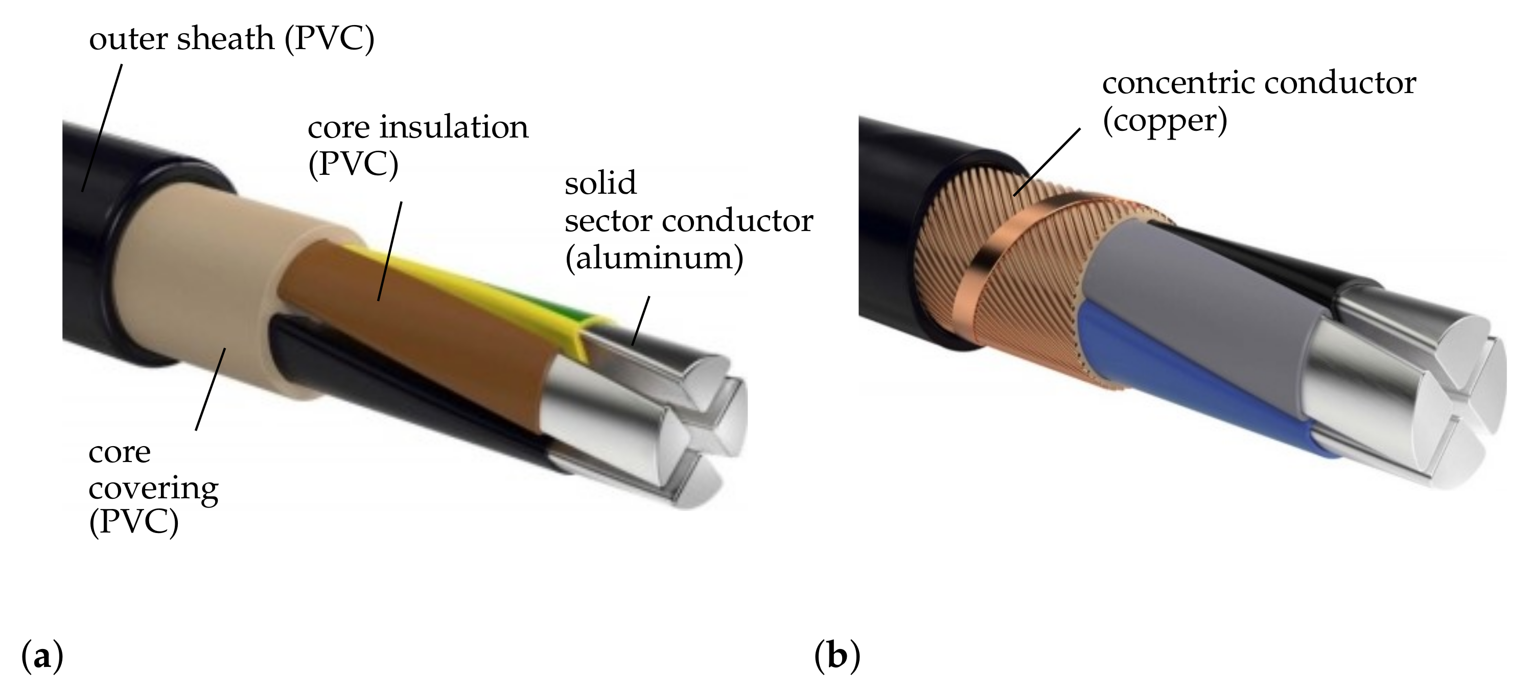
Figure 7.
Conceptual sketch of derived line model (line section of length l, mutual inductances, and capacitances incomplete).
Figure 7.
Conceptual sketch of derived line model (line section of length l, mutual inductances, and capacitances incomplete).

Figure 8.
NAYCWY 4 × 50 SE/25 test cable (sheath cut open).

Figure 9.
Ideal cable designs (corresponding test cables).

Figure 10.
Sectional view and parameter definition of a four-core underground cable based on References [26,37].

Figure 11.
Sector-shaped conductors as ideal quarter circles in four-core NAYCWY cable.

Figure 12.
Test setup for measuring resistances and inductances.

Figure 13.
Calculated and measured resistances at (NAYY-J 4150 SE, cable A).

Figure 14.
Measured resistances at different temperatures (NAYY-J 4150 SE, cable A).

Figure 15.
Comparison of calculated and measured mutual inductances.

Figure 16.
Measured self inductances (NAYY-J 4150 SE, cable A).

Figure 17.
A grounding system’s impedance triangle, based on Reference [41].
Figure 17.
A grounding system’s impedance triangle, based on Reference [41].

Figure 18.
Sketch of test feeder

Figure 19.
Voltages at node 19 for different model modifications.

Figure 20.
Voltages at node 19 for configurations K0–K4.

Figure 21.
Active and reactive phase loads.

Figure 22.
Comparison of measured and simulated phase voltages.

Table 1.
Current measurements of different feeders at exemplary LV substations.
| Sub- Station | Feeder (#) | Line Type | Cabinets (∑) | Customers (∑) | Grid Type | ||||
|---|---|---|---|---|---|---|---|---|---|
| A | 1 | Cable/OL | 2 | 22 | Res. | 23.3 A | 5.43 A | 0.23 | 0.24 |
| 2 | Cable | 2 | 10 | Res. | 6.2 A | 1.19 A | 0.19 | 0.19 | |
| B | 1 | Cable | 1 | 7 | Res. | 5.6 A | 1.11 A | 0.20 | 0.30 |
| C | 1 | Cable | 1 | 1 | Ind. | 6.0 A | 3.24 A | 0.54 | 0.63 |
| 2 | Cable | 1 | 4 | Ind. | 6.9 A | 1.83 A | 0.26 | 0.29 | |
| D | 1 | Cable/OL | 0 | 8 | Res. | 8.7 A | 0.54 A | 0.06 | 0.07 |
| 2 | Cable | 1 | 14 | Res. | 16.3 A | 6.53 A | 0.40 | 0.42 | |
| 3 | Cable | 0 | 14 | Res. | 6.8 A | 2.49 A | 0.37 | 0.52 | |
| 4 | Cable | 1 | 21 | Res. | 13.4 A | 8.83 A | 0.66 | 0.93 | |
| 5 | Cable | 1 | 19 | Res. | 15.5 A | 6.18 A | 0.40 | 0.46 | |
| 6 | OL | 0 | 8 | Res. | 6.0 A | 0.94 A | 0.16 | 0.15 | |
| E | 1 | Cable/OL | 0 | 13 | Res. | 9.5 A | 2.93 A | 0.31 | 0.35 |
| 2 | Cable | 0 | 9 | Res. | 3.6 A | 0.95 A | 0.26 | 0.35 | |
| 3 | Cable/OL | 0 | 8 | Res. | 15.8 A | 1.90 A | 0.12 | 0.12 | |
| 4 | Cable | 0 | 3 | Res. | 2.4 A | 0.67 A | 0.27 | 0.26 | |
| F | 1 | Cable | 0 | 1 | Hotel | 9.5 A | 1.29 A | 0.14 | 0.19 |
| G | 1 | OL | 0 | 7 | Res. | 13.2 A | 0.77 A | 0.06 | 0.06 |
| 2 | OL | 0 | 3 | Res. | 5.7 A | 0.54 A | 0.10 | 0.10 |
Table 2.
Time dependency of current measurements at substation A, feeder 2.
| Time | ||||
|---|---|---|---|---|
| 11:23 a.m. | 6.91 A | 1.13 A | 0.16 | 0.16 |
| 11:25 a.m. | 2.24 A | 0.42 A | 0.19 | 0.19 |
| 11:39 a.m. | 2.37 A | 0.47 A | 0.20 | 0.17 |
| 12:40 p.m. | 6.24 A | 1.19 A | 0.19 | 0.19 |
| 12:43 p.m. | 3.57 A | 0.72 A | 0.20 | 0.21 |
| 12:45 p.m. | 5.59 A | 1.05 A | 0.19 | 0.21 |
| Mean | 4.49 A | 0.83 A | 0.19 | 0.19 |
| RSD | 0.45 | 0.41 | 0.08 | 0.11 |
Table 3.
Measurements at PEN busbars of different substations.
| Sub- Station | Feeders (∑) | Customers (∑) | |||||
|---|---|---|---|---|---|---|---|
| B | 10 | 111 | 34.62 A | 34.41 A | 1.62 A | 0.05 | 0.04 |
| C | 6 | 12 | 27.41 A | 26.17 A | 1.39 A | 0.05 | 0.06 |
| D | 6 | 84 | 57.00 A | 54.01 A | 4.28 A | 0.08 | 0.07 |
| E | 6 | 48 | 52.52 A | 51.50 A | 1.05 A | 0.02 | 0.02 |
| F | 8 | 19 | 37.32 A | 37.20 A | 0.47 A | 0.01 | 0.00 |
| G | 2 | 10 | 8.39 A | 8.10 A | 0.46 A | 0.06 | 0.05 |
| H | 2 | 9 | 5.80 A | 5.10 A | 1.09 A | 0.21 | 0.20 |
| Soil Type | in m (Mean Value) |
|---|---|
| Marshy soil | 30 |
| Clay or humus soil, arable land | 100 |
| Sandy soil (humid) | 200 |
| Sandy soil (dry) | 1100 |
| Stony soil | 1000 |
| Concrete (1 part of cement, 3 parts of sand) | 150 |
| Aluminum ( 20 ) | |
| Stainless steel strip for foundation grounding | ≤ |
Table 5.
Test cables for measurements.
| Cable Type | Manufacturer | Length | |
|---|---|---|---|
| A | NAYY-J 4150 | Bayka [30] | ≈ |
| B | NAYY-J 450 | Bayka [30] | ≈ |
| C | NAYCWY 450 SE/25 | Bayka [31] | ≈ |
| D | NAYCWY 350 SE/50 | Faber [32] | ≈ |
Table 6.
Evaluation of skin and proximity effect factors for and , approximated for aluminum sector conductors.
Table 6.
Evaluation of skin and proximity effect factors for and , approximated for aluminum sector conductors.
| x | ||||||
|---|---|---|---|---|---|---|
| 0 | 50 | 0.16 | 1.0002 | 1.0004 | 1.0006 | |
| 150 | 0.28 | 1.0021 | 1.0054 | 1.0075 | ||
| 20 | 50 | 0.16 | 1.0002 | 1.0003 | 1.0005 | |
| 150 | 0.27 | 1.0018 | 1.0036 | 1.0053 | ||
| 70 | 50 | 0.14 | 1.0001 | 1.0002 | 1.0003 | |
| 150 | 0.25 | 1.0012 | 1.0025 | 1.0037 |
Table 7.
Measured capacitances in at 50 and – 24 .
| Cable Type | ||||
|---|---|---|---|---|
| A | NAYY-J 4150 | 0.17 | 0.01 | – |
| B | NAYY-J 450 | 0.13 | 0.01 | – |
| C | NAYCWY 450 SE/25 | 0.11 | 0.01 | 0.22 |
| D | NAYCWY 3 50 SE/50 | 0.09–0.10 | – | 0.35 |
Table 8.
Comparison of two different methods to approximate of a foundation grounding device.
| Reference | Formula | Approximation Based on | Result | |
|---|---|---|---|---|
| [43] | Hemispherical grounding electrode | |||
| [41] | Soil-embedded circular ring electrode |
Table 9.
Allocation of loads to costumer nodes and phases (Base scenario K0).
| Node | Base Load | PV Plant | EV |
|---|---|---|---|
| PQ Load | PQ Load | PQ Load | |
| P = + 100 W | P = − 4600 W | P = + 4600 W | |
| (ind.) | |||
| 10 | a, b, c | – | – |
| 11 | a, b, c | b | – |
| 12 | a, b, c | a | – |
| 13 | a, b, c | b | – |
| 14 | a, b, c | – | – |
| 15 | a, b, c | a | – |
| 16 | a, b, c | – | – |
| 17 | a, b, c | a | – |
| 18 | a, b, c | – | – |
| 19 | a, b, c | a | c |
Table 10.
Configurations for distribution of load groups to connection phases.
| K0 | K1 | K2 | K3 | |
|---|---|---|---|---|
| a | 4PV | 4PV | 2PV | 1EV |
| b | 1EV | 2PV | 4PV | 4PV |
| c | 2PV | 1EV | 1EV | 2PV |
Publisher’s Note: MDPI stays neutral with regard to jurisdictional claims in published maps and institutional affiliations. |
© 2021 by the authors. Licensee MDPI, Basel, Switzerland. This article is an open access article distributed under the terms and conditions of the Creative Commons Attribution (CC BY) license (http://creativecommons.org/licenses/by/4.0/).
Share and Cite
MDPI and ACS Style
Geis-Schroer, J.; Hubschneider, S.; Held, L.; Gielnik, F.; Armbruster, M.; Suriyah, M.; Leibfried, T. Modeling of German Low Voltage Cables with Ground Return Path. Energies 2021, 14, 1265. https://doi.org/10.3390/en14051265
AMA Style
Geis-Schroer J, Hubschneider S, Held L, Gielnik F, Armbruster M, Suriyah M, Leibfried T. Modeling of German Low Voltage Cables with Ground Return Path. Energies. 2021; 14(5):1265. https://doi.org/10.3390/en14051265
Chicago/Turabian StyleGeis-Schroer, Johanna, Sebastian Hubschneider, Lukas Held, Frederik Gielnik, Michael Armbruster, Michael Suriyah, and Thomas Leibfried. 2021. "Modeling of German Low Voltage Cables with Ground Return Path" Energies 14, no. 5: 1265. https://doi.org/10.3390/en14051265
Note that from the first issue of 2016, this journal uses article numbers instead of page numbers. See further details here.