


1. Introduction
Self-sustained oscillations can be observed in many natural phenomena, such as oscillatory chemical reactions (Kuramoto Reference Kuramoto1984), spiking neurons (Ermentrout & Terman Reference Ermentrout and Terman2010), cardiac cells (Kojima, Kaneko & Yasuda Reference Kojima, Kaneko and Yasuda2006) and vortex shedding (Zdravkovich Reference Zdravkovich1996). Such systems can be interpreted as limit-cycle oscillators. One interesting phenomenon observed in oscillating dynamics is synchronization (Kuramoto Reference Kuramoto1984; Pikovsky, Rosenblum & Kurths Reference Pikovsky, Rosenblum and Kurths2001; Ermentrout & Terman Reference Ermentrout and Terman2010). Although such dynamical systems are generally nonlinear and can be infinite-dimensional, their periodic nature allows the dynamics to be represented in a simplified manner using phase-reduction theory, which is a powerful tool that allows synchronization characteristics to be analysed by considering only the phase dynamics of the system (Kuramoto Reference Kuramoto1984; Pikovsky et al. Reference Pikovsky, Rosenblum and Kurths2001; Ermentrout & Terman Reference Ermentrout and Terman2010; Nakao Reference Nakao2016).
Phase-reduction theory has been extended for many different kinds of oscillatory dynamics such as in time-delayed systems and hybrid systems (Kotani et al. Reference Kotani, Yamaguchi, Ogawa, Jimbo, Nakao and Ermentrout2012; Novičenko & Pyragas Reference Novičenko and Pyragas2012; Shirasaka, Kurebayashi & Nakao Reference Shirasaka, Kurebayashi and Nakao2017). In the field of fluid mechanics, recent work by Kawamura & Nakao (Reference Kawamura and Nakao2013, Reference Kawamura and Nakao2015) considers the extension of phase-reduction theory for periodic spatiotemporal patterns to analyse Hele-Shaw flows. More recently, a computational study for the lock-on of vortex shedding to oscillatory actuation was considered in the work of Taira & Nakao (Reference Taira and Nakao2018) and Khodkar & Taira (Reference Khodkar and Taira2020).
In cases where the oscillating fluid flow comes into contact with an elastic structure, the dynamics need to be considered as a problem of fluid–structure interaction (FSI). The surrounding structure displacement will cause movement of the fluid boundaries. Conversely, the fluid flow exerts force on the fluid–structure interface, causing structural displacements (Richter Reference Richter2017). A common example of an oscillatory phenomenon involving FSI is a vibrating flexible structure within vortex shedding (Gomes & Lienhart Reference Gomes and Lienhart2013). Self-oscillation induced by FSI is also observed in the study of micro-electromechanical systems (Ducloux et al. Reference Ducloux, Talbi, Gimeno, Viard, Pernod, Preobrazhensky and Merlen2007). In biological systems, it is known that the efferent activity of the sympathetic nervous system on vascular smooth muscle alters the contractility of blood vessels, which in turn modulates the periodic blood flow (Kotani et al. Reference Kotani, Struzik, Takamasu, Stanley and Yamamoto2005; Shiogai, Stefanovska & McClintock Reference Shiogai, Stefanovska and McClintock2010). Theoretical formulation using phase-reduction for elastohydrodynamic synchronization of beating flagella has been considered in the work of Kawamura & Tsubaki (Reference Kawamura and Tsubaki2018). However, much remains unknown about oscillation and synchronization in fluid–structure coupled dynamics.
In this work, we present the utilization of phase-reduction for FSI dynamics as the first step to understand how oscillatory flow can be regulated by weak perturbation on the surrounding structure. We describe the model problem of vortex shedding past a cylinder within an elastic structure as well as the phase-reduction theory in § 2. The dependence of the phase-response property on the material types and the location of the perturbation as well as the synchronization characteristics are discussed in § 3. Finally, concluding remarks are given in § 4. The method presented here can be seen as a simplified yet powerful approach to analyse a complex dynamical system involving multiphysics, such as FSI, by reducing it into single scalar phase dynamics.
2. Methods
2.1. Model definition
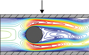
In this study, we define a model of two-dimensional laminar incompressible flow past a cylinder within a channel surrounded by an elastic structure, as shown in figure 1. The cylinder itself is considered as a static rigid body with diameter  $d=0.1\ \textrm {m}$ centred at
  $(x,y)=(0.2\ \text {m}, 0.1\ \text {m})$. The fluid and structure are fully coupled (Horn & Turek Reference Horn and Turek2006; Richter Reference Richter2017). Numerical simulations are conducted based on the finite element method using COMSOL Multiphysics 5.5.

Figure 1. The model used in this study. The elastic structure domain surrounding the fluid domain is marked by the hatched pattern. The cylinder is centred at  $(x,y)=(0.2\ \textrm {m},0.1\ \textrm {m})$.
The fluid flow is governed by the incompressible Navier–Stokes equations in the arbitrary Lagrangian–Eulerian (ALE) formulation (Quarteroni, Tuveri & Veneziani Reference Quarteroni, Tuveri and Veneziani2000; Horn & Turek Reference Horn and Turek2006) such that
 \begin{align} \rho_f \left\{ \dfrac{\partial\boldsymbol{u}_f}{\partial t} + [(\boldsymbol{u}_f - \boldsymbol{u}_m) \boldsymbol{\cdot} \boldsymbol{\nabla}] \boldsymbol{u}_f \right\} = \boldsymbol{\nabla} \boldsymbol{\cdot} \left\{-p {\boldsymbol{\mathsf{I}}} + \mu \left[\boldsymbol{\nabla} \boldsymbol{u}_f + (\boldsymbol{\nabla} \boldsymbol{u}_f)^\text{T}\right]\right\} \quad \text{and} \quad \boldsymbol{\nabla} \boldsymbol{\cdot} \boldsymbol{u}_f = 0, \end{align}
where  $\rho _f$,
  $\mu$,
  $p$,
$p$,  $\boldsymbol {u}_f$,
  $\boldsymbol {u}_m$ and
  ${\boldsymbol{\mathsf{I}}}$ represent fluid density, dynamic viscosity, pressure, fluid flow velocity, spatial coordinate velocity and identity matrix. The external volume forces are assumed to be zero. The fluid flows inside the channel from left to right. The outlet is prescribed with zero-pressure boundary condition. A no-slip boundary condition is prescribed at the fluid–structure interface and around the cylinder wall. A parabolic velocity profile is prescribed at the inlet such that
  $\boldsymbol {u}(0,y) = \bar {U}_{f}{6y(H-y)}/{H^2}$, where
  $\bar {U}_{f}$ is the mean inlet velocity and
  $H=0.2\ \textrm {m}$ is the channel width.
The surrounding structure is modelled as an isotropic linear elastic material. The dynamics is governed by
 \begin{equation} \rho_s \left( \dfrac{\partial^2\boldsymbol{w}_s}{\partial t^2} + \alpha \dfrac{\partial\boldsymbol{w}_s}{\partial t} \right) = \boldsymbol{\nabla} \boldsymbol{\cdot} \left( {\boldsymbol{\mathsf{P}}}^\text{T} + \beta \dfrac{\partial {\boldsymbol{\mathsf{P}}}^\text{T}}{\partial t} \right) + \varepsilon \boldsymbol{\eta}_s (\boldsymbol{x},t), \end{equation}
where  $\rho _s$,
  $\boldsymbol {w}_s$,
  $\alpha$,
  $\beta$ and
  ${\boldsymbol{\mathsf{P}}}$ represent structure density, displacement, mass damping coefficient, stiffness damping coefficient and the first Piola–Kirchoff stress tensor (Formato et al. Reference Formato, Romano, Formato, Sorvari, Koiranen, Pellegrino and Villeco2019). The stress tensor
  ${\boldsymbol{\mathsf{P}}}$ is characterized by Young's modulus
  $E$ and Poisson's ratio
  $\nu$ of the structure material according to Hooke's law. In this work, we define
  $\alpha =0.2\ \textrm {s}^{-1}$ and
  $\beta =0.1\ \textrm {s}$. The width of the elastic structure is set at 0.02 m for both the top and bottom sides. Zero displacement is prescribed at the left and right edges of the structure. The perturbation
  $\varepsilon \boldsymbol {\eta }_s (\boldsymbol {x},t)$ is defined as a localized force at the upper boundary of the structure, as shown in figure 1, such that
 \begin{align} \varepsilon \boldsymbol{\eta}_s (\boldsymbol{x},t) = -\varepsilon \delta \left(\boldsymbol{x}-\boldsymbol{x}_0 \right) \eta(t) \hat{\boldsymbol{e}}_y \quad \text{and} \quad \delta \left(\boldsymbol{x}-\boldsymbol{x}_0 \right) = \dfrac{1}{\sqrt{2{\rm \pi}}\sigma_x} \exp \left[ -\dfrac{1}{2} \left( \dfrac{\boldsymbol{x}-\boldsymbol{x}_0}{\sigma_x} \right)^2 \right] , \end{align}
where  $\boldsymbol {x}$ is the spatial coordinate,
  $\delta (\boldsymbol {x}-\boldsymbol {x}_0 )$ describes the spatial impulse profile and
  $\hat {\boldsymbol {e}}_y$ is the unit vector in the
  $y$ direction, while the negative sign signifies that the perturbation is applied in the direction into the structure domain. The time-varying component
  $\eta (t)$ is defined as
 \begin{equation} \eta(t) = \begin{cases} \dfrac{1}{\sqrt{2{\rm \pi}}\sigma_t} \exp \left[ -\dfrac{1}{2} \left( \dfrac{t-t_0}{\sigma_t} \right)^2 \right], & \text{for impulse perturbation},\\ \sin(\omega_f t), & \text{for sinusoidal perturbation}. \end{cases} \end{equation}
Both the spatial and temporal impulse profiles are approximated as Gaussian functions with  $\sigma _x=0.01\ \textrm {m}$ and
  $\sigma _t=0.01\ \textrm {s}$. We use the impulse perturbation to evaluate the phase-sensitivity function of the oscillating flow, which is necessary in the phase-reduction analysis, and the sinusoidal perturbation to evaluate synchronization of the oscillating flow (more later in § 2.2). The perturbation amplitudes are chosen such that
  $\varepsilon =0.001\ \textrm {N}$ for the case of impulse perturbation and
  $\varepsilon \in [0,25]\ \textrm {N}$ for the case of periodic perturbation.
The kinematic and dynamic coupling conditions are satisfied at the fluid–structure interface  $\varOmega$ (Richter Reference Richter2017), that is,
 \begin{equation} \boldsymbol{u}_f \bigg|_\varOmega = \boldsymbol{u}_s \bigg|_\varOmega = \dfrac{\partial \boldsymbol{w}_s}{\partial t} \bigg|_\varOmega \quad \text{and} \quad \boldsymbol{F}_n \bigg|_\varOmega = \hat{\boldsymbol{e}}_n \boldsymbol{\cdot} \{-p{\boldsymbol{\mathsf{I}}} + \mu [\boldsymbol{\nabla} \boldsymbol{u}_f + (\boldsymbol{\nabla} \boldsymbol{u}_f)^\text{T}]\} \bigg|_\varOmega, \end{equation}
where  $\boldsymbol {u}_s$ is the velocity of the structure displacement,
  $\boldsymbol {F}_n$ is the normal force per unit area exerted on the structure by the fluid and
  $\hat {\boldsymbol {e}}_n$ is a unit vector normal to the fluid–structure interface.
We characterize the model problem by the cylinder-diameter-based Reynolds number  $Re$, Cauchy number
  $C_Y$ and fluid-to-structure density ratio
  $\mathcal {M}$ (DeNayer et al. Reference DeNayer, Apostolatos, Wood, Bletzinger, Wüchner and Breuer2018), which are defined as
 \begin{equation} Re=\dfrac{\rho_f \bar{U}_f d}{\mu}, \quad C_Y=\dfrac{\rho_f \bar{U}_f^2}{E} \quad \text{and} \quad \mathcal{M}=\dfrac{\rho_f}{\rho_s}. \end{equation}
 Table 1 shows the material properties that are considered in this study. Using properties of material type 1, but by modifying the value of  $\mu$, it is found that limit-cycle oscillation occurs for
  $90 \le Re \le 300$. For all material types defined, the fluid properties are chosen such that
  $Re=100$. Material type 1 is used as base values for comparisons. For types 2 and 3, the value of
  $C_Y$ is modified by changing
  $E$ with a ratio of 1.25 times the base value. For types 4 and 5, the value of
  $\mathcal {M}$ is modified by changing
  $\rho _s$ with a ratio of 1.25 times the base value. For types 6 and 7,
  $\nu$ is modified with a ratio of 1.2 times the base value to keep it within the range for an isotropic linear elastic material (
 $-1.0 < \nu < 0.5$). For type 8, both fluid and structure properties are changed while keeping the values of
  $Re$,
$Re$,  $C_Y$,
  $\mathcal {M}$ and
  $\nu$ equal to the base values.
Table 1. The types of fluid and structure material properties considered in this study.

The computational domain is discretized using a distributed quadrilateral mesh with a total number of 2864 elements. The elements around the cylinder and the fluid–structure interface are more refined with maximum size limit at  $6.72 \times 10^{-3}\ \textrm {m}$ and minimum size limit at
  $9.6 \times 10^{-5}\ \textrm {m}$. Implicit time stepping is used and the simulation output is stored every
  $\Delta t = 0.0005\ \textrm {s}$.
2.2. Phase-reduction
Here, we briefly describe the phase-reduction theory and its use for analysing synchronization characteristics (Nakao Reference Nakao2016; Taira & Nakao Reference Taira and Nakao2018). Let us write the governing dynamics of an oscillating FSI dynamics that is perturbed by an external force as
 \begin{equation} \dfrac{\partial}{\partial t}\boldsymbol{X}(\boldsymbol{x},t)=\boldsymbol{F}\{\boldsymbol{X}\} + \varepsilon \boldsymbol{\eta}(\boldsymbol{x},t), \end{equation}
where  $\boldsymbol {X} = [\boldsymbol {u}_f, \boldsymbol {w}_s]$ is the system state,
  $\boldsymbol {F}\{\boldsymbol {X}\}$ is the system dynamics and the perturbation
  $\varepsilon \boldsymbol {\eta }(\boldsymbol {x}, t)$ is sufficiently small. We assume that the system has an exponentially stable limit-cycle solution
  $\boldsymbol {X}_0$ with frequency
  $\omega _n$, such that
  $\boldsymbol {X}_0(\boldsymbol {x}, t+2{\rm \pi} /\omega _n) = \boldsymbol {X}_0(\boldsymbol {x}, t)$ is satisfied. A phase functional
  $\varTheta [\boldsymbol {X}]$ that maps the system state to a scalar phase value
  $\theta \in [0,2{\rm \pi} )$ can be introduced (Nakao, Yanagita & Kawamura Reference Nakao, Yanagita and Kawamura2014), such that the phase of the system
  $\theta = \varTheta [\boldsymbol {X}]$ always increases with a constant frequency as
  $\dot {\theta }(t) = \int ( \delta \varTheta / \delta \boldsymbol {X} ) \boldsymbol {\cdot } \boldsymbol {F}\{ \boldsymbol {X} \} \,\textrm {d}\boldsymbol {x} = \omega _n$ in the basin of the limit cycle when the perturbation is absent, where
  $\delta \varTheta / \delta \boldsymbol {X}$ is the functional derivative of
  $\varTheta [\boldsymbol {X}]$ at
  $\boldsymbol {X} = \boldsymbol {X}(\boldsymbol {x}, t)$. At the lowest-order approximation (neglecting the higher-order-terms),
  $\delta \varTheta / \delta \boldsymbol {X}$ can be approximately evaluated at
  $\boldsymbol {X} = \boldsymbol {X}_0(\boldsymbol {x}, \theta / \omega _n)$ on the limit cycle and the phase dynamics under weak perturbation can be found as
 \begin{equation} \dot{\theta}(t) = \omega_n + \varepsilon \int \boldsymbol{Z}(\boldsymbol{x}, \theta) \boldsymbol{\cdot} \boldsymbol{\eta}(\boldsymbol{x}, t)\,\textrm{d}\boldsymbol{x}, \end{equation}
where  $\boldsymbol {Z}(\boldsymbol {x}, \theta ) = [\boldsymbol {Z}_{f}(\boldsymbol {x}, \theta ), \boldsymbol {Z}_{s}(\boldsymbol {x}, \theta )] = \delta \varTheta / \delta \boldsymbol {X}|_{\boldsymbol {X} = \boldsymbol {X}_0(\boldsymbol {x}, \theta /\omega _n)}$ is known as the phase-sensitivity function. If
  $\boldsymbol {Z}(\boldsymbol {x}, \theta )$ is known, the influence of any perturbation function
  $\varepsilon \boldsymbol {\eta }(\boldsymbol {x}, t)$ can be determined through (2.8). In particular, if the perturbation on the structure is spatially localized in the form
  $\boldsymbol {\eta }(\boldsymbol {x}, t) = [\boldsymbol {\eta }_f(\boldsymbol {x},t),\boldsymbol {\eta }_s(\boldsymbol {x},t)] = [0,-\delta (\boldsymbol {x} - \boldsymbol {x}_0) \eta (t) \hat {\boldsymbol {e}}_y]$, the phase equation reads as
  $\dot {\theta }(t) = \omega _n + \varepsilon Z_y(\theta ) \eta (t)$, where
  $Z_y(\theta ) =\int \boldsymbol {Z}_{s}(\boldsymbol {x}_0, \theta ) \boldsymbol {\cdot } [-\delta (\boldsymbol {x}-$
  $ \boldsymbol {x}_0) \hat {\boldsymbol {e}}_y]\,\textrm {d}\boldsymbol {x}$.
In this work, we evaluate  $Z_y(\theta )$ using the direct impulse perturbation approach (Ermentrout & Terman Reference Ermentrout and Terman2010; Nakao Reference Nakao2016), with the perturbation function
  $\varepsilon \boldsymbol {\eta }_s (\boldsymbol {x}, t)$ defined in (2.3a,b) and (2.4). By introducing the impulse at certain phase
  $\theta$ (determined by
  $t_0$), the phase dynamics will be affected, where phase shift will be observed along the limit-cycle orbit. This asymptotic phase shift is known as the phase-response function
  $g(\theta;\varepsilon \hat {\boldsymbol {e}}_y)$, which is dependent on the amplitude, location, direction and phase where it is introduced. Hence, the phase-sensitivity function at phase
  $\theta$ can be evaluated as
 \begin{equation} Z_y(\theta) = \lim_{\varepsilon \to 0} \dfrac{g(\theta;\varepsilon \hat{\boldsymbol{e}}_y)}{\varepsilon} \approx \dfrac{g(\theta;\varepsilon \hat{\boldsymbol{e}}_y)}{\varepsilon}. \end{equation}
Therefore, we can evaluate  $Z_y(\theta )$ by introducing impulse perturbations over the entire range of
  $\theta$. By evaluating
  $g(\theta;\varepsilon \hat {\boldsymbol {e}}_y)$ using appropriate observables showing periodic oscillations,
  $Z_y(\theta )$ can be determined using a limited number of measurements. In this study, we consider the oscillating lift coefficient
  $C_L$ on the cylinder boundaries as the observable. The relative phase value of
  $\theta =\{0,2{\rm \pi} \}$ is defined at the minimum value of
  $C_L$ oscillation.
The representation in phase dynamics allows further analysis to determine the conditions in which the original dynamics will synchronize to a periodic perturbation with period  $T_f$ and frequency
  $\omega _f=2{\rm \pi} /T_f$. We consider the phase difference
  $\phi (t)$ between the phase of the original oscillatory dynamics
  $\theta (t)$ and the periodic perturbation
  $\omega _f t$ such that
 \begin{equation} \phi(t) \equiv \theta(t)-\omega_f t. \end{equation}
Combining with (2.8) for the case where a perturbation is applied on the structure and by applying the averaging approximation (Ermentrout & Terman Reference Ermentrout and Terman2010), we can evaluate the rate of change of  $\phi (t)$ such that
 \begin{align} \dot{\phi}(t) = \omega_n-\omega_f + \varepsilon \varGamma(\phi) \quad \text{and} \quad \varGamma(\phi) = \dfrac{1}{2{\rm \pi}}\int_{0}^{2{\rm \pi}}Z_y(\phi + \psi) \boldsymbol{\cdot} \eta(\psi/\omega_f)\,\textrm{d}\psi, \end{align}
where  $\varGamma (\phi )$ is known as the phase-coupling function, which is
  $2{\rm \pi}$-periodic, and
  $\psi =\omega _f t$.
By conducting stability analysis on the phase dynamics in (2.11a), we can determine the criteria for which the original oscillating dynamics will synchronize to a periodic perturbation, that is, when  $\vert \dot {\phi }\vert \to 0$ and
  $\omega _n$ converges to
  $\omega _f$. In this case, the original limit-cycle oscillation exhibits phase-locking to the periodic perturbation asymptotically at a stable fixed point
  $\phi$. Through observation of (2.11a), we can find that the phase dynamics stability is satisfied if
 \begin{equation} \varepsilon\min{\varGamma(\phi)} < \omega_f -\omega_n < \varepsilon\max{\varGamma(\phi)}. \end{equation}
Using this stability criterion, we can determine the boundaries of the synchronization region over the  $(\omega _f/\omega _n)$–
 $\varepsilon$ space. These synchronization boundaries are also known as the Arnold tongue (Pikovsky et al. Reference Pikovsky, Rosenblum and Kurths2001) and will be discussed later in § 3.
On the contrary, periodic phase slip will occur if  $\vert \dot {\phi }\vert > 0$ and the phase difference
  $\phi (t)$ will continuously increase over time (Nakao Reference Nakao2016). We can define the frequency of this periodic phase slip as
  $f_{slip} = 1/T_{slip}$, where
  $T_{slip}$ is the interval of the periodic phase slip, which is calculated as a function of frequency difference
  $\omega _n - \omega _f$. When the original oscillating dynamics is phase-locked to the periodic perturbation, the mean frequency of the oscillation is equal to
  $\omega _f$ and
  $f_{slip} \approx 0$. Outside of the phase-locking region, phase slip will occur and
  $f_{slip}$ can be calculated as
 \begin{equation} f_{slip}=\dfrac{1}{T_{slip}} \quad \text{and} \quad T_{slip}=\int_{0}^{2{\rm \pi}} \dfrac{\textrm{d}\phi}{\omega_n-\omega_f + \varepsilon \varGamma(\phi)}. \end{equation}
Depending on the frequency difference, the approximated value of  $f_{slip}$ can be positive or negative. The characteristics of the
  $f_{slip}$ curve over the span of
  $\omega _n - \omega _f$ can be compared with the results from actual direct numerical simulations (DNS), as seen later in § 3.
3. Results and discussion
3.1. Phase-sensitivity analysis
In what follows, we compare the phase-sensitivity function  $Z_y(\theta )$ for different material types, given that the impulse perturbation defined in (2.3a,b) and (2.4) is introduced. The findings in this section can be further utilized to evaluate the phase-coupling function and to analyse the synchronization characteristics. For each material type, 11 actual simulations were performed at equal phase intervals over
  $\theta$ (shown by markers in figures 2 and 3) and the in-between values are obtained by the modified Akima interpolation method using MATLAB.

Figure 2. ( $a$) Periodic
  $C_L$ oscillation for material types 1 and 8. (
 $b$) Comparison of
  $Z_y(\theta )$ for different perturbation locations. The solid and dotted lines show the results for material types 1 and 8, respectively.

Figure 3. (a) Comparison of  $Z_y(\theta )$ for different values of
  $C_Y$ (shown in units of
  $1 \times 10^{-8}$). (b) Comparison of
  $Z_y(\theta )$ for different values of
  $\mathcal {M}$. (c) Comparison of
  $Z_y(\theta )$ for different values of
  $\nu$.
Figure 2(a) shows a comparison of the  $C_L$ oscillations between material types 1 and 8 in which both the fluid and structure properties are changed but all the characteristic numbers are kept equal. The period of the
  $C_L$ oscillations is found at
  $T_n=0.403$ s for material types 1 to 7, while for material type 8 the period is found at
  $T_n=0.323$ s, showing that the oscillation is mainly characterized by the fluid properties (see table 1). For all material types, the vortex shedding frequency is 3.5 times or more higher than the dominant harmonic frequency of the structure, such that large structural resonance due to the vortex shedding does not occur. Note that in the present study damping terms are included in the structural dynamics, such that the structure harmonic modes have negligible effect on the limit-cycle oscillation as time goes to infinity.
We confirm that the chosen characteristic numbers used in this study determine the phase dynamics by the results shown in figure 2(b), where close agreement can be seen between  $Z_y(\theta )$ evaluated for material types 1 and 8 (shown as solid and dotted lines, respectively). As shown in figure 2(a), the
  $C_L$ oscillation periods for material types 1 and 8 differ due to the different mean inlet velocities. Nevertheless, when all the values of
  $Re$,
$Re$,  $C_Y$,
  $\mathcal {M}$ and
  $\nu$ are matched (see table 1), the obtained phase-sensitivity functions are in close agreement. This shows that for an equal model configuration, the phase dynamics is characterized by the values of
  $Re$,
$Re$,  $C_Y$,
  $\mathcal {M}$ and
  $\nu$.
Figure 2(b) also shows that the phase-sensitivity function  $Z_y(\theta )$ is significantly affected by the perturbation location. We compare the results for perturbations applied in between the upstream and downstream sides relative to the cylinder centre on the
  $x$ axis at
  $x=0.2\ \textrm {m}$. Smaller mean and peak-to-peak values are observed for perturbations applied at the upstream side (
 $x_0 < 0.2\ \textrm {m}$) while larger values are observed for the cases where perturbations are applied at the downstream side (
 $x_0 > 0.2\ \textrm {m}$). In the upstream region, flow separation has yet to occur such that the oscillating flow is not fully developed. Hence, for an equal impulse perturbation amplitude, the phase-response is considerably smaller than in the case when the perturbation is applied at the downstream side where vortices are starting to develop. These also suggest that the required periodic perturbation amplitude and frequency to achieve synchronization, as defined in (2.12), are also dependent on the perturbation location, which will be studied in the next subsection.
We further investigate the effect of each characteristic number by comparing the response to impulse perturbation introduced at  $x_0 = 0.25$ m. As mentioned in § 2.1, we modify the Cauchy number
  $C_Y$ and the fluid-to-structure density ratio
  $\mathcal {M}$ by changing the Young's modulus
  $E$ and structure density
  $\rho _s$, respectively. Figure 3(a) shows the comparison for material types 1, 2 and 3, where
  $Z_y(\theta )$ is compared for different values of
  $C_Y$. The mean and peak-to-peak values of
  $Z_y(\theta )$ increase as the value of
  $C_Y$ increases. Figure 3(b) shows the comparison for material types 1, 4 and 5, where
  $Z_y(\theta )$ is compared for different values of
  $\mathcal {M}$. The peak-to-peak value of
  $Z_y(\theta )$ increases as the value of
  $\mathcal {M}$ increases while the mean value is unaffected. Figure 3(c) shows the comparison for material types 1, 6 and 7, where
  $Z_y(\theta )$ is compared for different values of Poisson's ratio
  $\nu$. The mean and peak-to-peak values of
  $Z_y(\theta )$ increase as the value of
  $\nu$ decreases.
Comparisons on the effect of the structure material and fluid–structure coupling characteristic numbers show that the changes in  $\mathcal {M}$ and
  $\nu$ have smaller effects on the phase-sensitivity function than that of
  $C_Y$, even taking into account the narrower range of
  $\nu$ due to the parameter restriction. The change in
  $C_Y$ significantly affects the mean value of the phase-sensitivity function rather than its waveform. Although the effects of
  $C_Y$,
  $\mathcal {M}$ and
  $\nu$ are different, these values characterize the overall phase-response to the perturbation on the elastic structure.
Observation of figures 2 and 3 shows that the impulse perturbation causes phase advancement to the oscillating flow for all the chosen material types and perturbation locations. All the resulting phase-sensitivity functions have positive non-zero mean values. Similar phase-response is typically found in class I neurons (Ermentrout & Terman Reference Ermentrout and Terman2010). These suggest that, if we periodically push the upper boundary of the structure, then the perturbation frequency must be higher than the natural frequency of the oscillating flow in order to achieve synchronization. Such limitation can be avoided if we consider that the perturbation is in the form of a periodic pushing and pulling action on the upper boundary, which is defined in this work as a zero-mean sinusoidal function shown in (2.4).
3.2. Synchronization analysis
We consider material type 1 and the periodic sinusoidal perturbation defined in (2.3a,b) and (2.4) being used for the following synchronization analysis. Given that the phase-sensitivity function  $Z_y(\theta )$ can be determined, we can evaluate the phase-coupling function
  $\varGamma (\phi )$ using (2.11b) for the given perturbation function. The phase-coupling functions evaluated at different perturbation locations
  $x_0$ are shown in figure 4(a). As can be deduced from the peak-to-peak values of
  $Z_y(\theta )$ shown in figure 2(b), the evaluated phase-coupling functions show largest variation over
  $\phi$ when the perturbation is applied at
  $x_0=0.25\ \textrm {m}$. Variation of
  $\varGamma (\phi )$ over negative and positive values suggests that a perturbation frequency lower than the natural frequency of the oscillating flow can also lead to synchronization.

Figure 4. (a) Comparison of the phase-coupling function  $\varGamma (\phi )$ for several perturbation locations. (b) Variation of
  $\varGamma (\phi )$ over the perturbation location. (c) Synchronization boundaries for
  $x_0=0.25\ \textrm {m}$ shown by the solid lines. Results from DNS for synchronizing and non-synchronizing cases are marked with
  $\bigcirc$ and
  $\times$ respectively. (d) Comparison of the
  $f_{slip}$ characteristics calculated by (2.13a,b) for
  $x_0=0.25\ \textrm {m}$ and
  $\varepsilon =10\ \textrm {N}$ with results obtained from DNS, shown by the solid lines and markers, respectively.
Several other numerical simulations for perturbation locations  $x_0 \in [0.1,0.4]\ \textrm {m}$ are conducted to compare their synchronization regions, as shown in figure 4(b). The markers indicate locations where simulations are actually performed. By the criterion for synchronization in (2.12), larger variation of
  $\varGamma (\phi )$ will result in a wider synchronization region. For the given model problem, we found that the widest synchronization region is achieved at
  $0.30 < x_0 < 0.35\ \textrm {m}$. In general, a wider synchronization region is achieved given that the perturbation is applied near the downstream end of the cylinder in which the vortices are fully developed. The synchronization region shrinks as the perturbation location goes farther downstream from the cylinder as the vortices start to decay.
In what follows, we consider the case where periodic perturbation is applied at  $x_0=0.25\ \textrm {m}$. Using the synchronization criterion in (2.12), we can construct a representation of the synchronization region in the form of an Arnold tongue, as shown in figure 4(c). We compare the approximated synchronization region with results obtained from DNS. For the actual simulations, the
  $C_L$ oscillation and the periodic perturbation are considered to be synchronized when their phase difference
  $\phi$ stops growing and exhibits small fluctuations around a certain value (i.e. phase-locking occurs). It can be seen that the approximated synchronization region agrees well with the results from actual simulations of the nonlinear FSI dynamics, especially for smaller values of the perturbation amplitude
  $\varepsilon$. The effect of nonlinearities become more apparent for
  $\varepsilon \ge 15\ \textrm {N}$ in which the actual dynamics starts to deviate from the approximation obtained using phase-reduction theory. As also noted in the work of Taira & Nakao (Reference Taira and Nakao2018), the identification of the Arnold tongue through the phase-coupling function is attractive since we only need to conduct a small number of numerical simulations over the phase
  $\theta \in [0,2{\rm \pi} )$ to determine the synchronization region.
The elastic structure displacement oscillation in the  $y$ direction at
  $x=0.25\ \textrm {m}$ has a mean value of
  $-2.77 \times 10^{-6}\ \textrm {m}$ and a peak-to-peak value of
  $0.54 \times 10^{-6}\ \textrm {m}$ when the periodic perturbation is not applied. For the synchronized case where a periodic perturbation with amplitude
  $\varepsilon =25\ \textrm {N}$ is applied, the displacement has a mean value of
  $-7.97 \times 10^{-6}\ \textrm {m}$ and a peak-to-peak value of 0.004 m. It is also observed that the oscillating displacement in the
  $y$ direction of the elastic structure at the bottom side synchronizes with the periodic perturbation due to the fluid–structure coupling.
We compare the approximated  $f_{slip}$ characteristics evaluated using (2.13a,b) with the results obtained from DNS, as shown in figure 4(d). In this work, the
  $f_{slip}$ characteristic is compared for perturbation amplitude
  $\varepsilon =10\ \textrm {N}$. However, comparisons can be conducted for any value of
  $\varepsilon$. The approximated phase-locking region is shown between the dashed vertical lines. We can see that the
  $f_{slip}$ characteristics obtained from DNS (shown with the markers) is in close agreement with the approximated characteristics obtained from the calculations. However, the actual phase-locking region is slightly biased towards the lower perturbation frequency. This also agrees with the findings seen in figure 4(c) in which the actual synchronization region is biased towards the lower perturbation frequency, especially for larger perturbation amplitudes. These findings further confirm that the linear approximation using phase-reduction captures the synchronization characteristics of the original nonlinear oscillating dynamics.
To the best of our knowledge, this is the first study that uses phase-reduction theory to determine synchronization characteristics of an oscillating flow in FSI dynamics. Here, we have presented the idea of how synchronization between oscillatory flow and periodic forcing on the surrounding elastic structure can be achieved, as well as the use of phase-reduction theory to determine the region of synchronization.
A recent study in the field of microfluidics (Sun et al. Reference Sun, Lin, Rau and Chiu2017) presented a design of microfluidic oscillators where self-sustained flow oscillation induced by impinging jet flow on a bluff body is incorporated for mixing of fluids . It is also known that fluid mixing can be induced by vibration on the wall of the fluid container (Carlsson, Sen & Löfdahl Reference Carlsson, Sen and Löfdahl2005). Combination of these two concepts might reveal an alternative method to enhance the mixing performance, and phase-reduction theory can be applied to estimate the required parameters for obtaining the desired flow regulation, such as presented in this study. The understanding of periodic fluid flow regulation by the motion of an elastic structure is also important for studies of blood pressure regulation due to the movement of vascular branches induced by the activity of the sympathetic nervous system (Kotani et al. Reference Kotani, Struzik, Takamasu, Stanley and Yamamoto2005).
There are, of course, other synchronization cases that can be considered, such as periodic perturbation applied on a structure submerged inside an oscillating fluid flow. In addition, the approach using phase-reduction theory can also be extended to analyse the synchronization around harmonic frequencies. Recent experimental work and mathematical modelling (Barros et al. Reference Barros, Borée, Noack and Spohn2016; Herrmann et al. Reference Herrmann, Oswald, Semaan and Brunton2020) show how symmetric forcing leads to subharmonic synchronization while antisymmetric forcing leads to harmonic synchronization. These phenomena may also be observed in FSI dynamics as well, and phase-reduction theory can also be utilized to uncover synchronization characteristics under symmetric and antisymmetric forcing.
4. Conclusion
We have applied phase-reduction theory to find the synchronization characteristics of vortex shedding by periodic perturbation on the surrounding elastic structure. We have conducted parametric studies to observe how several dimensionless parameters known in FSI dynamics affect the phase dynamics of the limit-cycle oscillation. It is found that the phase-sensitivity function is significantly affected by the Cauchy number, whereas it is affected only rather slightly by the fluid-to-structure density ratio and Poisson's ratio, given that the model configuration and fluid flow characteristic defined by the Reynolds number are equal. The perturbation location on the elastic structure also significantly affects the phase-sensitivity function. Furthermore, it is confirmed that the estimated synchronization characteristics are in close agreement with the results obtained from DNS by comparing the synchronization region and the periodic phase slip characteristics. The synchronization region is maximized given that the sinusoidal perturbation is applied near the downstream end of the cylinder. Our findings open the further possibility for the utilization of phase-reduction theory for synchronization analysis in other practical problems involving oscillations in dynamics governed by fluid–structure interaction, such as in biological systems and control of microfluidics, using only a limited number of experiments or simulations.
Funding
I.A.L. acknowledges the support from the Iwatani Naoji Foundation. K.K. acknowledges the support from the Asahi Glass Foundation and JSPS KAKENHI (grant 18H04122). H.N. acknowledges the support from JSPS KAKENHI (grant JP17H03279) and JST CREST (grant JPMJCR1913).
Declaration of interests
The authors report no conflict of interest.


 Open access