


Abstract
The magma ocean (MO) is a crucial stage in the build-up of terrestrial planets. Its solidification and the accompanying outgassing of volatiles set the conditions for important processes occurring later or even simultaneously, such as solid-state mantle convection and atmospheric escape. To constrain the duration of a global-scale Earth MO, we have built and applied a 1D interior model coupled with either a gray H2O/CO2 atmosphere or with a pure H2O atmosphere treated with a line-by-line model described in a companion paper by Katyal et al. We study in detail the effects of several factors affecting the MO lifetime, such as the initial abundance of H2O and CO2, the convection regime, the viscosity, the mantle melting temperature, and the longwave radiation absorption from the atmosphere. In this specifically multivariable system, we assess the impact of each factor with respect to a reference setting commonly assumed in the literature. We find that the MO stage can last from a few thousand to several million years. By coupling the interior model with the line-by-line atmosphere model, we identify the conditions that determine whether the planet experiences a transient MO or it ceases to cool and maintains a continuous MO. We find a simultaneous dependence of this distinction on the mass of the outgassed H2O atmosphere and on the MO surface melting temperature. We discuss their combined impact on the MO's lifetime in addition to the known dependence on albedo, orbital distance, and stellar luminosity, and we note observational degeneracies that arise thereby for target exoplanets.
Export citation and abstract BibTeX RIS
1. Introduction
The internal thermal structure immediately after terrestrial planets form is not well known. This information is nevertheless important in order to understand the evolution of the atmosphere and the onset and development of mantle convection.
With our numerical model, we simulate the magma ocean (MO) phase, an intermediate stage in thermal evolution between completed accretion and the formation of a young planet's surface. During this period, the duration of which we aim to estimate, a large part of the mantle is fully molten.
Although the existence of the MO on the Moon is a widely accepted hypothesis, due to its primary anorthositic crust (Canup 2004; Sleep et al. 2014; Barboni et al. 2017), such observational evidence remains elusive for Earth. However, the Moon-forming impact is expected to have extensively molten Earth's mantle (e.g., Nakajima & Stevenson 2015). In addition, the release of gravitational potential energy associated with core formation, along with the kinetic energy of accretional impacts and the decay of short-lived radiogenic elements, provides enough energy to globally melt the silicate mantle of an Earth-sized planet, leading to the formation of a MO (Coradini et al. 1983; Solomatov 2007; Elkins-Tanton 2008; Sleep et al. 2014).
During the MO stage, the interior temperature is high, and degassing of volatiles accompanies the thermal evolution (Abe & Matsui 1988; Elkins-Tanton 2008; Schaefer & Fegley 2010; Zahnle et al. 2010; Lebrun et al. 2013; Gaillard & Scaillet 2014; Massol et al. 2016; Salvador et al. 2017). As a result, a secondary atmosphere forms, and it is expected to have provided the bulk of the atmospheric mass during the Hadean. Nevertheless, there is uncertainty in the initial volatile inventory of the Earth because impactors stochastically deliver volatiles to the accreting planets (Morbidelli et al. 2005; Tsiganis et al. 2005; Raymond & Izidoro 2017). The most conservative estimate of the resulting Earth volatile budget considers 300 bar H2O, roughly corresponding to today's ocean, and 100 bar CO2, i.e., the amount estimated to be stored in the crust in the form of carbonates (Ingersoll 2013). However, the existence of abundances in H2O and CO2 higher than those directly observable in the present Earth cannot be excluded and is even likely (Hirschmann & Dasgupta 2009; Hirschmann & Kohlstedt 2012; Hallis et al. 2015). The bulk of the atmosphere outgassed from the MO is suggested to be composed largely of H2O and CO2 for most carbonaceous chondritic materials (Schaefer & Fegley 2010; Lupu et al. 2014) along with reduced species (H, CO, CH4; Gaillard & Scaillet 2014; Lupu et al. 2014), excluding the case of chondritic binary mixtures (Schaefer & Fegley 2017). Proxy evidence for less oxidized early atmosphere is also given by sulfur isotope studies (Ueno et al. 2009; Endo et al. 2016).
As soon as a certain minimum amount of water vapor is present in the atmosphere, its role in planetary evolution is the most crucial of all gases present. This is due to its strong greenhouse effect and the well-studied runaway greenhouse (RG) regime associated with it, which does not allow for radiative equilibrium solutions over a wide range of surface temperatures, while the atmospheric outgoing radiation stalls to a constant value known as the Kombayashi–Ingersoll (KI) or RG limit (e.g., Kasting 1988; Zahnle et al. 1988; Nakajima et al. 1992; Pierrehumbert 2010; Leconte et al. 2013). The RG regime over an MO, however, would occur at surface temperatures in excess of 3000 K that are characteristic of a molten silicate mantle (Lupu et al. 2014; Massol et al. 2016). Previous research has mostly indicated an invariant outgoing radiation limit of ∼300 W m−2 for an Earth-sized planet with a water-dominated atmosphere (Kasting 1988; Zahnle et al. 1988; Nakajima et al. 1992; Zahnle et al. 2007; Kopparapu et al. 2013; Leconte et al. 2013; Hamano et al. 2015; Goldblatt 2015).
In particular, Hamano et al. (2013) extended the gray atmospheric model of Nakajima et al. (1992) to cover high surface temperatures and introduced the separation of the MO stage into short term and long term. Based on their comparison of the stellar irradiation to the KI limit of a H2O-dominated atmosphere, they brought the role of stellar luminosity into the context of the MO lifetime, which, under suitable conditions, can hinder planetary cooling altogether. However, in the Hamano et al. (2013) study, the potential role of mantle composition was not investigated in combination with the explicit role of the surface vapor pressure on the longwave radiation limit. We extend this previous work by considering such factors.
The volatiles that envelop the terrestrial planets are crucial since they quantify the effect of thermal blanketing that delays the radiative cooling of the MO by hundreds of thousands of years. It has been investigated by several authors so far (Abe & Matsui 1988; Elkins-Tanton 2008; Hamano et al. 2013; Lebrun et al. 2013; Hier-Majumder & Hirschmann 2017; Salvador et al. 2017; Ikoma et al. 2018). However, comparing results from the literature is not straightforward because each MO study involves many ad hoc assumptions. This is inevitable because different research fields focus on a specific niche of the MO system. At the same time, the topic is becoming increasingly multidisciplinary (Tasker et al. 2017), and more of the assumptions are being challenged.
Our aim is to calculate the lifetime of the MO and to comprehensively assess the role of various parameters in it. Knowing their relative significance can help guide future model development. Therefore, we primarily account for the key role of the outgassed atmosphere. For planets that are volatile-poor or may quickly lose their atmosphere, blackbody thermal evolution is modeled and discussed. The findings are focused on an Earth-sized rocky planet, yet their applicability in the exoplanetary context is discussed and points of interest for the community are suggested.
2. Methods
2.1. Numerical Model
We calculate the thermal state of the solidifying MO without examining the preceding stage of its formation. We build a model that simulates the coupled evolution of the interior (Sections 2.2–2.7) and the atmosphere (Sections 2.8–2.9). The COnvective Magma Radiative Atmosphere and Degassing (COMRAD) model resolves the mantle interior profiles of temperature and liquid and solid fraction, along with the degassing process, starting from a fully molten mantle up to the end of the MO phase (see Section 2.10). We employ the mantle surface temperature iteration method developed by Lebrun et al. (2013), with differences in the calculation of the mantle adiabat (Section 2.4), of the liquid viscosity (Section 2.6), and of the volatile mass balance (Section 2.7). The outgassing of H2O and CO2 is calculated according to a melt solubility curve for each volatile (Section 2.7). The atmosphere is treated in two alternative ways (Section 2.8): (i) a gray atmosphere accounting for two greenhouse gases, H2O and CO2 (Abe & Matsui 1985; Elkins-Tanton 2008; Section 2.8.1) and (ii) a pure H2O atmosphere with a spectrally resolved Outgoing Longwave Radiation at the Top Of the Atmosphere (henceforth named "OLR at TOA," OLRTOA) by Katyal et al. (2019) in a companion paper (hereafter "companion paper"; Section 2.8.2). In the following sections, we separately introduce each model component.
2.2. Structure of the Interior
We consider a spherically symmetric Earth with outer radius Rp and core radius Rb. This yields a mantle of thickness Rp − Rb, the physical properties of which are defined by the melting curves (solidus and liquidus) of KLB-1 peridotite (Figure 1). By comparing the interior thermal profile to these curves, we identify the phase (liquid, partially molten, or solid) of each mantle layer. The mantle is initially assumed to be fully molten and convecting, with an adiabatic temperature profile. As it cools, the liquid adiabat (dotted line in Figure 1) intersects with the melting curves (solid lines in Figure 1). Due to the steeper slope of the adiabat compared to the melting curves, the adiabat and the liquidus intersect first atop the core–mantle boundary (CMB). The mantle is fully molten from the surface until the depth of intersection between the liquid adiabat and the liquidus, it is partially molten between the liquidus and solidus, and completely solid below the solidus. The melt fraction ϕ at any given depth is calculated as (e.g., Solomatov & Stevenson 1993a, 1993b; Abe 1997; Solomatov 2007; Lebrun et al. 2013)

where T is the temperature of the mantle at a given depth, and Tsol and Tliq the corresponding solidus and liquidus temperatures. The partially molten region is further divided by comparing the melt fraction ϕ with the critical melt fraction ϕC of 40% that separates liquid-like from solid-like behavior (Costa et al. 2009). For ϕ > ϕC, the region is considered liquid-like and belongs to the MO-convecting domain of depth D. Note that ϕC varies among 30% (e.g., Hier-Majumder & Hirschmann 2017; Maurice et al. 2017), 40% (Solomatov 2007; Bower et al. 2017), and 50% (Monteux et al. 2016; Ballmer et al. 2017) in the geodynamic literature.

Figure 1. Melting curves for three cases: linear according to Abe (1997) ("Abe97," purple solid lines); synthetic for peridotitic composition according to Herzberg et al. (2000), Hirschmann (2000), and Zhang & Herzberg (1994) for the upper mantle, and Fiquet et al. (2010) for the lower mantle ("Syn," black solid lines); and chondritic composition according to the same data for the upper mantle and Andrault et al. (2011) for the lower mantle ("Andrault11," yellow solid lines). "Syn" and "Andrault11" differ only in the lower mantle parameterization. The black dashed line indicates the profile of the rheology transition for the "Syn" curves ("RF Syn"). Dotted lines indicate adiabats with potential temperatures of 4000 and 2400 K. The red open and full circles indicate the base of the liquid-like MO of thickness D for the two adiabats, with the corresponding depth ranges of liquid (l), solid (s), and partially molten (l+s) regions shown in the left columns.
Download figure:
Standard image High-resolution image2.3. Melting Curves
We use solidus and liquidus curves of KLB-1 peridotite obtained from experimental data. Depending on pressure, we adopt different parameterizations for different parts of the mantle. For the solidus, we use data from Hirschmann (2000) for P ∈ [0, 2.7) GPa, Herzberg et al. (2000) for P ∈ [2.7, 22.5) GPa, and Fiquet et al. (2010) for P ≥ 22.5 GPa, while for the liquidus, from Zhang & Herzberg (1994) for P ∈ [0, 22.5) GPa and from Fiquet et al. (2010) for P ≥ 22.5 GPa. Because we employ data from multiple studies, we refer to the resulting set of melting curves as "synthetic." Such curves are adopted in our experiments unless otherwise specified.
As shown in Figure 1, we also tested the linear melting curves adopted by Abe (1997) and later by Lebrun et al. (2013), as well as those introduced by Andrault et al. (2011) that are representative of a chondritic composition (for analytical expressions for all melting curves, see Appendix A). Apart from the linear curves of Abe (1997), the experimental data that we considered require higher order polynomial fittings because their slope is not constant with depth. As we discuss in Section 2.4, this imposes a limitation in calculating the two-phase adiabat.
2.4. Adiabat
The interior temperature profile is calculated using the expression of the adiabatic temperature gradient for a one-phase system:

where P is the pressure in GPa, cP the thermal capacity at constant pressure, and αT the pressure-dependent thermal expansivity given by (Abe 1997)

where α0 is the surface expansivity, K0 the surface bulk modulus and K' its pressure derivative (see Appendix D, Table 4 for their values), and m = 0. The pressure is simply calculated assuming a hydrostatic profile.
Solomatov & Stevenson (1993a, 1993b) derived the adiabat for a two-phase system by introducing a modified thermal expansivity and thermal capacity that depends on the melt fraction. However, the expressions they derived are explicitly valid for a system with a constant rate of temperature drop with depth, which is equivalent to a constant phase boundary slope and thus applies only to linear melting curves such as those of Abe (1997). The modified adiabat then tends to align with the slope of constant melt fraction. Because they do not cover the higher order parameterizations of the experimental data that we adopted, we employ instead the one-phase adiabat of Equation (3) with constant thermal capacity and pressure-dependent expansivity.
2.5. Energy Conservation and Parameterized Cooling Flux
Assuming that the mantle temperature profile T(r) is adiabatic as described in Section 2.4, the time evolution of the MO is obtained by integrating the energy balance equation (Abe 1997) over the evolving MO volume:

where ρ is the density, ΔH the specific enthalpy difference due to phase change, Fconv the MO convective cooling flux, and qr the internal heat released by the decay of the radioactive elements (see Appendix G).
Because of its large depth extent and liquid-like viscosity which approaches that of water (see Section 2.6), the MO is expected to undergo highly turbulent convection (Solomatov 2007) that is neither attainable in the laboratory (Shishkina 2016) nor is numerically resolvable (Maas & Hansen 2015). Key to the evolution of the interior temperature profile is the parameterization of the convective heat flux Fconv of Equation (4). This is calculated with the aid of the Rayleigh (Ra) and the Prandtl (Pr) numbers:

where g is the gravity acceleration, Tp the mantle potential temperature, Tsurf the surface temperature, D the depth of the convective layer, κT the thermal diffusivity, and η the dynamic viscosity.
We consider two different parameterizations for "soft" and "hard" turbulence. In the first one, turbulent dissipation at the boundary layers affects the heat flux, while the flow is laminar in the bulk of the fluid (Solomatov 2007):

where kT = κTρcp is the thermal conductivity. With the above formulation, the heat flux becomes independent of the depth of the convective layer because the Rayleigh number is proportional to D3. The second parameterization depends additionally on the inverse of the Prandtl number. It represents a regime where the heat flux is assumed to be controlled not only by boundary layer friction but also has a contribution from turbulence generated in the bulk volume of the fluid (Solomatov 2007):

where λ = basin length/depth is the aspect ratio of the mean flow. For very high Ra, the hard turbulence parameterization is suggested (Solomatov 2007). There, increasing values of Pr in a progressively more viscous fluid yields a lower heat flux if all other parameters are left unchanged. Both parameterizations were implemented and tested.
2.6. Magma Ocean Viscosity
The melt viscosity prominently factors into the thermal evolution of the MO (Equations (5) and (6)). We separate the mantle into two regimes, namely liquid-like and solid-like. The transition between them upon cooling and solidification is a complex phenomenon that depends, among other factors, on the composition and cooling rate (Speedy 2003). Although the viscosity dependence on temperature follows an Arrhenius law below the solidus temperature (Kobayashi et al. 2000), nonlinear effects take place near and above it (Dingwell 1996; Kobayashi et al. 2000; Speedy 2003). In order to mitigate the transition to solid state, Salvador et al. (2017) proposed a "smoothening" of the sharp viscosity jump that occurs in earlier MO models (e.g., Lebrun et al. 2013; Schaefer et al. 2016). However, during cooling, the crystal content increases, and the melt rheology is expected to make a discontinuous jump from the liquid- to solid-like state over a short crystallinity range (Marsh 1981). Continuous variation in viscosity across five orders of magnitude is seen only in the case of glasses (Kobayashi et al. 2000), although such behavior is not consistent with common MO solidification assumptions.
The Vogel–Fulcher–Tammann, henceforth referred to as VFT, equation is employed in our work. By the definition of VFT, the obtained viscosity tends to an infinite value (hence not physically meaningful) at a threshold temperature T = C. We consider two such expressions for the liquid dynamic viscosity: one that depends only on the temperature ηl = f(T) (Karki & Stixrude 2010) and a second one that depends on both temperature and water content  (Giordano et al. 2008).
Karki & Stixrude (2010) found that for hydrous melts, the viscosity at a given potential temperature can be well fitted to the following VFT equation:

where AK, BK, and CK (see Appendix D, Table 4 for their values) are calculated for a fixed water content of 10 wt%.
However, Equation (8) does not explicitly include the effect of water content, which is expected to vary during the simulation (see Section 4.2). The presence of water tends to lower the melt viscosity (Marsh 1981; Dingwell 1996; Giordano et al. 2008; Karki & Stixrude 2010), and it is important to include it as a time-dependent variable in our calculations. Hence, we implemented the empirical model of Giordano et al. (2008), which explicitly uses the water concentration, together with the concentration of 13 different oxides in the silicate melt. It calculates two of the three VFT parameters (BG and CG in Equation (9) below). The viscosity for a given temperature T and water concentration  is then given by

where the parameter AG = −4.55 ± 1 is a constant pre-exponential factor. The parameters  and
and  are calculated by the model at each time step according to the evolving concentration of water (see Section 2.7). Even though COMRAD is unable to resolve the evolution of the melt composition, it does resolve the melt water concentration with time, which allows us to evaluate the Giordano et al. (2008) model at each time step. In order to use this model, it is required that we choose a suitable composition as a constant, non-evolving basis. We found that the composition of basanite (Giordano & Dingwell 2003; Giordano et al. 2008) is able to reproduce the experimental values for the temperature-dependent viscosity for the anhydrous case (Urbain et al. 1982) because it is one of the least evolved in terms of silicate content. After calibration of the prefactor AG (see Appendix F, Table 6), the error lies within ±10%. This fitting provides us with a parameterized description of the composition that allows us to treat the decrease of the melt viscosity with increasing water content (Figure 2(A)). For anhydrous melt, the viscosity calculated with Equation (9) and
  yields similar values to those proposed by Karki & Stixrude (2010) at high temperatures, though the two tend to depart significantly for temperatures near the solidus (Figure 2(B)).

Figure 2. Variation of melt dynamic viscosity ηl with temperature for hydrous and anhydrous melt. (A) Melt viscosity as a function of water content for different temperatures, Equation (8), which assumes a fixed water concentration of 10 wt% (solid lines), while Equation (9) explicitly includes the effect of water concentration (line points). (B) Viscosity of anhydrous melt as a function of temperature. Squares and circles are obtained with Equations (8) and (9) with  = 0, respectively. Experimental values of anhydrous silicate melt are obtained from Urbain et al. (1982;) (see Appendix F).
Download figure:
Standard image High-resolution imageThe pressure dependence of the viscosity for the hydrous case is not explicitly provided by Karki & Stixrude (2010). The authors report that it varies by a relatively small factor between 2.5 and 10 over the pressure range [0, 140] GPa spanned by a global terrestrial MO. In the following, for simplicity, we will ignore such dependence and use the liquid viscosity evaluated at the potential temperature Tp of the MO as representative of the fully molten part.
The melt viscosity ηl is further corrected for the crystal fraction content in each layer. In the liquid-like partially molten region, the effect of crystals is taken into account with the following expression (Roscoe 1952):

By combining Equation (8) or (9) with Equation (10) for each layer that belongs to the MO, we obtain the volumetric harmonic mean viscosity η that is then used in the calculation of the parameterized convective heat flux in Equation (6). The effect of the layer with the lowest viscosity value is prioritized in the calculation of the harmonic mean viscosity and sets the leading order of magnitude for the value used in the calculation of the Rayleigh number (5).
The viscosity employed during the MO lifetime is the liquid-like viscosity (ηl). Note that the solid-like viscosity (ηs) is employed only after the MO phase ends, and it is expressed following the Karato & Wu (1993) formulation. The viscosity of the partially molten solid-like region below the rheology front (i.e., for ϕ < ϕC) is modified by the presence of crystals according to Solomatov (2007).
2.7. Outgassing
Along with the thermal evolution, the concentration of volatiles in the mantle and their outgassing into the atmosphere are calculated. We use solubility curves to calculate the concentration and gas pressure in the melt for each volatile. For H2O, we use (Caroll & Holloway 1994)

and for CO2 (Pan et al. 1991),

In this way, we obtain the saturation vapor pressure over melt with a given volatile concentration. Due to efficient mixing, the volatile concentration is homogeneous throughout the MO.
Upon solidification, part of the volatile budget remains in the solid mantle according to the partition coefficients of lherzolite for the upper mantle (κvol,lhz) and of perovskite for the lower mantle (κvol,pv; see Appendix D, Table 4 for their values). By calculating the volatile content stored in the liquid and solid phases of the mantle, we estimate the mass balance for each volatile at each time iteration t as follows:

where  is the initial (time = t0) mass of the liquid mantle,
  the initial volatile concentration in the melt, P(Xvol,t) the saturation pressure of the volatile for the respective concentration Xvol,t at time t, Ms,pv and Ms,lhz are the masses of solid mantle in perovskite and in lherzolite, respectively, Ml the mass of the melt at depth z, which is either shallower (z < zRF) or deeper than the rheology front (z > zRF), and Xvol,t−dt the concentration of the volatile in the previous time step. Comparing the melt percolation velocity (Solomatov 2007) to the rheology front velocity, we calculate a volumetric fraction Π of the total melt volume that upwells across the rheology front. Π takes values within 0 and 1. The last term on the right-hand side (RHS) of Equation (13) represents the volatile mass trapped in the liquid below the rheology front and is evaluated at the concentration of the previous time step.
Equation (13) combined with either Equation (11) or (12) forms a system of two equations in two unknowns (P, X) for each species. Equation (11) is nonlinear with respect to  and is solved iteratively with 0.01 bar tolerance.
The thermal evolution of the system is coupled to the outgassing process. Upon cooling, the mantle volume is redistributed into a solid and a liquid phase (see Figure 1). Consequently, the masses of the solid and liquid reservoirs Ms and Ml where the volatiles are stored change continuously. For every new mantle layer that solidifies, volatile enrichment is ensured in the remaining melt. As the saturation pressure increases monotonically with concentration (Equations (11) and (12)), the equilibrium gas pressure also increases, resulting in a progressive build-up of atmospheric mass at the surface of the planet.
2.8. Secondary Atmosphere
We adopt two alternative approaches to model the atmosphere generated upon MO outgassing: (i) a gray approximation after Abe & Matsui (1985) that treats two gas species H2O and CO2 and (ii) a line-by-line approach that calculates a spectrally resolved OLR (companion paper) that assumes a pure H2O vapor composition.
2.8.1. Gray Atmospheric Model
The gray approximation that we use is derived in Abe & Matsui (1985). It considers the absorption of thermal radiation independently of the wavelength. Both outgassed species H2O and CO2 absorb significantly in the spectral region where thermal energy is emitted from the Earth surface and are therefore greenhouse contributors. By absorbing radiative energy, they exert direct control on the surface temperature. Water is the more potent greenhouse agent of the two under normal atmospheric conditions (P0 = 101,325 Pa, T0 = 293 K; see, e.g., Pierrehumbert 2010). For the H2O absorption coefficient, the value  m2 kg−1 in the mid-infrared window region 1000 cm−1 is adopted, after Abe & Matsui (1988). CO2 is accounted for with absorption coefficient
  m2 kg−1 (Yamamoto 1952). A higher value
  m2 kg−1 has been employed by Elkins-Tanton (2008; along with lower
  values) and by Lebrun et al. (2013), which was calculated by Pujol & North (2003) in order to reproduce the present-day Earth climate sensitivity (ECS). ECS refers to the combined response of the climate system to the radiative forcing from doubling the atmospheric CO2 abundance relative to its pre-industrial levels and corresponds to an increase of about 2 °C in surface mean temperature (Flato et al. 2013). Using it is a good practice for studying the role of CO2 radiative forcing on today's temperate Earth climate, within which the water vapor is not saturated over the atmospheric column. The presence of a liquid ocean is a strong constraint on the ECS and affects the overlying atmospheric profile through the intercomponent exchange of vapor or "hydrological cycle" (Held & Soden 2006), provided that no RG regime (Pierrehumbert 2010) ensues. Extrapolating the climate sensitivity to MO mean surface temperature (>1000 K) well above today's (300 K) is unsuitable for our study. We therefore avoid using the ECS-based value for
  because it could overestimate CO2's radiative forcing on a planet with a qualitatively different surface and atmospheric dynamics.
In Abe & Matsui (1985), the downward radiation at the TOA is set to the incoming stellar flux FSun, which depends on the incident radiation S0 at the assumed orbital distance. It relates to the blackbody equilibrium temperature Teq of the planet through the Stefan–Boltzmann law:

where α is the albedo and σ the Stefan–Boltzmann constant. The resulting net upward flux at the top of the atmosphere (Fgray) is given by (Abe & Matsui 1985)

According to Equation (15), the net radiative flux at the TOA is positive for Tsurf > Teq. We adopt the convention of positive flux to represent planetary cooling. In order to find a state of the system that satisfies the energy balance, assuming that the radiative atmospheric adjustment is instantaneous, we require that the convective heat flux Fconv at the top of the MO is equal to the flux at the TOA.
For a given potential temperature, we solve the system of Equations (6) and (15) using an iterative scheme built according to the method of Lebrun et al. (2013) with an accuracy of 10−2 W m−2.
2.8.2. Line-by-line Atmospheric Model
An alternative approach is to employ a line-by-line (lbl) code to calculate the atmospheric outgoing radiation. The respective model is described in the companion paper. The advantage of this approach is that it provides a detailed calculation of wavelength-dependent longwave emission. We assume a 100% water vapor atmosphere ("steam atmosphere") as commonly used by various authors when treating MO planets or exoplanets with water-dominated atmospheres (e.g., Hamano et al. 2013; Massol et al. 2016; Schaefer et al. 2016). A dry adiabatic temperature profile is used for the troposphere when the surface temperature is above the critical point of water ( = 647 K). When the dry adiabat intersects the saturation vapor pressure of water, a moist adiabatic temperature profile is assumed (Kasting 1988).
Using the temperature profiles of the atmosphere for a range of surface temperatures Tsurf and surface pressures  , the emitted radiation is calculated for the spectral range from 20–29,995 cm−1 using the lbl model GARLIC (Schreier et al. 2014) with HITRAN 2012 (Rothman et al. 2013). Integrating the emitted radiation at the TOA (corresponding to pressure 1 Pa), the outgoing radiation flux OLRTOA is obtained.
Katyal et al. (2019) determines OLRTOA for various H2O surface pressures and temperatures on a ( ) grid that covers pressures between 4 and 300 bar and temperatures between 650 and 4000 K (Appendix C.1). For the surface vapor pressure, we use the values 4, 25, 50, 100, 200, and 300 bar. For the surface temperature, we sample our calculations with a resolution ΔT = 100 K. We employ ΔT = 20 K in the region T ∈ [1400, 1800] K where the highest variability of outgassing with respect to surface temperature occurs for the melting curves used in this study. We obtain values of OLRTOA that correspond to conditions intermediate to the grid points via bilinear interpolation. The relative interpolation error ranges from 10% for fluxes of the order of 106 W m−2 to about 1% for fluxes of the order of 102 W m−2.
In order to couple the lbl model results with the MO thermal evolution, we impose a balance between the net energy flux at TOA and the MO cooling flux Fconv such that

Equations (6) and (16) form a system of two unknowns Tsurf and Fconv, which we solve iteratively with a tolerance of 10−1 W m−2. The resulting flux needed to balance the RHS of Equation (16) can be either positive or negative, corresponding to a cooling or warming case, respectively.
2.9. Incoming Stellar Radiation
For the young Sun, we used a lower irradiation value following the expression for the time dependence of the solar constant of Gough (1981); otherwise, we used today's value (1361 Wm−2; see Table 1).
Table 1. Parameter Values and Components of the Reference-A Model
| Parameter | Description | Value/Type | Unit/Info |
|---|---|---|---|
| Atmosphere | Type of approximation | Gray | Equation (15); Abe & Matsui (1985) |

|
Absorption coeff. at normal atmospheric conditions | 0.01 | m2 kg−1 |

|
Absorption coeff. at normal atmospheric conditions | 0.001 | m2 kg−1 |
| H2O content | Total water reservoir | 300 | bar |

|
Initial H2O mantle abundance | 410 | ppm |
| CO2 content | Total CO2 reservoir | 100 | bar |

|
Initial CO2 mantle abundance | 130 | ppm |
| S | Solar constant (S0) | 1361 | W m−2 |
| α | Planetary albedo | 0.30 | # |
| Tp,0 | Initial potential temperature | 4000 | K |
| D | Initial MO depth | 2890 | km |
| ηl | Melt viscosity parameterization | ηl = f(T) | Equation (8) |
| qr | Radioactive heating | 0 | Not included |
| tplanet | Planet accretion time | 100 | Myr (employed for qr only) |
| Tsol, Tliq | Melting curves | "Synthetic" | Herzberg et al. (2000); Hirschmann (2000); |
| Fiquet et al. (2010) (Section 2.3) | |||
| TRF,0 | Temperature of rheology front at z = 0 | 1645 | K |
| Fconv | Convective heat flux parameterization | Soft turbulence | Equation (6); Solomatov (2007) |
Note. Use this table to complement the results presented in Table 2.
Download table as: ASCIITypeset image
Calculating the planetary albedo is outside the scope of this study. α is instead used as an input parameter. The suggested albedo for a cloudless steam atmosphere lies within the range [0.15, 0.40] (Kasting 1988; Goldblatt et al. 2013; Leconte et al. 2013; Pluriel et al. 2019). We employ the value 0.30 unless otherwise stated.
2.10. End of the Magma Ocean Phase
The end of the MO phase is defined as the point in time when the rheology front reaches the surface. At that stage, the mantle adiabat has potential temperature TRF,0 such that all mantle layers have a melt fraction lower than ϕC, a condition termed "mush stage" by Lebrun et al. (2013). Although some melt still remains enclosed in the solid matrix, the mantle subsequently behaves as a solid. Moreover, the adiabatic profile used for the solid mantle implies that solid-state convection has fully developed. Although this is a likely scenario for slowly solidifying MOs, establishing whether and to what extent the solid mantle convects during its early stages is beyond the scope of this study as this would require the use of fully dynamic simulations (e.g., Ballmer et al. 2017; Maurice et al. 2017). We therefore consider the established convection considered in this work to be an end-member case within the geodynamic assumptions.
However, we stress that the thermal evolution model is designed to cover only the time until the MO end is reached via bottom-up crystallization.
3. Experimental Setting
Because our model has numerous input parameters, we define a set of parameter values, hereafter called the "Reference-A" (Ref-A) model setting (reported in Table 1), with respect to which we perform changes and comparisons. This model is intended to be as straightforward as possible to facilitate model comparison. It does not include radioactive heat sources, the melt viscosity only depends on temperature according to Equation (8), the abundance of volatiles is set to today's Earth observed reservoirs, and it uses the atmospheric gray model for two species, H2O and CO2. Additional aspects such as solar irradiation and the type of melting curves used are also defined. For completeness, we note here that the suffix "-A" is necessary in order to mark a clear distinction from the "Reference-B" special setting that is used in Section 4.3. "Ref-B" differs from "Ref-A" in that it does not include CO2.
The experiments are organized as follows: we examine the thermal and dynamical evolution of the MO in the absence of an atmosphere and under the influence of a gray/lbl atmosphere (Section 4.1). We calculate the simultaneous evolution of H2O and CO2 outgassing and vary the initial volatile abundances in order to calculate their effect on the MO solidification time (Section 4.2). We quantify the minimum remnant volatiles in the mantle at the end of the MO, and we study the influence of the choice of melting curves on the evolution of water outgassing. Concluding the overview of the coupled interior-atmosphere system, we then study the separate influence of each parameter (or parameterized process) upon the solidification time (Section 4.3). In Sections 4.4–4.7, we shift our focus to the influence of the steam lbl atmosphere and use the atmospheric calculations of the companion paper. We show the qualitative difference between the gray and lbl water vapor atmospheres (Section 4.4). We discuss the mechanism that separates the transient from the continuous MO regime (Section 4.5), and we find the critical albedo that separates the two, for an atmospheric water inventory at a constant distance from the star (Section 4.6). Finally, in Section 4.7, we expand the critical albedo calculation with dependence on the outgassed water vapor and the temperature of the rheology front at the surface. In Section 4.8, we discuss the distinction between "evolutionary" and "permanent" MOs. The relevance of the results in the context of exoplanets is discussed in Section 4.9, and a summary plot of the solidification time according to the factors examined is provided along with the discussion.
4. Results
4.1. Thermal and Dynamical Evolution
In a similar fashion to prior studies of the MO solidification (Zahnle et al. 1988; Abe 1997; Elkins-Tanton 2008; Hamano et al. 2013, 2015; Lebrun et al. 2013; Monteux et al. 2016; Schaefer et al. 2016; Hier-Majumder & Hirschmann 2017), we present the thermal evolution using the state variables: surface temperature, potential temperature, heat flux, Ra number, and MO depth evolution. This enables both model validation and comparison. We adopt the multipanel approach of Lebrun et al. (2013), which is convenient for comparisons between varying modeling approaches. We performed four simulations for the following cases: (i) absence of atmosphere, referred to as the blackbody "bb" case, (ii) a gray atmosphere composed of both H2O and CO2, "gr-H2O/CO2," (iii) a gray atmosphere composed of only H2O, "gr-H2O," and (iv) a H2O atmosphere treated with an lbl model (Figure 3). Apart from the representation of the atmosphere or absence thereof, all aspects of the model follow the Ref-A case (Table 1).

Figure 3. Thermal evolution of blackbody (bb), gray H2O atmosphere (gr-H2O), gray H2O/CO2 atmosphere (gr-H2O/CO2), and line-by-line H2O atmosphere (lbl). A: evolution of potential (solid) and surface (dashed) temperature. B: evolution of the depth of the magma ocean (dashed lines indicate the end of MO). C: evolution of convective energy sink (F) compared to the energy source of radioactivity (Qrad). Note that the contribution of the radioactive heat sources is not included in the Ref-A settings and is only plotted for comparison. D: evolution of the Ra number. Apart from the explicit differences in the atmospheric component, all other parameters are taken from the Ref-A case (Table 1).
Download figure:
Standard image High-resolution imageCommonly in all simulations, Tp and Tsurf coevolve until an abrupt difference between the two marks the end of the MO (Figure 3(B), dashed lines); the liquid-like behavior comes to an end and a layer with a melt fraction of 40% or lower remains. The average viscosity increases by more than eight orders of magnitude across the critical melt fraction, taking values from 108 to 1018 Pa s (not shown). A smooth variation across this interval would be difficult to justify under the assumption of fractional crystallization (e.g., Marsh 1981). At this point, the whole domain switches to the low cooling flux that characterizes solid-like convection (Equation (6)) and the surface temperature drops abruptly, while the potential temperature remains unaffected.
The "bb" thermal evolution compares well with that presented by Lebrun et al. (2013). It demonstrates the highest Tp−Ts difference. The mantle consequently cools rapidly (0.002 Myr) with the highest convective flux (F = 5 · 106–104 W m−2), caused by this large temperature difference. Longer solidification times (0.15 Myr) are found by Monteux et al. (2016), who assume a bb radiative cooling (F = 105–102 W m−2) but a different interior model with a heat contribution from the core. The bb case is only relevant for planets that lose their outgassed atmosphere instantaneously.
For a planet that retains its atmosphere, the gray approximations show that the presence of the additional greenhouse species CO2 contributes only 0.05 Myr to the solidification time and is less significant in comparison to water (0.16 Myr versus 0.21 Myr MO duration). The longer solidification time (≈0.4 Myr) obtained by Lebrun et al. (2013) for their gray two-species case is consistent with absorption coefficient  = 0.05, which is likely to be rather high for those climates (see Section 2.8.1). The gray approach employed in this study and theirs follows Abe & Matsui (1985) and should not be identified with the other gray models used in the literature: the study of Hamano et al. (2013) expands on the Nakajima et al. (1992) gray model and employs supercritical water thermal capacities. Hier-Majumder & Hirschmann (2017) formulated a hybrid energy balance for the atmosphere, employing elements from both Abe & Matsui (1985) and Hamano et al. (2013). For potential temperature equal to the equilibrium temperature, it results in net radiative warming of the planet. Moreover, the study of Hier-Majumder & Hirschmann (2017) preserves the mantle fully molten for the majority of the MO period, due to the lack of a convective cooling sink. The slow solid-matrix compaction process provided from their detailed melt/volatile percolation model further increases the solidification time (3 Myr) in comparison to our study. Lastly, we obtain a lower solidification time in comparison to Hamano et al. (2013), who define the MO end at the surface solidus and not at the higher temperature of the critical melt fraction.
The cooling path can be followed from the convective heat flux, the MO depth, and the Ra number (Figures 3(B)–(D)). For about 50% of its lifetime, the MO has a depth equal to or smaller than 50 km for the Ref-A case. The intersection of the adiabat with the rheology front at the two pressure depths, where switches in the parameterization of the melting curves occur (see Section 2.3 and Appendix A), results in equal characteristic jumps in MO evolution. The decrease in the cooling flux is independent of the decrease in depth D, since D is explicitly overwritten when using the soft-turbulence parameterization (see Equations (5) and (6)). Nevertheless, D defines the average viscosity within the convecting domain, which enters the Ra calculation (Equation (5)). Ra is ultimately responsible for the decrease in heat flux.
The role of radioactive decay as an energy source in the MO evolution of an Earth-sized planet is insignificant (Figure 3(C)), unless the planet is formed within a few Myr, which includes the contribution of the short-lived elements 26Al and 60Fe. Their contribution becomes comparable to the long-lived element contribution after 9 Myr and insignificant to the MO evolution by 7 Myr after calcium–aluminium inclusions (CAI) formation, in agreement with the Elkins-Tanton (2012) findings.
Comparing the two atmospheric approaches, we find that the pure water vapor gray approximation underestimates the thermal blanketing in comparison to the lbl model because of the low absorption coefficient used to represent the whole thermal radiation spectra ( ). The lbl pure H2O model resolves the steam IR absorption better, although it overlooks the role of CO2.
The "bb–gray–lbl atmosphere" comparison captures the decreasing convective fluxes at the last MO time step as in the "bb–gray–spectrally resolved atmosphere" comparison of the Lebrun et al. (2013) model. In our approach, this is due to the decrease in temperature difference and in Ra toward the MO end. However, upon evaluation at the last time step before solidification, the Ra drop to 1010 is not seen in their work (where Ra = 1014 = const), likely due to differing average viscosity calculation and spatial resolution.
On a technical note, a Ra overshoot toward lower values is observed near the end of the MO phase (Figure 3(D)). Consequently, the switch to solid occurs abruptly from Ra = 1010 to 1012, two orders of magnitude higher than the value obtained during convection of the last 1 km-deep liquid-like layer of MO. This is a numerical artifact that correlates with the high radial resolution of the model layers (≈1 km). Therefore, care should be taken when using convective heat flux parameterizations with high spatial resolution very close to the critical melt fraction, because the rheology becomes more complex at high crystal values.
4.2. Outgassing and Atmospheric Build-up
The assumption of greenhouse gases H2O and CO2 as major species is in accordance with an oxidized MO surface (Hirschmann 2012; Zhang et al. 2017) and bulk silicate Earth (Lupu et al. 2014).
As far as volatile solubility is concerned, molten silicate is a poor CO2 solvent. It thus operates as a "CO2 pump" into the atmosphere. In contrast, H2O is highly soluble in the silicate melt and does not leave the mantle until the latest stage of the MO, where the enrichment in the melt peaks. The evolving atmospheric composition reflects those features as it transitions from a CO2-dominated to a H2O-rich one (Figure 4). The major release (from 2.5 to 220 bar) of the water vapor occurs when the total melt fraction of the mantle reduces from 30% to 2% or as the potential temperature drops from ∼2200 to ∼1650 K (Figure 5). This effect is the basis for the so-called "catastrophic" outgassing of a steam atmosphere (e.g., Lammer et al. 2013). It reflects the progressive replacement of the melt volume with solid volume that has a small capacity for storing volatiles.

Figure 4. Evolution of H2O and CO2 outgassing based on the Ref-A case (see Table 1). The absolute quantity of outgassed volatile in the atmosphere (solid lines) and the relative mixing ratio at the surface (dashed lines) are shown.
Download figure:
Standard image High-resolution image
Figure 5. Effect of the choice of melting curves on the variation of the mantle melt fraction with potential temperature. The end of the magma ocean occurs at 99.3% solidification (gray shaded area). Two sets of melting curves are compared: "Synthetic-Fiq10" (dashed lines) and "Synthetic-Andr11" (solid lines), which share the Herzberg et al. (2000), Hirschmann (2000), and Zhang & Herzberg (1994) parameterization for the upper mantle and use the Fiquet et al. (2010) and the Andrault et al. (2011) parameterization for the lower mantle, respectively. Different volatile inventories, 300 bar (dark blue lines; Ref-A) and 3000 bar (light-blue), are shown for comparison. The global melt fraction for each case is shown in black.
Download figure:
Standard image High-resolution imageIn addition, the choice of melting curves defines the degree of melting throughout the MO lifetime and similarly affects the accompanying outgassing process. Comparing chondritic to peridotitic composition for the lower mantle, we find that the melt fraction differs by 10%–43% for the same potential temperature over the range Tp ∈ [3000, 2200] K (Figure 5). The choice of lower mantle melting curves does not affect the final outgassing but modifies the onset of catastrophic outgassing by a maximum 5% of the total volatile volume. Therefore, chondritic composition for the lower mantle disfavors early water release for a cooling MO for potential temperatures above 2200 K.
Simultaneous to the final outgassed quantity, we also calculate the relative volatile inventory extracted from the mantle assuming different initial concentrations (Figure 6). As expected, the higher initial concentration results in higher outgassing. However, the relative quantity varies as follows: we find that [45%, 10%] of the initial water reservoir remains in the mantle for the examined range X ∈ [10−5, 10−1] respectively, while the rest [55%, 90%] is in the atmosphere. This suggests that the lower the initial mantle abundance, the larger the relative amount of water stored in the planet's interior after the MO ends. By contrast, only ≈6% of CO2 remains in the mantle for an Earth-sized planet independently of the initial concentration assumed.

Figure 6. Estimates of maximum outgassing at the end of the magma ocean (99.3% solid), depending on initial bulk abundance for volatiles H2O and CO2. A: the absolute amount of H2O outgassed by the end of the magma ocean (colored line, left y-axis) is plotted against the initial concentrations in the mantle. The mass of outgassed volatile relative to the mass of the total volatile reservoir is plotted on the right axis (black line, right y-axis). B: same as in panel A but for the CO2 volatile. The performed experiments are plotted with points.
Download figure:
Standard image High-resolution image4.3. Effects of Model Parameters on the Magma Ocean Lifetime
The combined H2O/CO2 inventory was found to delay the MO termination in prior works (e.g., Zahnle et al. 1988; Abe 1997; Lebrun et al. 2013). The Elkins-Tanton (2008) work considers different MO depths (2000, 1000, 500 km) from our global MO for Earth (2890 km). Consequently, the volatile masses differ for the same assumed concentration, and a direct comparison is not possible. Recently, Salvador et al. (2017) studied the effect of water abundances on the global MO solidification time, yielding longer durations likely due to the use of a non-gray atmospheric model. In our study, we quantify the solidification time (ts) by sampling a larger domain of initial abundances for the two species and assuming a gray atmosphere (Figure 7). The MO duration amounts to ≈0.21 Myr for conservative Earth volatile abundances, while it would reach 5–10 Myr for an (unlikely) Earth-sized planet made entirely out of carbonaceous chondritic (CC) material with 1 wt% of H2O. Our results confirm that the atmosphere is the most important solidification delaying factor.

Figure 7. Color map of minimum solidification time for various initial H2O and CO2 abundances in the mantle, expressed in initial concentrations Xvolatile,0 (at model time 0). Open circles denote CC 1 wt% H2O abundance, estimated terrestrial CO2 abundance 730 ppm by Marchi et al. (2016), and the abundances used in the Ref-A scenario. Red points correspond to the model experiments carried out. Isolines of ts: 0.5, 1, 5, 10, 50, and 100 Myr are plotted for reference.
Download figure:
Standard image High-resolution imageThe effect of each separate interior process on the duration of the MO stage remains difficult to disentangle; however, it would help clarify future modeling priorities. In Table 2, we present an overview of the effect of additional factors and parameters on the MO solidification time (ts). Each ts is obtained through varying parameters and/or including a different process (first column). The second column states the number of parameters (three at most) that have been modified in each experiment with respect to a reference case. The third column gives the details on the experiment changes with respect to the reference case. We calculate the solidification time (ts, fourth column), as well as the absolute (Δts, fifth column) and relative difference (Δts/ts,ref, sixth column) with respect to the solidification times (ts,ref) obtained during two reference simulations: Ref-A (Table 1) and Ref-B. The latter uses the same parameters as the Ref-A settings but does not include CO2. We thus obtain the tendency of each factor to increase or decrease the solidification time ("+" or "−" sign, respectively) as well as its magnitude. Below we discuss only the most crucial contributions.
Table 2. Overview of the Effects of Various Parameters on the Solidification Time
| Modified parameter | # | Value/Description | ts (yr) | Δts (yr) | Δts/ts,ref |
|---|---|---|---|---|---|
| Reference-A | 0 | Setting described in Table 1 | 208,600 | 0 | 0 |
| 1a: H2O content | 1 |
 = 10 ppm = 10 ppm |
58,900 | −149,700 | −72% |
| 1b: | 1 |

|
69,699,000 | +69,490,400 | +33000% |
| 2a: CO2 content | 1 |

|
160,500 | −48,100 | −23% |
| 2b: | 1 |

|
3,919,000 | +3,710,400 | +18000% |
| 3a: Liquid viscosity | 1 |

|
213,400 | +4,800 | +2% |
| 3b: | 2 |
 , , 
|
69,711,000 | +69,502,400 | +33000% |
| 4a: Radioactive sources | 1 | tplanet = 100 Myr | 208,600 | 0 | +0% |
| 4b: | 2 | tplanet = 2 Myr | 6,036,780 | +5,828,180 | +2793% |
| 5: Heat flux parameterization | 1 |

|
260,770 | +52,170 | +25% |
| 6a: Upper-mantle solidus | 1 | Tsol − 20 K  TRF,0 = 1625 K TRF,0 = 1625 K |
216,400 | +7,800 | +4% |
| 6b: | 1 | Tsol − 50 K  TRF,0 = 1595 K TRF,0 = 1595 K |
228,700 | +20,100 | +10% |
| 6 c: | 1 | Tsol − 100 K  TRF,0 = 1545 K TRF,0 = 1545 K |
250,600 | +42,000 | +20% |
| 6d: | 1 | Tsol − 400 K  TRF,0 = 1245 K TRF,0 = 1245 K |
434,600 | +226,000 | +108% |
| 7: Lower-mantle melting curves | 2 | Tsol,liq; (Andrault et al. 2011) | 207,100 | −1,500 | −1% |
| 8: Alternative melting curves | 2 | Tsol,liq; Linear (A)  TRF,0 = 1360 K TRF,0 = 1360 K |
126,670 | −81,930 | −39% |
| 9: Irradiation | 1 | 72%S0 | 208,500 | −100 | +0% |
| 10a: Irradiation & albedo | 2 | S0, α = 0.15 | 208,600 | 0 | +0% |
| 10b: | 2 | 72%S0, α = 0.60 | 208,500 | −100 | +0% |
11: No atmosphere and 
|
1 | No atmosphere | 2000 | −206,600 | −99% |
12a: No atmosphere and 
|
2 | No atmosphere,  = 410 ppm = 410 ppm |
2958 | −205,642 | −99% |
12b: No atmosphere and 
|
3 | No atmosphere,  = 104 ppm = 104 ppm |
2,713 | −205,887 | −99% |
| Reference-B | 0 | Same as ref-A but with 
|
156,700 | 0 | 0 |
| 13: Lbl atmosphere | 1 | Steam lbl | 736,100 | +579,400 | +278% |
Note. Different scenarios are compared to a reference case. The scenarios consist of varying or replacing a parameter or physical process as indicated in the first column. The total number of changed parameters (three at most) with respect to the reference scenario is indicated in the second column. The employed parameter values and/or the description of the process are in the third column. The fourth column shows the solidification time ts, and the fifth and sixth columns the absolute and relative difference of ts with respect to reference cases A or B. The Reference case A setting in bold is described in detail in Table 1. The Reference case B in bold is identical to case A except for XCO2 = 0. The ts values in bold represent the magma ocean duration (yr) for each case.
Download table as: ASCIITypeset image
When accounting for the water dependence of the melt viscosity in experiment 3, we expect a shorter solidification time that reflects the more efficient convection due to lower viscosity. ηl decreases due to the progressive enrichment of water concentration in the melt during the MO evolution (from 410 to ≈104 ppm (Ref-A)). The atmospheric radiative forcing remains identical to the Ref-A case. The expected cooling acceleration is counteracted by the delaying role of the outgassed vapor atmosphere (experiment 3), even so for particularly water-rich settings (as seen by the almost identical ts of the water-rich experiments 1b and 3b). The effect of viscosity on ts becomes evident in the blackbody cases (experiments 11 and 12). With respect to the blackbody case of experiment 11 (ts = 2000 yr) that uses a constant 10 wt% water content (Karki & Stixrude 2010), we observe an increase in the solidification time (ts = 2713 yr) in experiment 12b, which uses water-dependent viscosity. This is explained by the fact that in experiment 12b, the 10% water enrichment occurs only at the latest MO stage and not throughout the whole run. Our parameterizations show that one order of magnitude enrichment in H2O in the melt causes a decrease of up to two orders of magnitude in the viscosity (Figure 2). This becomes important at lower melting temperatures TRF,0 < 1400 K, which correspond to evolved silicate melts (Parfitt & Wilson 2008). Experiments 12a and 12b confirm the tendency we hypothesized for the role of viscosity in decreasing ts with increasing water content (410 ppm and 104 ppm accordingly). Therefore, the water-enriched melt accelerates the solidification process, and it should be taken into account for evolved surface compositions or planets around EUV and XUV active host stars that lose their atmospheres. According to Abe (1997), low viscosity enhances the differentiation of minerals. Therefore, such an ηl parameterization is also vital in better modeling the mineral solidification sequence.
Using the hard turbulence approximation for the convective flux rather than the soft approximation yields a slight increase in the solidification time (experiment 5). The abrupt decrease of ≈1000 K in the surface temperature at the MO termination is reduced by up to 300 K by employing the hard turbulence parameterization. During this, the Pr number is updated according to the evolution of the liquid viscosity, and the flow aspect ratio (λ) takes values between 1 and 2. Significant work that has been done in this direction shows numerical proof of the hard turbulence regime (Grossmann & Lohse 2011) and suggests that it could affect the thermal transport controlled by the boundary layers (Grossmann & Lohse 2003; Lohse & Toschi 2003).
In experiment 6, we examine the role of uncertainty in the upper mantle (0–22.5 GPa) solidus. The ±20 K error estimated in the solidus expression of Herzberg et al. (2000) has a measurable impact (+4%) on the solidification time. The mere uncertainty in the experimental data can thus affect the MO solidification time by a few thousands of years.
Further decreasing the upper mantle solidus by 50, 100, and 400 K causes the solidification time to decrease by 10%, 20%, and 108% respectively. Compositions more silicate-evolved compared to the KLB-1 peridotite have such lower melting temperatures. The −400 K value corresponds to rhyolite (Parfitt & Wilson 2008). Lebrun et al. (2013) and Salvador et al. (2017) previously acknowledged that the chemical composition of the MO at its latest stages would be a decisive factor in the evolution. Schaefer et al. (2016) and Wordsworth et al. (2018) further resolved the chemical evolution for specific compositions. Our result emphasizes the controlling role of the surface melting temperature in the solidification duration and reveals a linear dependence between them.
The solidification time is however insensitive to changes in the lower mantle melting curves (experiment 7) as long as bottom-up solidification is ensured. The reason is that they affect neither the amount of CO2 in the atmosphere, the majority of which is degassed at the beginning of the MO phase, nor the water enrichment, which does not occur at high MO depths.
In experiment 8, we test the effect of linearizing the melting curves of Abe (1997), where the solidification time decreases significantly (−39%). The higher melt fraction preserved at the end of the MO is tied to lower final outgassing, which explains the difference from the Ref-A setting. Lebrun et al. (2013) previously discussed a similar effect of the curve linearization. A quantitative comparison is however inconclusive, due to the different atmospheres used.
4.4. Qualitative Difference between Gray and Line-by-line Atmospheric Blanketing
We clarify a fundamental difference between the atmospheric approximations that were implemented in this work. We illustrate this by assuming a high (FSun(S = 1361 Wm−2, α = 0.11) = 303 W m−2) and a low (FSun(S = 1361 Wm−2, α = 0.30) = 238 W m−2) incoming solar radiation (Figure 8). The difference is only in the assumed albedo value, 0.11 or 0.30.

Figure 8. Net outgoing radiation flux at TOA for ( , Tsurf) calculated for two specific incoming solar radiations (FSun(S = 1361 W m−2, α = 0.11) = 303 W m−2 and FSun(S = 1361 W m−2, α = 0.30) = 238 W m−2) employing A, B: the lbl model of Katyal et al. (2019), and C: the gray approximation of Abe & Matsui (1985) as used in Elkins-Tanton (2008). In all three plots, only the net cooling Fatm,TOA (positive sign convention) is shown in the colored legend. The gray approximation results exclusively in cooling fluxes for both cases examined of which we plot only one since they show minor differences.
Download figure:
Standard image High-resolution imageIn the lbl approximation (Figures 8(A), (B)), the color map combinations of  and Tsurf lead to planetary cooling. In the high FSun case, for each value of the surface temperature Tsurf between 700 and ≈1700 K, there exists a threshold value of outgassed water
  across which the net radiation balance at TOA is negative, and the planet warms. This effect is absent in the low FSun case, which yields a cooling regime for all combinations of
  and Tsurf. On the contrary, the gray approximation shows a negligible difference of the MO cooling flux of the order of 10−1 W m−2, accounting for the Teq of our solar system's inner planet orbits (Figure 8(C)). In fact, the gray atmosphere is insensitive to variations in the incoming stellar radiation.
The reason is that in the gray energy balance (Equation (15)), the incoming solar flux enters only in the calculation of the equilibrium temperature. The latter does not vary by more than a factor of 2 over the insolation range in our solar system history (Teq = 144 K for the case of the young Sun and Teq = 256 K for today's Sun at 1 au). The fourth power of Teq has a minor contribution compared to the fourth power of the surface temperature of the MO, which is higher than TRF,0 = 1645 K (Ref-A) throughout the evolution.
In the limit of our convecting MO model, we only explore cooling regimes and obtain the relevant solidification times. The convective cooling flux out of the MO, Fconv, requires Tsurf < Tp to ensure the necessary gravitational instability for convection to occur (see Equation (6)). However, if the flux at the TOA becomes negative (RHS of Equation (16)), the system would warm, resulting in Tsurf > Tp, a condition that describes a stably stratified system that will not overturn.
Sections 4.5–4.7 focus on the cooling/warming limit found with the lbl atmosphere.
4.5. Line-by-line Atmosphere: Separating Continuous from Transient Magma Oceans
The lifetime of an MO with a steam atmosphere is controlled by the longwave radiation through its steam layer, the energy received from the star, and the melting temperature of the mantle at its surface. All above factors combine into a comprehensive mechanism that distinguishes between a "transient" (or "short term," or "type I" after Hamano et al. 2013) and "continuous" (or "long term," or "type II" after Hamano et al. 2013) MO evolution path. Goldblatt (2015) and Ikoma et al. (2018) have discussed the warming/cooling distinction, always in relation to the constant radiation limit for RG ≈300 W m−2. We exemplify this idea with an emphasis on the additional role of TRF,0.
We use two simulations that are subject to different insolation conditions, namely FSun,low = 238 W m−2 and FSun,high = 563 W m−2 (Figure 9(a) black solid line and black dashed line, respectively), leaving all other parameters unchanged. FSun,high is obtained using S = 2648 W m−2, which corresponds to the incident radiation at the orbital distance of Venus for today's Sun and α = 0.15, while FSun,low is equal to the incoming radiation at Earth's orbit today. Because FSun is independent of Tsurf, it is plotted as a line parallel to the Tsurf axis (Figure 9(a)). Both simulations have the same water reservoir (405 bar or 550 ppm initial concentration) to ensure outgassing of one Earth ocean (300 bar) at the end of the MO stage. OLRTOA as a function of Tsurf is plotted for three values of atmospheric water content (4, 100, and 300 bar), which we term "isovolatiles" (gray lines). FSun intersects with each isovolatile over a temperature value  . The cooling flux Fconv (read on the right axis) becomes zero for that specific water content, and the planet ceases to cool. If
  is higher than the mantle rheology front temperature at the surface (TRF,0), the steam quantity indicated by the respective isovolatile balances the energy flux from the star, and the MO does not solidify.

Figure 9. (a): mechanism for separating a continuous (long term) from a transient (short term) magma ocean as a function of surface rheology front temperature TRF,0 (dashed blue line), isovolatiles of outgassed water pressure at the surface (gray lines), and incoming solar energy FSun (solid and dashed black lines). Two experiments with low and high FSun are performed using the same total water reservoir (405 bar). A short-term (red solid line) and long-term evolutionary case (red dashed line) assuming, respectively, low and high insolation conditions (see text for values), are shown. Solar insolation is read on the left y-axis. The evolution of Fconv is read on the right y-axis. Points A, B, C, and D mark intersections of the isovolatile curves with the value of FSun considered, and they are used to explain different evolution scenarios. Isovolatiles cover surface pressures within 4–300 bar. (b):  and (c): Tsurf(t) evolution for short-term and long-term MO. All parameter values unless otherwise explicitly mentioned are as in Ref-A.
Download figure:
Standard image High-resolution imageFirst, we examine the trajectory of the convective flux of the transient MO on the (Tsurf, Fconv) plane as it cools from Tsurf = 3000 K and with an insolation FSun,low (Figure 9(a), red solid line). Fconv progressively crosses isovolatiles of higher water content. As it approaches the highest outgassed quantity of 300 bar, the difference OLRTOA − FSun,low = Fconv always remains positive since the 300 bar isovolatile allows the system to dispose of heat at a higher rate than it receives solar radiation. The high convective flux value ensures cooling until Tsurf = TRF,0, which marks the end of the MO. The abrupt cooling after the end of the MO stage and the final outgassing quantity are shown in the evolution of Tsurf(t) and  (t) (Figures 9(b), (c)).
Second, we obtain a long-term MO (Figure 9(a), red dashed line) in a scenario that assumes FSun,high. Initially, for high values of Tsurf, the same amount of water as before is outgassed, and its Fconv almost coincides with the one of the short-term case (the difference, ≈103 W m−2, is hardly noticeable on the logarithmic graph). During evolution, the outgassing proceeds, and the simulation trajectory crosses isovolatiles of higher water content. Fconv drops to very low values that tend numerically to zero for Tsurf =  ≈ 1915 K. The intersection of the incoming radiation FSun,high with the respective isovolatile over
  reflects the steam atmosphere already outgassed when the system ceased to cool. We obtain a point that falls between the isovolatiles of 100 and 300 bar (167 bar read in Figure 9(b)). Consequently, a continuous MO is maintained at potential temperature
  (Figure 9(c)), due to a specific combination of incoming solar radiation, its intersection with the 167 bar isovolatile, and the solidification temperature (Figure 9(a)). Note that the long-term MO ocean is maintained with less water than one Earth ocean and at an insolation higher than the RG limit.
The prominent role of TRF,0 on the MO type becomes evident when comparing the point ( ,
,  ), where each isovolatile intersects FSun, with TRF,0. For the short-term MO, the intersection point A occurs well below TRF,0. That MO stage will be transient for every possible outgassing scenario within the [4, 300] bar range. In the case of higher solar irradiation, we have intersection points with each isovolatile (B, C, and D), which indicate different thermal evolution paths. On the one hand, points B and C are located at surface temperatures higher than TRF,0, which means that if the MO has outgassed the respective quantities of 300 and 100 bar by the time
  is reached, it will cease cooling. On the other hand, point D corresponds to a much lower temperature than TRF,0, which means that a steam atmosphere of 4 bar under those insolation conditions can counteract the cooling process only if Tsurf decreases to 900 K. The respective MO stage is transient, because it solidifies at a much higher temperature (i.e., 1645 K). The variation of the OLR as a function of P, T is explored in detail in the companion work.
4.6. Line-by-line Atmosphere: Role of Orbital Distance and Albedo on Magma Ocean Evolution
Clearly, the essential quantity regarding the planetary heat budget is FSun, as it determines the fate of the MO between transient and continuous. Below we refer to this limiting incoming flux as Flim (where Fconv = 0), and we specify the incident solar radiation and albedo combinations that satisfy it.
On combining the stellar luminosity (LStar),

where RStar is the stellar radius and Teff,Star the effective temperature at the star's photosphere; with the expression of Gough (1981) for the evolution of solar luminosity, we get Teff,Star(tstar). Combining with the blackbody radiation law for the equilibrium temperature of a planet, we obtain the following equation:

Equation (18) relates to Flim the maximum albedo αmax that an Earth-sized planet at orbital distance R from a star of effective temperature Teff,Star can possess in order to maintain a continuous MO stage. The limiting flux included in the denominator of Equation (18) is not constant but equal to

where αc is the critical albedo found with a sensitivity experiment for a given planetary volatile inventory. There, S(tstar)1au is the solar constant at an orbital distance of 1 au and stellar age tstar,  (in bar) the mass of the water vapor outgassed, and
  the temperature over which the stellar insolation crosses the
  isovolatile (Section 4.5). The obtained limiting flux Flim maps to the data product
  . Using the Katyal et al. (2019) values of the limiting flux, we compared our Equation (18) with an equivalent expression calculated by Hamano et al. (2013). The solution is similar with minor differences due to the astrophysical properties assumed. We generalize the formulation to cover our Sun or any other host star with a known photospheric temperature Teff and radius.
4.7. Line-by-line Atmosphere: Dependence of  on the Melting Temperature and Steam Mass

The irradiation conditions that can pinpoint to an Earth-sized planet stalling in a MO stage just above the 40% melting temperature are extended here to include a range of steam atmosphere masses that span [4, 300] bar for two different TRF,0 values (the lower melting temperature is representative of a more evolved composition than the KLB-1 peridotite of Ref-A).
Different radiative flux limits Flim are obtained for the two values TRF,0 = 1370 and 1645 K, depending on the vapor amount (Figure 10). From the superposition of points that correspond to 200 and 300 bar at TRF,0 = 1645 K in Figure 10, we note the tendency of steam atmospheres exceeding 200 bar to converge to the constant RG limit (RG = 282 W m−2; Katyal et al. 2019). For TRF,0 = 1370 K, atmospheres already equal to or higher than 100 bar suffice to reach the RG limit. A similar tendency is shown in Hamano et al. (2013).

Figure 10. OLRTOA as a function of surface temperature and outgassed water surface pressure 4–300 bar, based on data from Katyal et al. (2019). We consider two different surface solidification temperatures: TRF,0 = 1370 K as in Hamano et al. (2013) and TRF,0 = 1645 K as in the Ref-A case. Colored points correspond to OLRTOA values obtained for the respective isovolatiles for different outgassed steam atmospheres, 4, 25, 50, 100, 200, and 300 bar, that overlie magma oceans of different TRF,0 (see Table 3 for explicit values). Note the variation in temperature coverage of OLR = const = 282 W m−2 for different isovolatiles. Data by Nakajima et al. (1992) are used to complement the plot in the region where Tsurf ≪  .
.
Download figure:
Standard image High-resolution imageWe also find that at lower steam contents, Flim is greater than the RG limit. All Flim values can be found in Table 3. Using Equation (18), we calculate the orbital distance–albedo combinations for which the radiation limits (Table 3) of different isovolatiles are attained (Figure 11). We assume solar luminosity at the beginning of its main-sequence evolution at τ = 100 Myr (72% of today's value; Gough 1981). Not all of the calculated albedo values are realistic. The albedo for a cloudless steam atmosphere, based on 1D models and 3D global circulation model calculations, lies between [0.15, 0.40] (Kasting 1988; Goldblatt et al. 2013; Leconte et al. 2013; Pluriel et al. 2019).

Figure 11. Maximum albedo that a planet with a 4–300 bar steam atmosphere can possess at a given distance from the young Sun in order to maintain a long-term magma ocean, assuming two values of TRF,0. We plot the critical values that separate continuous from transient magma ocean cases calculated with the use of Equation (18) for several  (colored lines) and employing the respective steam atmosphere mass-limiting outgoing longwave fluxes (extracted from Figure 10; see Table 3 for values). Dashed lines are obtained using the equation of Hamano et al. (2013) employing our Flim limits. Not all obtained albedos are realistic. The hatched region shows the possible range of albedos for a cloudless steam atmosphere (Kasting 1988; Goldblatt et al. 2013; Leconte et al. 2013). Black solid lines mark distances from the star for which Teq is equal to the surface melting temperature of the magma ocean for the full albedo range (permanent magma ocean).
Download figure:
Standard image High-resolution imageTable 3.
 for Indicative TRF,0 Cases Calculated with the Katyal et al. (2019) Data
 (bar) (bar) |
Flim(TRF,0 = 1645 K) (W m−2) | Flim(TRF,0 = 1370 K) (W m−2) |
|---|---|---|
| 4 | 16724.2 | 5885.6 |
| 25 | 1362.8 | 519.4 |
| 50 | 677.3 | 332.8 |
| 100 | 398.5 | 286.6 |
| 200 | 298.1 | 283.6 |
| 300 | 285.8 | 283.6 |
Download table as: ASCIITypeset image
Apart from the new radiation limits found, our results are in line with those of previous studies, as far as the role of insolation is concerned. In Hamano et al. (2013), the threshold distance between continuous and transient MO types for albedo 0.3 and solar constant 0.72S0 is 0.77 au, whereas under the same conditions, our calculations show 0.79 au. The difference is due to the lower absolute OLR steam atmosphere limit of 282 ± 1 W m−2 that we obtain compared to the 294 W m−2 limit employed in that study.
By raising the albedo to the critical value αc = 0.146 found in our simulations for an Earth-sized planet at 1 au that outgasses one Earth ocean at today's Sun, we obtain ≈12 Myr MO duration. The longer solidification times of 10–30 Myr reported in Hamano et al. (2013) at the same FSun = 285.5 W m−2 for the same steam atmosphere are due to the lower surface melting temperature used (TRF,0 = 1370 K).
With an albedo of 0.63, a solar constant of 0.7S0, and total planetary water content  = 5.53 · 10−2 wt% (equivalent to 405 bar) and
  = 1.4 · 10−2 wt% (equivalent to 100 bar), Lebrun et al. (2013) found that the distance at which the outgassed water vapor could no longer condense is 0.67 au. Under the same conditions, excluding the influence of CO2, we find in our model that the atmosphere would exist in an RG state trapped in a continuous MO at a critical distance of 0.59 au. The reason for this discrepancy is twofold. First, our lbl model approach does not include CO2, which also contributes to the greenhouse effect. Second, the absolute OLR limit used by Lebrun et al. (2013) is ≈200 W m−2 (Marcq 2012; see Marcq et al. 2017 for an updated limit). This is substantially lower than the limit of 282 W m−2 used in our study. Therefore, the shift of our limit inward toward the star corresponds to the higher critical flux that needs to be achieved in order to trigger the qualitative shift from a transient to a continuous MO regime. Considering the orbital distances of the inner terrestrial planets of the solar system (Mercury—0.38 au, Venus—0.72 au, Earth—1 au, and Mars—1.52 au), we find that the planets inwards of Earth could sustain a continuous MO within the range of albedos expected for a cloudless steam atmosphere (Figure 11). Moreover, a 100 Myr old Earth at 1 au around the Sun cannot exist in a continuous MO state under any albedo for a steam atmosphere of up to 300 bar (Figure 11) or of up to 1000 bar according to the recent study of Ikoma et al. (2018).
Note that in this work "continuous" MO refers to planets that would cease cooling if the amount of steam in the atmosphere was conserved. This cannot be ensured under atmospheric escape processes, which have not been accounted for, and as such the limits calculated here yield the farthest possible distance from the Sun for achieving a continuous MO with a constant atmospheric steam content. Using the database of Flim that depends on both the atmospheric water content and TRF,0 that we provide in this (Table 3) and in the companion work, Equation (18) is qualitatively extended. It covers MO-type transitions for intermediate levels of outgassing below the 300 bar reference value, and hence has higher Flim. This database is backwards compatible and can also be used in the Hamano et al. (2013) equation.
4.8. Evolutionary and Permanent Magma Oceans
We draw specific attention to the difference between "evolutionary" and "permanent" MO, which is studied in other works (e.g., Hammond & Pierrehumbert 2017). Both the transient and continuous MO that we study belong to the so-called "evolutionary" MOs generated during the accretional process. However, within a certain orbital distance, the energy for melting the mantle is already provided by the solar irradiation alone, and the atmosphere blanketing effect becomes irrelevant. This is the "permanent" MO caused by the star. Radioactivity and delivery of kinetic energy cause the evolutionary MO. To help distinguish these, the minimum distance from the star for which the equilibrium temperature Teq equals the 40% melt fraction surface temperature (where permanent MO stage ensues) is indicated by the black lines in Figure 11. Further research, which is beyond the scope of this study, could lead to an expansion of the orbital distance defining the permanent MO, upon accounting for climate feedbacks that raise the surface temperature above the TRF,0 melting point.
4.9. Magma Oceans on Other Planets
Flim is not significantly affected by the gravitational acceleration of the planet as long as this has between 0.1 and 2 Earth masses (Goldblatt et al. 2013). For greater planetary masses, the pressure levels in the atmosphere change height, as does the level of opacity depth, which is crucial for the calculations of the outgoing radiation. Goldblatt et al. (2013) also calculated that for a planet of half the Earth mass, the OLR-limiting flux is lowered by only 5 W m−2. In comparison, Flim ≈ 282 W m−2 ± 1 W m−2 as calculated for Earth by Katyal et al. (2019) has a lower uncertainty. Therefore, Equation (18) can be applied without loss of generality to planets between 0.1 and 2 Earth masses, using the  (Table 3) calculations by Katyal et al. (2019).
Given their similarity in mass and radius, the criteria for a continuous MO applied for Earth can be extended to Venus. A continuous MO could not have been possible for Earth during the young Sun period for any bulk water abundance. We find however, that the Venus orbit qualifies for a long-term MO within a wide range of planetary albedos [0.15, 0.40] proposed for cloud-free steam atmospheres, as long as its outgassed steam atmosphere amounts to 200 bar or more for a surface solidification temperature of 1645 K (Figure 11). In the case of the lowest solidification temperature (TRF,0 = 1370 K), the minimum atmosphere required for a continuous MO at Venus orbit is 50 bar (Figure 11). This highlights the fact that the melt composition alone could dictate a different MO evolution path for two hypothetical planets with equal water vapor atmosphere masses.
It is additionally important to consider whether a planetary body has had a long impact history or has chemically evolved before impacts remelt it into an MO (Lammer et al. 2018). Such bodies could more easily maintain a secondary continuous MO. Due to their lower TRF,0, they would require smaller steam atmospheric mass, instead of the reference one Earth ocean (300 bar) usually assumed in RG studies. On the contrary, a chemically unevolved silicate primitive composition that melts at high temperatures would require a massive steam atmosphere >100 bar in order to maintain a continuous MO. We conclude that past events of chemical alteration may influence the fate of the MO under the same orbital configuration. Therefore, the age of the star and of its planetary system matters. Evolution of the mantle composition during the MO solidification (Elkins-Tanton 2008; Schaefer & Fegley 2010) will be an additional factor that prolongs the MO lifetime if it results in decreased TRF,0.
Interestingly, the drop in surface temperature during cooling combined with the tendency of stellar environments to gradually strip planets of their atmospheres (Johnstone et al. 2015; Odert et al. 2017; Lammer et al. 2018; therefore lowering the surface pressure  ) could result in the same outgoing radiation limit during planetary evolution. We see this in Figure 10 taking any constant OLR value that crosses multiple isovolatiles. In that case, the stellar evolution plays a primary role in the fate of the continuous MO. A G-star with luminosity increasing with time (Gough 1981) favors the maintenance of an existing MO because it contributes warming at the critical distance. In contrast, continuous MOs will be more elusive around M-stars, the luminosity of which decreases with time (Baraffe et al. 2015). This is because a continuous MO close to its critical distance will receive less and less stellar radiation, eventually creating a window of cooling. A buffer against this effect is the additional vapor outgassing that increases the opacity and lowers the required Flim. However, during progressive cooling, the interior will exhaust its water supply into the atmosphere. Under these conditions, only water-rich planets can sustain a continuous MO. This shows that there are numerous processes that affect MO feasibility. Consider also the possible Trappist-1 exoplanet migration scenarios (Unterborn et al. 2018; suggested in order to justify water-rich composition).
We explore our findings in view of potentially rocky exoplanets having radius and/or mass within a few Earth units (parameters in Appendix E). Results suggest that there are orbital regions where the MO can be transient or permanent, and an intermediate region where it is "conditionally" continuous (Figure 12). "Conditionally" here refers to the dependence on water content and rheology front temperature. We observe the overlap in the regions of continuous MO for different TRF,0. Considering the interior composition adds a measurable level of uncertainty since different planets with different atmospheric water content and solidification temperatures can be characterized by the same outgoing OLR. Note that unless we are able to constrain the surface pressure of water vapor on an exoplanet, which is not feasible with the current observational capabilities (Madhusudhan et al. 2014), we will not be able to constrain the type of evolutionary (continuous, transient) MO. However, hypotheses and proxies concerning planetary water abundance could break this OLR degeneracy that disappears at low vapor pressures close to 4 bar (see Figure 10). A water-poor planet with a thin atmosphere of 4 bar water would be sensitive to the TRF,0 value for developing a continuous/transient MO close to their separation limit. Such could be the case for distinguishing the compositions of HD 219134 b and c if one is found in MO state and the other is not (Figure 12). Kepler 36 b' s orbit is farther than this distinction possibility and receives enough energy from the star to be in continuous MO as long as it has at least 4 bar water. As soon as its atmosphere is lost, it would resemble a blackbody on which the liquid viscosity effect of any water present would ensure rapid MO solidification, as we showed earlier. Planets Kepler 236c, Ross 128 b, and LHS 1140c, on the contrary, are located in the Flim region for relatively high vapor pressure. Assuming ≥200 bar, the system converges to the minimum OLR solution of 282 W m−2 (see Figure 10), which is maintained for up to 1000 bar (Ikoma et al. 2018). Detecting any MO state on those planets would be difficult because of the opaque atmosphere. However, if detected, it would mean that the planet formed within a water-rich environment that ensured the minimum atmospheric 200 bar required for the continuous MO. Especially for LHS 1140c, the planet LHS 1140 b located in the transient MO region of the same system could provide complementary information for the likelihood of high water content. GJ 1132 b is located at the compositional distinction limit. Its potential MO has been studied before by Schaefer et al. (2016). A low atmospheric water content in its MO state would be a proxy of primitive silicate composition. Any of the continuous MOs on those planets would eventually solidify if their atmospheric water were lost and were not replenished by the interior.

Figure 12. Incoming stellar energy flux at various orbital distances around M- and G-stars for a planet with albedo α = 0.4 (cloudless water vapor maximum value). Examples of potentially rocky exoplanets are plotted on the relevant host-star curve. Gray shaded region corresponds to permanent magma ocean at the lowest mantle melting temperature considered. Regions are drawn for 4–300 bar OLR for two different rheology front solidification temperatures: TRF,0 = 1370 (line-hatched) and 1645 K (brown shaded). See Table 5 for the exoplanet and host star parameters used.
Download figure:
Standard image High-resolution imageThe possibility of observing a transient MO system is insignificant, due to the order of million years duration that we find for them, which is very short compared to the ages of observable systems. Detection of continuous MOs on candidate planets (at orbits receiving 282 W m−2 or more; see Figure 12) is challenging but is aided by the fact that the planet's MO brightness temperature would be much higher than that corresponding to its equilibrium temperature, yielding OLR of up to 16,000 W m−2 (see Table 3). Such measurements require secondary transit observations as carried out for 55 Cnc e with the Spitzer telescope (Demory et al. 2016) aided by the longer wavelength coverage of JWST. A low brightness temperature, in agreement with a low OLR of 282 W m−2, would be an indication toward high steam pressures (see companion paper for possible emission spectra). The surface pressure is not retrievable with the current capabilities, but promising methods are being developed for low pressure atmospheres (10 bar) that demonstrate pressure broadening of absorbers such as CO2 and O2 (Misra et al. 2014). Transmission methods could not probe high surface pressure atmospheres but the OLR would be already near the RG limit in those cases so one should focus on retrieving the latter. A measured OLR = 282 W m−2 would be indicative of MOs with high steam pressures. We suggest the auxiliary/complementary use of observations obtained from the permanent MO type, such as potentially on 55 Cancri e (Demory et al. 2016; Angelo & Hu 2017) and Kepler 78 b. From there one could isolate characteristic atmospheric signatures such as the atmospheric effects of evaporated silicate species that develop over the molten rocky surface (Fegley et al. 2016; Kite et al. 2016; Hammond & Pierrehumbert 2017) and the oxides in the presence of a steam atmosphere (Fegley et al. 2016). Detecting similar silicate cloud signatures on planets close to the continuous MO compositional distinction that is observed at low vapor pressures (4 bar) would serve as a proxy of their composition (TRF,0) and of their water content.
Detection of evolutionary MOs additionally requires stellar ages in order to focus on systems with ongoing planetary formation, preferably after recently completed accretion. Constraining the albedo from observations is a possibility given favorable orbital configurations (Madhusudhan et al. 2014; Kite et al. 2016) and would help define the range of orbital distances for a conditionally continuous MO.
5. Discussion
We previously showed how the MO duration is tied to the outgassing. The latter is sensitive to factors that modify the amount of enclosed melt or the upper mantle temperature. Two such factors are the assumptions of surface rheology front temperature and critical melt fraction. They vary significantly among studies and are sources of deviations when comparing with our Ref-A results: e.g., Hamano et al. (2013), TRF,0 = 1370 K; Lupu et al. (2014), TRF,0 = 1560 K; and Hier-Majumder & Hirschmann (2017), ϕC = 0.30.
However, keeping both above assumptions constant, the outgassing in this study still represents an upper limit with respect to other studies. The reason is twofold. First, the use of the one-phase adiabat (Section 2.4) minimizes the amount of enclosed melt at the end of the MO due to its high slope with respect to the melting curves. From the mass conservation, it follows that the volatile outgassing into the atmosphere is maximized. Employing a two-phase adiabat instead tends to parallelize the slope to the melting curves and results in more enclosed melt and lower outgassing (e.g., the Ref-A case in Lebrun et al. 2013 outgasses 200 bar H2O compared with 220 bar (this study) via this effect). However, the use of the Solomatov & Stevenson (1993b) two-phase adiabat is subject to strict assumptions (i.e., linear melting curves).
Second, we did not account for the depression of the solidus that accompanies the mantle enrichment in water (Katz et al. 2003). Initially, note that the parameterization suggested by Katz et al. (2003) modifies the surface melting temperature TRF,0 above the error margin (20 K) for an atmospheric pressure ≥30 bar. Furthermore, it is only valid for pressures up to 8 GPa, corresponding to a depth of 220–250 km. Indeed, it was motivated by solid-state mantle dynamics and explicitly designed to aid the modeling of melt generated locally at shallow depth (Noack et al. 2012; Tosi et al. 2017). It cannot be extrapolated to higher pressures in the upper mantle, let alone throughout the range of a global MO (covering pressures from the surface down to 135 GPa).
Nonetheless, based on our mass balance (Equation (13)), we make a first-order estimation of the melting temperature reduction effect during increased water concentration in the melt. Assuming that both the solidus and the liquidus are reduced by the same amount for the same water content (see Katz et al. 2003, Section 2.2), MO solidification will take place at a lower temperature. In this respect, our model provides lower bounds on the solidification time for the same outgassed quantities (Figure 7). However, estimating the melt fraction using a wet solidus comprises more than a linear shift of the melting curves, which would leave the MO final melt fraction unchanged. In fact, the inversion of the saturated solidus appearing near the surface is not necessarily matched in the nonlinear shape of the saturated liquidus (Makhluf et al. 2017). A wet solidus essentially would increase the enclosed melt at the MO end. Based on our current anhydrous parameterization, our final outgassing estimations are upper limits because the remnant melt is here minimum (Figure 6). A detailed study is required to quantify the overall effect on the solidification time, taking into account the surface solidus depression and the decrease in degassing, which exert opposing tendencies on the MO duration.
Factors that decrease TRF,0 (see Table 2), such as atmospheric steam pressure (1000 bar causes a decrease of 100 K; Katz et al. 2003), melt silicate content (decrease by up to 400 K), and redox state, would further increase the solidification time. Significant work has been done toward resolving melt redox evolution (e.g., Schaefer et al. 2016; Wordsworth et al. 2018) and combining it with silicate content evolution in the melt (Gaillard et al. 2015), which is a future step for detailed modeling.
Dynamically, the MO termination is characterized by two main nonlinearities. One is the decelerating advance of the solidification front from the bottom upwards that results in a shallow MO of 50 km or less for ≈50% of the MO lifetime. The other is the abrupt end of the MO stage, which is marked by a discontinuous viscosity jump of >8 orders of magnitude across the critical melt fraction. The catastrophic H2O outgassing phenomenon is an additional nonlinear process. For an Earth-sized planet, it ensues when the total melt volume fraction drops below 30% (Figure 5). Adopting the Katz parameterization for the late shallow MO stage does not prevent that degree of solidification. This is because even if the solidus depression were to ensure fully molten water-enriched layers, its maximum range of validity is 8 GPa. This barely covers 10% of the Earth mantle volume. It takes a combination of solidus depression at higher pressures (not yet confirmed) and a two-phase temperature profile, such that global melt remains higher than 30% of the mantle volume, in order to hinder the abrupt H2O outgassing (Figure 5). Our model shows that initial cooling is instead very rapid and causes the solidification of 90% of the mantle within few thousands of years via bottom-up crystallization (Figure 3). The phenomenon could be mitigated if solidification proceeded from the middle outwards, maintaining a large part of the mantle molten in the form of a basal MO (Labrosse et al. 2007). A detailed two-phase flow model such as Hier-Majumder & Hirschmann (2017), expanded to cover the middle point solidification, is required to quantify this effect in detail.
Moreover, we adopt here the two atmospheric species H2O and CO2 but acknowledge the need for including additional trace species that may alter the radiative balance and/or react with surface melt (Gaillard & Scaillet 2014; Lupu et al. 2014; Zhang et al. 2017; Wordsworth et al. 2018). In addition, processes that alter the albedo during the MO evolution (see recent work by Pluriel et al. 2019) could have an effect on the MO evolution into transient or continuous type.
The immediate outgassing of CO2 could have an effect on the hydrodynamic escape process, which usually is studied on the assumption that CO2 is a minor gas in the atmosphere (Hamano et al. 2013, 2015; Lupu et al. 2014; Airapetian et al. 2017; Wordsworth et al. 2018). In particular, a low mixing ratio of water in the atmosphere together with abundant CO2 is known to create a cold trap over the convective atmospheric region and to hinder the thermal escape of the heavier and ionized oxygen atoms. Wordsworth & Pierrehumbert (2013) argued that a high CO2 mixing ratio would not prevent atmospheric escape. A posterior water regassing process suggested by Kurokawa et al. (2018) could operate through early plate tectonics and could mitigate water loss. It could maintain two to three Earth oceans bound in the interior against hydrodynamic escape and justify D/H ratios. Combining the response of varying atmospheric composition, a baseline evolution of which we provide here (Figure 4), with different scenarios of early XUV stellar radiation (Lammer et al. 2008; Johnstone et al. 2015; Airapetian et al. 2017; Odert et al. 2017) as well as constraining the onset of solid mantle convection (Maurice et al. 2017) could help resolve this issue.
Lastly, the gray atmosphere is an easily applicable solution for MO modelers, but it can be insensitive to the insolation radiation. We also find that it is sensitive to the different absorption coefficient values used for CO2 (see Elkins-Tanton 2008 for a wide range of  explored for fixed H2O/CO2 atmospheric mixtures). The use of
  derived from present ECS studies is unsuitable for the early Earth climate. The lbl approach remains computationally costly, but the precalculated OLR values provided in the companion paper for pure steam are a first step toward a wider use of an atmosphere better resolving the absorption in the IR.
6. Conclusions
We have conducted a systematic analysis of the numerous factors and physical processes that affect the thermal and outgassing evolution of a global terrestrial MO (Figure 13). The dominant effect is steam atmosphere blanketing. Silicate-evolved melts have lower melting temperature, which causes a linear increase of the solidification time. Such chemical evolution is found to decrease the solidus, and it is the next most prominent factor for prolonging the transient MO lifetime. Water-dependent viscosity can be ignored for primitive compositions and for planets with greenhouse atmospheres, while it should be considered for atmosphere-free planets and for silicate-evolved melt compositions.

Figure 13. Cumulative plot of the outcome of the sensitivity experiments for the solidification time ts (in log10 units) using the 1D COMRAD model, compared to the Ref-A timescale (red line). Labels are as in Table 2, which contains the details of experiments 1–13. Three additional columns are plotted with the outcome of specific settings using the lbl atmosphere (grayscale). Parameters in each experiment as in Ref-A unless otherwise specified. The "transient" MO duration corresponds to the ts obtained for the highest acceptable albedo above αcrit, to the limit of the model resolution (lowest cooling flux 1 W m−2), for two different surface rheology front temperatures TRF,0. The time arrow of the "continuous" MO is obtained for α ≤ αcrit and hints at an effectively unbounded duration, in the absence of atmospheric loss processes.
Download figure:
Standard image High-resolution imageWe emphasize that at the end of the MO, the mantle can store between 45% and 10% of its initial H2O reservoir and only 6% of the CO2. The massive outgassing of CO2 that precedes the catastrophic H2O outgassing could have an effect in the early atmospheric escape. The duration of the MO is closely tied to the degassed amount of volatiles with greenhouse potential. For Earth, its lifetime does not exceed 5 Myr, assuming a water reservoir as large as five Earth oceans while CO2 plays a less important role.
The calculation of the thermal emission for a pure steam atmosphere (Katyal et al. 2019) shows that the solidification of the MO can be effectively halted at a suitable minimum surface pressure for a given melting temperature at limits that differ from the constant RG limit 282 W m−2. Under no combination of parameters is the early Earth found to exist in a continuous MO.
We find that a molten rocky planet with an atmosphere poor in water is a suitable target to acquire information on its mantle surface rheology front temperature. The ∼10,000 W m−2 difference in OLR for non-massive (∼4 bar) steam atmospheres between planets with and without a MO can be used as a proxy of different melting temperatures that disentangles surface compositions. Surface information would, however, be masked at higher vapor pressures (>100 bar).
We discuss the set of permanent/conditionally continuous/transient MO types. Those can be viewed as stages among which a planet can be reassigned during stellar evolution or via potential orbital migrations. Future studies on the thermal and chemical evolution of MOs in solar and extrasolar systems can benefit from our comprehensive model analysis of the numerous factors that influence it. In return, our model will benefit from future observations of albedo on exoplanets close to the compositional distinction at the low  OLR limit and spectral properties of permanent MO planets expected from future missions such as ARIEL (Turrini et al. 2018) and PLATO (Rauer et al. 2014; stellar age constraints).
We thank an anonymous reviewer whose comments helped improve a previous version of the paper, and Melissa McGrath and Michael Endl for editorial handling. A.N. and N.T. acknowledge financial support from the Helmholtz association (project VH-NG-1017). N.K. acknowledges funding from the German Transregio Collaborative Research Centre "Late Accretion onto Terrestrial Planets (LATP)" (TRR170, sub-project C5). M.G. acknowledges financial support from the DFG (project GO 2610/1-1). Additional support in the form of conference travel grants for A.N. was provided by the TRR170 project and the Earth and Life Science Institute in Tokyo. A.N. wishes to thank Slava Solomatov and Keiko Hamano for insightful conversations.
Appendix A: Melting Curves
We report here the fittings adopted to parameterize the various melting curves used in this study.
A.1. "Synthetic" Melting Curves
For the solidus temperature (Tsol) of nominally anhydrous peridotite and pressures 0 ≤ P ≤ 2.7 GPa, we use (Hirschmann 2000)

with reported error by the authors of ±20 K. For 2.7 < P ≤ 22.5 (Herzberg et al. 2000),

with reported error by the authors of ±68 K. At lower mantle pressures, for P > 22.5 GPa, we use a quadratic fit to the data of Fiquet et al. (2010) for fertile peridotite:

For the liquidus of fertile peridotite, we use a fit to the data of Zhang & Herzberg (1994) for 0 ≤ P ≤ 22.5 GPa,

and for 22.5 > P GPa, again a quadratic fitting to the data of Fiquet et al. (2010),

A.2. Linear Melting Curves
A linear approximation for the melting curves presented in Abe (1997) is used for both solidus and liquidus:

where z is the depth from the surface in kilometers.
A.3. Andrault Melting Curves
The following quadratic fitting to the data of Andrault et al. (2011) for a chondritic composition is employed for the lower mantle only for P > 22.5 GPa:

Melting curves for the upper mantle are identical to those described above as "synthetic," unless otherwise specified.
Appendix B: Gray Atmosphere
Assuming optical thickness 1 for a dense atmosphere and evaluating radiative balance at a normal optical depth 2/3, Abe & Matsui (1985) found that the opacity τi for a given species i is proportional to the absorption k':

where Pi is the partial pressure of the species i in the atmosphere, and k' is the absorption coefficient under a certain pressure Pi. k' is proportional to the atmospheric absorption coefficient k0,i under normal atmospheric conditions (P0, T0) and can be defined as follows:

Upon including Equation (28) into the opacity relation (27), the opacity τi for each volatile is obtained for an atmosphere of pressure higher than the normal conditions P0 (as also Pujol & North 2003 and Elkins-Tanton 2008):

where k is the absorption coefficient of the volatile at the surface, Rp the planetary radius, and Mi,atm the mass of the volatile i in the atmosphere.
In the gray approximation, the total opacity of the atmosphere (τ) is given by the sum of the opacities of each gas, i.e., τ = Σiτi (Pujol & North 2003; Elkins-Tanton 2008). The opacity is a measure of the radiative absorption through atmospheric layers and is inversely proportional to their emissivity  . Following Abe & Matsui (1985), the two quantities are linked as follows:

The atmosphere is assumed to be in radiative–convective equilibrium, and the TOA is defined to occur at the base of the stratosphere, above which the temperature is governed by pure radiative balance. The assumptions include the plane-parallel approximation for the atmospheric layers and ignore radiative contributions from directions wider than 60° between neighboring layers. More information on the derivation of the above equations can be found in Abe & Matsui (1985).
Appendix C: Line-by-line Model Data
C.1. Line-by-line Atmospheric Data Product
In Figure 14, we show the OLR on the 50 × 8 grid of  points that we used as input for our simulations. The OLR data at each grid point have been obtained with the method described in the companion paper using an lbl code (GARLIC) of Schreier et al. (2014).

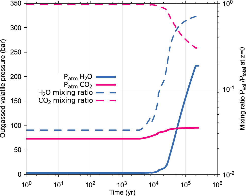
Figure 14. OLRTOA sampled on the (Tsurf,  ) space obtained using the lbl model. The detailed calculation of the values is found in the companion paper.
Download figure:
Standard image High-resolution image
The grid spans surface temperatures from 650 to 4000 K and water vapor surface pressures from 4 to 300 bar. It is irregularly spaced and denser over the temperature range where the highest rate of enrichment and outgassing takes place. This range is obtained by performing simulations using synthetic melting curves with the interior model coupled to the gray atmosphere model (see Figure 5). For ![${T}_{s}\in \left[1400,1800\right]$](https://content.cld.iop.org/journals/0004-637X/875/1/11/revision1/apjab08edieqn75.gif) K, the OLR was sampled with a resolution of 20 K, while a 100 K resolution was employed outside this range. The sampling is sparser (eight values) on the pressure axis for
K, the OLR was sampled with a resolution of 20 K, while a 100 K resolution was employed outside this range. The sampling is sparser (eight values) on the pressure axis for ![$P\in \left[\mathrm{4,300}\right]$](https://content.cld.iop.org/journals/0004-637X/875/1/11/revision1/apjab08edieqn76.gif) bar. In order to obtain the OLR values at intermediate (P, T) points of the above data set, a bilinear interpolation method was used (van Rossum & Drake 2001). In order to estimate the interpolation error, we compared the interpolated field with an independent set of intermediate data points obtained from the atmospheric model. The relative interpolation error amounts to between 1% and 10%. The maximum of 10% occurs at pressures lower than 10 bar and high temperatures. The minimum occurs for high pressures and temperatures at the lower end of the data set. Therefore, the quality of the result is acceptable for this study that focuses on the coolest end of the MO phase where the outgassed atmosphere has high pressure, and the errors are minimal (1–2 W m−2).
bar. In order to obtain the OLR values at intermediate (P, T) points of the above data set, a bilinear interpolation method was used (van Rossum & Drake 2001). In order to estimate the interpolation error, we compared the interpolated field with an independent set of intermediate data points obtained from the atmospheric model. The relative interpolation error amounts to between 1% and 10%. The maximum of 10% occurs at pressures lower than 10 bar and high temperatures. The minimum occurs for high pressures and temperatures at the lower end of the data set. Therefore, the quality of the result is acceptable for this study that focuses on the coolest end of the MO phase where the outgassed atmosphere has high pressure, and the errors are minimal (1–2 W m−2).
The data of Figure 14 represent the OLR at the TOA with a viewing angle of 38° and thus differ from the field shown in Figure 8, which represents the net planetary flux at the TOA. More details on the OLR value calculation can be found in the companion paper.
In order to satisfy the requirement of our iteration algorithm for surface temperatures lower than  = 647 K, which are not covered by our grid, we use a fit to the OLR data of (Nakajima et al. 1992). This aspect does not affect our results for the solidification process, which occurs for Tsurf ≈ TRF,0 ≫
  , but ensures that the iteration algorithm runs unhindered until convergence to the solution.
C.2. Limiting Radiation Values
We use Equation (18) to estimate the orbital distance for which a planet of a given albedo is located at the boundary that separates a long-term and short-term MO. To this end, the value of the limiting radiation Flim corresponding to a specific water vapor pressure  and rheology front temperature at the surface TRF,0 is needed. In Table 3, we report
  for two different rheology front surface temperatures as obtained by interpolating the OLR data points of the companion paper (Figure 14). The same values are plotted in Figure 10 and used to calculate the critical distances for the young Sun in Figure 11.
Appendix D: Constants
Table 4 includes the constants and parameters used in most of the simulations unless otherwise stated.
Table 4. Model Constants and Parameters
| Parameter | Value | Unit | Description |
|---|---|---|---|
| Rp | 6371 | km | Planetary radius |
| Rb | 3481 | km | Core–mantle boundary radius |
| g | 9.81 | ms−2 | Gravity acceleration |

|
0.01 | m2 kg−1 | Absorption coeff. at P0, T0 |

|
0.001 | m2 kg−1 | Absorption coeff. at P0, T0 |
| P0 | 101325 | Pa | Normal atmospheric pressure for k0,vol |
| T0 | 300 | K | Normal atmospheric temperature for k0,vol |
| α0 | 3 · 10−5 | K−1 | Mantle thermal expansivity |
| K0 | 200 | GPa | Mantle bulk modulus |
| K' | 4 | ⋯ | P-derivative of mantle bulk modulus |
| m | 0 | ⋯ | Parameter in Equation (3) |
| cP | 1000 | J kg−1 K−1 | Mantle isobaric thermal capacity |
| κT | 10−6 | m2 s−1 | Mantle thermal diffusivity |
| kT | κT/(ρcP) | J K−1 s−2 m−2 | Mantle thermal conductivity |
| ρl | 4000 | kg m−3 | Melt density |
| ρs | 4500 | kg m−3 | Solid density |
| ϕC | 0.4 | ⋯ | Critical melt fraction |
| η0 | 4.2 · 1010 | Pa s | Solid viscosity prefactor |
| E | 240 | kJ mol−1 | Activation energy |
| V | 5 | cm3 mol−1 | Activation volume |
| R | 8.314 | J mol−1 K−1 | Ideal gas constant |
| AG | 3.9759 | ⋯ | Prefactor in Equation (9) calibrated for basanite |
| BG | a | K | Parameter in Equation (9) |
| CG | a | K | Parameter in Equation (9) |
| AK | 0.00024 | ⋯ | Prefactor for hydrous liquid in Equation (8) |
| BK | 4600 | ⋯ | Parameter for hydrous liquid in Equation (8) |
| CK | 1000 | K | Parameter for hydrous liquid in Equation (8) |
| κH2O, pv | 1.0 · 10−4 | ⋯ | H2O partition coeff. in solid perovskite |

|
1.1 · 10−2 | ⋯ | H2O partition coeff. in solid lherzolite |
| κCO2, pv | 5.0 · 10−4 | ⋯ | CO2 partition coeff. in solid perovskite |

|
2.1 · 10−3 | ⋯ | CO2 partition coeff. in solid lherzolite |
Note.
aThe value of this parameter is dynamically calculated during the simulation.Download table as: ASCIITypeset image
Appendix E: Exoplanets
Table 5 includes the planet and host star parameters used in the calculations presented in Figure 12.
Table 5. Planet and Host-star Parameters Used in Figure 12
| Planet | Orbital Distance R | Host Star | Teff | Rstar | Luminosity L | References |
|---|---|---|---|---|---|---|
| (au) | (K) | (in solar units R⊙) | (in solar units L⊙) | |||
| aKepler 236 c | 0.1320 | Kepler 236 | 3750 | 0.510 | ⋯ | exoplanet.eu/catalog/ |
| 55 Cancri e | 0.0156 | 55 Cancri | ⋯ | ⋯ | 0.59 | exoplanet.eu/catalog/ |
| Earth | 1.0000 | Sun (100 Myr old) | 5326 | 1.000 | 0.72 | Gough (1981) |
| aKepler 36 b | 0.1151 | Kepler 36 | 5911 | 1.619 | ⋯ | openexoplanetcatalogue.com |
| aHD 219134 b & c | 0.0388 and 0.0653 | HD 219134 | 3131 | 0.186 | ⋯ | exoplanet.eu/catalog/ |
| aRoss 128 b | 0.0496 | Ross 128 | 3192 | 0.197 | ⋯ | openexoplanetcatalogue.com |
| aGJ 1132 b | 0.0154 | GJ 1132 | 3270 | 0.207 | ⋯ | openexoplanetcatalogue.com |
| aLHS 1140 b & c | 0.087 & 0.02675 | LHS 1140 | 4699 | 0.778 | ⋯ | openexoplanetcatalogue.com |
| aKepler 78 b | 0.01 | Kepler 78 | 5089 | 0.74 | ⋯ | exoplanet.eu/catalog/ |
Note.
aIn the absence of values of luminosity relative to L⊙, we calculated the stellar luminosity directly from Teff, RStar data.Download table as: ASCIITypeset image
Appendix F: Calibration of the Melt Viscosity Prefactor
The composition of anhydrous peridotite, which we employed to define our "synthetic" melting curves (a list of the corresponding oxides can be found in Hirschmann 2000), is not covered by the empirical model of Giordano et al. (2008) that we used to determine the liquid viscosity and its dependence on the water concentration (Section 2.6). However, we found that the composition of basanite that belonged to the Giordano & Dingwell (2003) and Giordano et al. (2008) model calibration database is able to reproduce the temperature-dependent viscosity values of anhydrous silicate obtained experimentally (Urbain et al. 1982) to within less than 10% relative error. To be consistent with the assumption of a peridotitic composition, it is important to use a composition as close to a primitive one as possible. Indeed, the composition of basanite is among the least evolved in the classification of melts (Le Bas et al. 1986).
Assuming such composition and fitting the model of Giordano et al. (2008) to the experimental data of Urbain et al. (1982) (see Figure 2), we obtained a modified prefactor in Equation (9), namely AG = −3.976. The result is within the acceptable range of AG = −4.55 ± 1 log unit, given by the model authors (Giordano et al. 2008). As shown in Table 6, the use of this prefactor yields an error relative to the experimental values smaller than 10%. Note that we use this calculation only to provide a first-order estimate of the effects of water on the melt viscosity without needing to explicitly describe the evolution of the melt composition, which is beyond the scope of the present work.
Table 6. Comparison between Values of the Viscosity of Anhydrous Liquid Peridotite Obtained Experimentally and Calculated with the Model of Giordano et al. (2008) Assuming a Basanite Composition and a Prefactor AG = −3.976 in Equation (9)
| T (K) | Experimental ηl (Pa s) | Calculated ηl (Pa s) | Error (%) |
|---|---|---|---|
| 2000 | 0.22 | 0.2350 | 6.84 |
| 2220 | 0.08 | 0.0788 | −1.47 |
| 2300 | 0.06 | 0.0579 | −5.01 |
Download table as: ASCIITypeset image
Appendix G: Radioactive Decay
Heat production due to long-lived radioactive elements 238U, 235U, 40K, and 232Th, and short-lived elements 26Al and 60Fe is taken into account in the energy balance Equation (4) via the term qr, the explicit expression of which reads

where, for each element i,  is the isotope concentration in the silicate mantle at the formation time of the CAI (4.55 Gyr ago), Qi the specific heat production, λi the half-life, t0 the assumed formation time of the MO (e.g., 2 or 100 Myr after the CAI as in experiment 4 in Table 2), and t the time (with t > t0). For the long-lived elements, the initial isotope concentration
  is calculated by scaling back in time its present-day concentration according to the isotope half-life. In Appendix G, Table 7, we report for each isotope the parameters of Equation (31). The energy released by the decay of the radioactive isotopes is made available to the whole MO volume.
Table 7. Parameters Used in Equation (31) to Compute the Radiogenic Heat Production
| Radioactive Isotope | Concentration X0 | Heat Production Q (W/kg) | Half-life λ (yr) |
|---|---|---|---|
| 238Ua | 6.23 · 10−8 | 9.46 · 10−5 | 4.47 · 109 |
| 235Ua | 1.97 · 10−8 | 5.69 · 10−4 | 0.704 · 109 |
| 40Ka | 4.61 · 10−7 | 2.94 · 10−5 | 1.25 · 109 |
| 232Tha | 1.54 · 10−7 | 2.54 · 10−5 | 14.5 · 109 |
| 26Alb | 1.23 · 10−6 | 0.455 | 0.717 · 106 |
| 60Feb | 7.2 · 10−10 | 0.0412 | 2.62 · 106 |
Notes.
aParameter values are from Schubert et al. (2001). bConcentrations from McDonough & Sun (1995). Heat productions and half-lives from Neumann et al. (2014).Download table as: ASCIITypeset image