


Abstract
We develop a new method to measure the 3D kinematics of the subphotospheric motion of magnetic elements, which is used to study the coupling between the convection-driven vortex motion and the generation of ubiquitous coronal waves. We use the method of decomposing a line-of-sight magnetogram from MDI/SDO into unipolar magnetic charges, which yields the (projected) 2D motion [x(t), y(t)] and the (half) width evolution w(t) of an emerging magnetic element from an initial depth of d ≲ 1500 km below the photosphere. A simple model of rotational vortex motion with magnetic flux conservation during the emergence process of a magnetic element predicts the width evolution, i.e., w(t)/w0 = [B(t)/B0]−1/2, and an upper limit of the depth variation d(t) ≤ 1.3 w(t). While previous 2D tracing of magnetic elements provided information on advection and superdiffusion, our 3D tracing during the emergence process of a magnetic element is consistent with a ballistic trajectory in the upward direction. From the estimated Poynting flux and lifetimes of convective cells, we conclude that the Coronal Multi-channel Polarimeter–detected low-amplitude transverse magnetohydrodynamic waves are generated by the convection-driven vortex motion. Our observational measurements of magnetic elements appear to contradict the theoretical random-walk braiding scenario of Parker.
Export citation and abstract BibTeX RIS
1. Introduction
Ubiquitous magnetohydrodynamic (MHD) waves have been discovered in the solar corona with the Coronal Multi-channel Polarimeter (CoMP) instrument (Tomczyk et al. 2007; Tomczyk & McIntosh 2009; Morton et al. 2015). These MHD waves have been detected from their line-of-sight velocity in the solar corona above the limb using the Fe xiii (10747 Å) line with the CoMP instrument. These waves exhibit upward propagation into a coronal height range of r ≈ (1.05–1.35)R⊙, phase speeds of vph ≈ 1000–4000 km s−1, and oscillating loops that appear to be coaligned with the magnetic field. The quasiperiodic transverse wave motion has a (mean root square) speed of v ≈ 0.3 km s−1 and typical periods of T ≈ 5 minutes, which produces relatively small transverse displacements of x = v T ≈ 100 km.
In comparison, kink-mode oscillations (standing waves), which generally are triggered by flares, coronal mass ejections, and/or eruptive filaments, display much larger (40 times) transverse amplitudes of x = 4100 ± 1300 km and transverse speeds of v ≈ 12 km s−1 (Aschwanden et al. 1999) and thus are easier to detect.
Because of this huge discrepancy in wave amplitude between these two cases, some physical conditions must be different in the excitation of transverse large-amplitude kink-mode waves as detected with the TRACE instrument and the low-amplitude Alfvénic kink-mode waves detected with CoMP, which has a high sensitivity to detect the Doppler shift of transverse loop oscillations. While the large-amplitude waves are obviously excited by Lorentz forces that occur in flaring and eruptive conditions, we argue in this paper that the low-amplitude waves as seen by CoMP are excited by convection-driven vortex motion at the photospheric footpoints of coronal loops. Since photospheric convection is self-organizing on granular scales (L ≈ 1000 km) and operates throughout the solar surface, an immediate prediction of this model is that Alfvénic waves, if they exist in the solar corona, should be ubiquitously distributed throughout the corona, because the driver, i.e., the convective motion, is ubiquitous in the quiet Sun's photosphere.
Tracking of magnetic features in the turbulent environment of magneto-convection in the photosphere has been carried out only recently, since automated feature recognition codes became available (Crockett et al. 2009; Keys et al. 2011). Abramenko et al. (2011) used an automated tracking code that traced the motion of bright points in the quiet Sun, a coronal hole, and an active region plage using a 1 nm bandpass TiO interference filter centered at a wavelength of 7057 Å with the Goode New Solar Telescope of Big Bear Observatory. The bright point proper motion was found to be consistent with superdiffusion on timescales of 10–300 s, spatial scales of ≳22 km, and diffusion coefficients of ≈12–12 km2 s−1 (Abramenko et al. 2011). Manso Sainz et al. (2011) tracked small magnetic structures in very quiet (internetwork) regions using the Fe i 6300 Å doublet lines of the Solar Optical Telescope (SOT) on board Hinode, with a cadence of 28 s over 2–6 hr and a spatial resolution of 0 3. They found initial advective motion of the tracked features with a characteristic mean velocity of ≈2 km s−1, while the features subsequently reach the intergranular lanes and remain there, being buffeted by the random flows of neighboring granules and turbulent intergranules, with a diffusion constant of 195 km2 s−1 on spatial scales of ≈250–1000 km (Manso Sainz et al. 2011, Figure 1 therein). Further studies tracked the diffusion of magnetic elements up to supergranular features with similar results, using the Na i D 5896 Å line of SOT/Hinode/NFI (Giannattasio et al. 2013; Stangalini et al. 2014; Iida 2016; Agrawal et al. 2018). Analysis of magnetic element motions in both Hinode observations and MURaM simulations (Agrawal et al. 2018) demonstrates that the observed superdiffusive scaling at very short temporal increments is caused by center-of-mass jitter induced by magnetic flux element evolution superimposed on the advective contribution of granulation. Moreover, for long temporal increments beyond the correlation time of granular flows, the motions reflect both the random granular contribution and the large-scale longer-lived supergranular advection. Thus, magnetic element motions cannot be interpreted as strictly advective or diffusive on either short or long timescales. Superdiffusive scaling results from mixed contributions to the element motions. Numerical simulations using SOT/Hinode data as boundary conditions detect coherent (rather than incoherent random) structures in photospheric turbulent flows (Chian et al. 2014). Using Interferometric Bidimensional Spectropolarimeter and SOT/Hinode data, it is found that the interpretation of the displacement spectrum is ambiguous and can be reproduced by either superdiffusion or advection (Caroli et al. 2015; Del Moro et al. 2015). Attie & Innes (2015) applied the novel method of "magnetic ball-tracking," which is able to detect and quantify flux emergence, as well as flux cancellation.
While all previous studies embark on 2D motion tracking, here we develop a new model that allows us to measure the kinematic motion of magnetic elements from magnetograms in 3D, probing the shallow depths of the solar subphotospheric convection zone. The kinematic motion of magnetic elements produces magnetic field fluctuations, which can be used to define the Poynting flux in the generation of Alfvénic waves that propagate into the corona, and this method can be used to predict the amplitude and periods of Alfvénic fast kink-mode waves in the solar corona and solar wind (VanKooten & Cranmer 2017). Evidence for buffeting-induced kink waves in solar magnetic elements has already been inferred from an empirical mode decomposition (EMD) analysis of the time series of magnetic element parameters (Stangalini et al. 2014). There is also observational evidence for (unnoticed) magnetic flux oscillations detected with IMaX/Sunrise, with periods close to granular lifetimes (Martinez Gonzalez et al. 2011). The new model mimics the subphotospheric convection on granular scales, which is linked to the field line braiding in Parker's nanoflare heating scenario.
The content of this paper includes a theoretical part on the 3D magnetic field modeling and estimates of the Poynting flux of convection-driven ubiquitous coronal MHD waves (Section 2), data analysis of measuring the 3D motion of magnetic elements using HMI/SDO magnetograms (Section 3), a discussion in the context of previous work (Section 4), and conclusions (Section 5).
2. Theoretical Model
2.1. Magnetic Potential Field
The simplest representation of a magnetic potential field that fulfills Maxwell's divergence-free condition (∇ · B = 0) and the current-free condition j = ∇ × B = 0 is a unipolar magnetic charge j (or centroid of a magnetic field distribution) that is buried below the solar surface, which entails a magnetic field Bj(x) that points (isotropically) away from the buried unipolar charge and whose field strength falls off with the square of the distance rj,
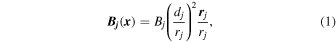
where Bj is the magnetic field strength at the solar surface above a buried magnetic charge, (xj, yj, zj) is the subphotospheric position of the buried charge, dj is the depth of the magnetic charge,

and rj = [x − xj, y − yj, z − zj] is the vector between an arbitrary location x = (x, y, z) in the solar corona (where we desire to calculate the magnetic field) and the location (xj, yj, zj) of the buried charge. We choose a Cartesian coordinate system (x, y, z) with the origin in the Sun center, and we are using units of solar radii, with the direction of z chosen along the line of sight from Sun center to Earth. For a location near disk center (x ≪ 1, y ≪ 1), the depth of the magnetic charge is dj ≈ (1 − zj). Thus, the distance rj from the magnetic charge is

The absolute value of the magnetic field Bj(rj) is simply a function of the radial distance rj (with Bj and dj being constants for a given magnetic charge),

From this expression, we can directly see the conservation of magnetic flux along a radially diverging flux tube with cross-section A(r) = r2, since the flux fulfills  .
.
The apparent full width at half maximum (FWHM) of the line-of-sight component Bz(x) profile can be calculated from the geometric diagram shown in Figure 1. We choose the x-axis at the photospheric level and bury a magnetic charge j at a depth dj, which has a line-of-sight component Bz(x = 0) = Bj at the photospheric level and is aligned with the vertical 3D magnetic field vector B = (0, 0, Bj). The radial field component Br(x = wj) intersects the photosphere at a distance x = wj, inclined by an angle θ from the vertical. The distance from the magnetic charge to the photosphere is rj, and the radial magnetic field at the photospheric level at the distance x = wj is Br(x = wj) = Bj (dj/rj)2, according to Equation (4). The corresponding line-of-sight component Bz(x = wj) is a factor of  smaller than the radial component Br(x = wj), i.e., Bz(x = wj) = Br(x = wj) cos θ, and thus has the value

which falls off with the third power of the distance rj. Thus, the half width wj is obtained by requiring Bj (dj/rj)3 = Bj/2, which yields, using the Pythagorean relationship  ,
,

This linear relationship means that the width wj is always proportional to the depth dj of the buried unipolar charge. Equation (6) is a very practical relationship because it allows us to directly predict the subphotospheric depth dj of a buried magnetic charge in a potential field model based on the apparent FWHM = 2wj ≈ 1.53 dj measured in a line-of-sight magnetogram.

Figure 1. Cross-section of a unipolar magnetic source M, showing the geometric relation between the half width wj and depth dj of a unipolar charge j. The line-of-sight direction is the (vertical) z-axis, and the (horizontal) direction is the x-axis. For the calculation of the line-of-sight profile Bz(x), see text.
Download figure:
Standard image High-resolution image2.2. Line-of-sight Magnetogram
We progress now from a single magnetic charge to an arbitrary number nm of magnetic charges and represent the general magnetic field with a superposition of nm buried magnetic charges, so that the potential field can be represented by the superposition of nm fields Bj from each magnetic charge j = 1, ..., nm,
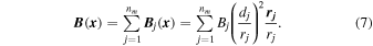
It is trivial to verify the condition of divergence-freeness for a magnetic field with multiple magnetic charges. Since the divergence operator is linear, the superposition of a number of divergence-free fields is divergence-free also,

and thus B is a potential field. Applications of this potential field model in the framework of magnetic charges can be found in a number of recent studies (e.g., Aschwanden & Sandman 2010; Aschwanden 2013, 2016; Warren et al. 2018).
Based on the superposition principle of magnetic charges (Equation (7)), a line-of-sight magnetogram Bz(x, y) can be created with an arbitrary number of (buried) unipolar magnetic charges, and vice versa; any line-of-sight magnetogram can be decomposed into a finite number of magnetic charges, i.e., [xj, yj, zj, Bj], j = 1, ..., nm. This inversion task can be accomplished by forward-fitting of the coordinates [xj, yj, zj] and field strengths Bj of the magnetic components (for an example, see Figure 3 in Aschwanden & Sandman 2010). Such a decomposition directly yields the subphotospheric depths dj for all magnetic components in a potential field model.
For the sake of simplicity, we formulate the following theoretical model for observations near disk center, but it can be generalized to arbitrary positions on the solar disk in a straightforward way (see the Appendix in Aschwanden et al. 2012).
2.3. Tracking the Subphotospheric Vortex Motion
The solar granulation has a typical scale of L ≈ 1000 km self-organized by the solar convection process (subject to the Rayleigh–Bénard instability) and is driven by a vertical temperature gradient (Lorenz 1963). As a consequence of the negative vertical temperature gradient, dT/dh < 0, circular vortex motions are expected in the vertical plane in the shallow depths of the solar convection zone. Besides the unmagnetized hydrodynamic fluids, we envision that magnetic elements are also generated in the solar convection zone and occasionally become entrained in a convective vortex whirl, where the magnetic element is first transported in the upward direction, then is advected in the horizontal direction toward intergranular lanes, and finally is buffeted in the network. The trajectory of a magnetic element may start near the midpoint at the bottom of a granule (Figure 2) and may end near the top of a granule, with subsequent advection into an intergranular lane.
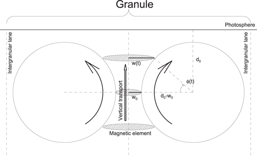
Figure 2. Diagram of a subphotospheric granule, which consists of two oppositely rotating convection cells (large circles) that squeeze the width w(t) of a magnetic element (hatched ellipses) to a minimum size of w0 during the vertical upward motion. The rotation angle is indicated with ϕ(t), the radius of a convection cell is r0 = d0 − w0, the depth of the center of the convection cells is d0, and the distance between the centers of the two convection cells is 2d0.
Download figure:
Standard image High-resolution imageA novel step of this study is that for the first time, we are going to use the subphotospheric depths measured from a time sequence of line-of-sight magnetograms Bz(x, y, t) by tracking the vortex motion of subphotospheric convection. We envision a simple geometric model of granular vortex motion where the strongest upflows occur in the midpoint of a granule. A cross-section of a granule is shown in Figure 2, which consists of two convective cell cross-sections that rotate in opposite directions so that emerging magnetic elements arise and emerge in the midpoint of a granule while they subsequently stream toward the edges of granules into intergranular lanes or toward the network.
The evolution of the magnetic field of a traced magnetic element generally exhibits a rise time when the magnetic field strength monotonically increases (t1 < t0 < t2) followed by a decay time when the magnetic field monotonically decreases (t0 < t < t2), which we interpret as compression and decompression phases of a magnetic element. The compression phase occurs when the magnetic element is sucked up between two counterrotating vortices (Figure 2), while the decompression phase occurs when the magnetic element arrives near the top of a granule. We found that the time evolution can be adequately characterized by a Gaussian function plus a constant background,
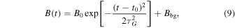
where τG represents a timescale that corresponds to the Gaussian (half) width.
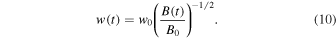
Applying the conservation of the magnetic flux during the vertical upward motion of the magnetic field during a compression phase, we can predict the time evolution of the width w(t) of a magnetic element, since the area varies as A(t) ∝ w(t)2, and conserving the magnetic flux Φ(t) = A(t) B(t) = const, the magnetic field varies B(t) ∝ A(t)−1 ∝ w(t)−2, or inversely as w(t) ∝ B(t)−1/2,
For the evolution of the depth d(t) of a magnetic element, we assume vertical transport from an initial depth d1 = d(t = t1) at a location below a granular convection cell, while the vertical transport ends at a final depth d2 = d(t = t2) above a granular convection cell near the photosphere (Figure 2). All depth locations d(t) during this vertical transport time interval are constrained by an upper limit duni(t) that is given by the width w(t) of the potential field of an unipolar point charge (Equation (6)),

Only in the deepest layers below the convection cells do we expect that the magnetic flux element is not affected by the compression of convection cells, where the depth can be estimated from the unipolar point charge depth, i.e., d1 ≈ 1.3 w1 at time t1, while the depth at the end of the emergence process is close to the photospheric height level. Interpolating the depth evolution between the bottom and top of a convection cell with a constant speed, we expect a linear depth variation d(t) with time,

where the (constant) vertical upward velocity vz is defined by

Thus, our simple analytical model (Equations (9)–(13)) of the vertical motion during the emergence of a magnetic element is constrained by the observed evolution of the magnetic field B(t), the (half) widths w(t), and the (largest) depth d1 = d(t = t1) = 1.3 w1 at the initial phase of the emergence process. The theoretical model makes two predictions: (i) the conservation of the magnetic flux (Equation (10)), and (ii) an upper limit of depths d(t) ≤ duni(t) ≈ 1.3 w(t) (Equation (11)). We will test these theoretical predictions in the following (Section 3.4). If the data match these theoretical relationships, the method of 3D tracking from line-of-sight magnetograms is strongly supported. The only assumptions that go into this model are the conservation of the magnetic flux and a constant velocity for the vertical upward motion of a magnetic element. We neglected horizontal motions (vx, vy) in our simple model here, but it can easily be included by tilting the vertical axis.
2.4. Poynting Flux of Convective Vortex Motion
In our model, we assume that magnetic elements are entrained into the convective vortex motion, which causes a magnetic field variation Bj(t) at the solar surface according to the square dependence of the subphotospheric depth dj(t) variation of the magnetic charge (Equation (4)). The associated variation in the magnetic pressure pm(t),

which corresponds to a variation in the magnetic energy Em(t),

where V is the spatial volume. We can define this volume from a 3D flux tube with a cross-sectional area A and a height corresponding to the density scale height λ of the solar corona,

In hydrostatic equilibrium, the density scale height λ of the solar corona is proportional to its temperature T,

We can now quantify the Poynting flux FP, which is an energy input per area A and time unit τ,

where τ is the lifetime of a granular vortex motion. The area dependence A cancels out and the scale height λ can be replaced by the mean coronal temperature Te,
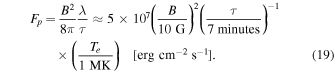
This estimated Poynting flux, which is produced ubiquitously over the photospheric solar surface, is several orders of magnitude above the heating requirement for the quiet Sun or coronal holes, which is Fp = 3 × 10⁵ erg cm−2 s−1 for the quiet Sun and Fp = 8 × 10⁵ erg cm−2 s−1 for a coronal hole, respectively (Withbroe & Noyes 1977). Thus, we conclude that dissipation of the convection-driven generation of Alvénic waves by only ≈1% is sufficient to heat the quiet Sun or coronal holes, while the remainder of the injected Poynting flux is available to heat the chromosphere and accelerate the solar wind.
2.5. Alfvénic Loop Oscillations
In our model, the footpoint motion of coronal loops is dictated by the vortex motion of the solar granulation, which for typical values (L ≈ 1000 km, τ ≈ 7 minutes) produces a velocity of v ≈ (L/2)/τ ≈ 1 km s−1, similar to the observational result of vobs ≈ 0.3 km s−1 inferred from CoMP data (Tomczyk et al. 2007).
Transverse kink-mode oscillations are expected when the phase speed matches the resonance condition of the Alfvénic loop crossing times. The Alfvén speed is
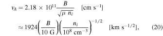
where μ = 1.27 is the mean molecular weight and ni is the ion density. The kink speed is
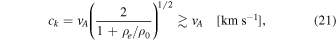
where ρ0/ρi is the inner to the outer density ratio. The kink-mode period is given by the kink-speed crossing time,

From this resonance condition of the kink-speed crossing time, we can express the magnetic field strength B as a function of the loop length L, the kink-mode period Pkink, and ion density ni,
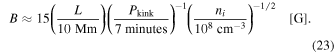
In our model, we consider the convective vortex motion with a mean period of Pmin ≈ 7 minutes as an exciter of kink-mode oscillations. From the relation (Equation (20)), we predict that the typical magnetic field is B ≈ 15 G (for a loop length of L ≈ 10 Mm).
3. Data Analysis and Results
3.1. Data Selection
For the data analysis of our project on determining the 3D trajectories of magnetic elements in the quiet Sun, we select an HMI/SDO magnetogram (file type hmi_M_45 s) at an arbitrary time (2010 June 19, 01:27:42 UT). We extract a time sequence of 26 HMI images after the starting time of 01:27:42 UT with an HMI cadence of 45 s, which covers a time interval of 1170 s (19.5 minutes), ending at 01:47:12 UT.
From the full-disk images, we select a small field of view (0.1 R⊙) near disk center (making sure that it does not contain any active region). The chosen field of view is at heliographic longitude and latitude N00E00, which corresponds to the Cartesian coordinates x1 = −17.4, x2 = +17.4, y1 = −35.0, and y2 = −0.48 Mm with respect to Sun center. The HMI images have a pixel size of 05 (or 362 km). Because HMI magnetograms with full resolution turned out to be too noisy for the purpose of our project, we rebin them by a factor of two into macropixels with a size of 2 × 2 pixels (with 10 or 725 km resolution). The field of view of 0.1 R⊙ then contains a subimage with a size of 47 × 47 macropixels. Coaligment between the HMI images is assumed to be of subarcsecond accuracy. We eliminate the solar rotation by correcting for the synodic rotation period of Tsyn = 27.2753 days, which amounts to an incremental shift of Δx ≈ 84 km for an HMI cadence of 45 s.
3.2. Decomposition of Magnetograms
The next analysis step is the decomposition of magnetograms into a finite number nm of unipolar magnetic charges, which are each characterized by four parameters: the spatial 3D coordinates [xj, yj, zj]; j = 1, ...; nm; and the magnetic field strength Bj at the photospheric surface vertically above the location of each magnetic charge. These physical parameters [Bj, xj, yj, zj], are obtained from the inversion of the observables [Bz, xp, yp, wp], where [xp, yp] is the projected 2D position of a local peak value of the line-of-sight magnetic field component Bz, and wp is the apparent FWHM of a magnetic element. The technical details of this inversion are given in the Appendix of Aschwanden et al. (2012) and Aschwanden (2016). From the decomposition of the time sequence of nt = 26 magnetograms into nm = 200 magnetic components and np = 4 parameters each, we obtain a total of nt × nm × np = 20,800 (automatically) measured parameters [B(t, m), x(t, m), y(t, m), z(t, m)], t = 1, ..., nt, m = 1, ..., nm. The number of magnetic components nm corresponds to a threshold of the minimum magnetic field strength in the model and is typically chosen at three standard deviations above the noise level.
3.3. 3D Tracking of Magnetic Elements
From the nt × nc = 5200 magnetic elements that we extracted from the magnetograms during nt = 26 time steps and nc = 200 local peaks in each Bz(x, y) magnetogram, we group the cospatial locations sampled at various times into a set of unique locations (xi, yi), i = 1, ..., ni that have a minimum separation (of two full widths) from each other and a field strength above a threshold Bthresh that corresponds to three standard deviations of the background magnetic field fluctuations. The minimum separation distance of two full widths is an empirical criterion that optimizes the separation versus the clustering of substructures in magnetic elements. While the analytical model is shown in Figure 3, the observed line-of-sight magentograms of three cases are shown in Figures 4(g), 5(g), and 6(g), where a crosshair marks the unique location of each of the three magnetic elements, and a circle indicates the area with a radius that corresponds to the minimum separation between different unique source locations. Figures 4–6 show the (smoothed) propagation distance in the x-direction x(t) (Figures 4(a), 5(a), and 6(a)) and y-direction y(t) (Figures 4(b), 5(b), and 6(b)), upper limits on the depths of the magnetic elements d(t) (Figures 4(c), 5(c), and 6(c)), widths of the magnetic elements w(t) (Figures 4(d), 5(d), and 6(d)), magnetic field strength B(t) (Figures 4(e), 5(e), and 6(e)), and projected source motion y(x) (Figures 4(f), 5(f), and 6(f)).The spatial propagation distance shown in Figures 4–6 is smoothed with a boxcar of five time steps, which is 5 × 45 s = 225 s for the HMI cadence. A 1D scan of the magnetogram that goes through the center of the magnetic element is also shown (Figures 4(h), 5(h), and 6(h)), along with a Gaussian fit that provides the width measurements w(t).
Let us describe the measurements of the first example in more detail (Figure 4). The automated detection algorithm finds a magnetic element from the location (xp, yp) of the absolute maximum (peak) field strength (Figure 4(g)). The magnetic field variation B(tp, xp, yp) at this location is tracked (within a radius of two FWHM) in time, B(t) (Figure 4(e)), starting from the peak time tp to the start time ts (at the first minimum value to the left), as well as to the end time te (at the first minimum value to the right). This encompasses the time range from ts = 400 to te = 1120 s in this example (Figure 4(e)). The structure seen before at time t < 400 s is considered to be a separate structure. The algorithm then eliminates the first detected structure from subsequent searches of smaller magnetic elements.
The measured FWHM of the automatically detected magnetic elements (see Figures 4(h), 5(h), and 6(h)) are listed in Table 1 (second column), having a mean and standard deviation of FWHM = 1373 ± 440 km, or 19 ± 06, which is twice the value of the 2 × 2 macropixels we used from the HMI magnetograms. Thus, it appears that these magnetic features are spatially resolved. If the features were unresolved, we would expect that (i) the measured width is equal to the HMI macropixel resolution of 725 km, (ii) the width w(t) as a function of time should be a constant with this value of 725 km, and (iii) the predicted and observed width profile w(t) should be uncorrelated, i.e., have a low cross-correlation coefficient of CCC ≲ 0.5, which is not the case (see Figures 4(d), 5(d), and 6(d) and Table 1). Of course, this does not mean that the magnetic counterparts of the granules envisioned in our model (Figure 2) are spatially resolved in the HMI magnetogram, but since we derive all our measurements from the HMI magnetogram, rather than from optical images where granules are visible, the spatial scale of granules does not explicitly enter our analysis.
Table 1. Statistical Measurements of 14 Magnetic Elements: L2 = 2D Propagation Distance, τ = t2 − t1 Time Duration, v2 = the Mean 2D Horizontal Velocity, vz = the Vertical Velocity vz, Bsig = Standard Deviation of Magnetic Field Strength Fluctuations, Bmax = Maximum Magnetic Field Strength, CCCw = Cross-correlation Coefficient of Observed and Predicted Widths
| No. | FWHM | L2 | τ | v2 | vz | Bsig | Bmax | CCCw |
|---|---|---|---|---|---|---|---|---|
| (km) | (km) | (s) | (km s−1) | (km s−1) | (G) | (G) | ||
| 1 | 1237 | 476 | 720 | 0.7 | 1.8 | 12.7 | 235.1 | 0.82 |
| 2 | 1152 | 735 | 540 | 1.4 | 2.0 | 12.8 | 178.2 | 0.77 |
| 3 | 1252 | 740 | 315 | 2.4 | 2.5 | 12.3 | 150.1 | 0.88 |
| 4 | 1093 | 690 | 360 | 1.9 | 3.1 | 12.7 | 116.9 | 0.51 |
| 5 | 1358 | 437 | 405 | 1.1 | 1.8 | 11.7 | 78.2 | 0.55 |
| 6 | 1108 | 618 | 270 | 2.3 | 3.1 | 11.4 | 62.5 | 0.88 |
| 7 | 1696 | 751 | 585 | 1.3 | 1.8 | 12.8 | 55.1 | 0.81 |
| 8 | 1104 | 708 | 360 | 2.0 | 2.6 | 12.1 | 53.2 | 0.67 |
| 9 | 1301 | 349 | 270 | 1.3 | 2.8 | 11.9 | 51.7 | 0.86 |
| 10 | 1331 | 338 | 180 | 1.9 | 1.4 | 11.9 | 50.7 | 0.55 |
| 11 | 1132 | 474 | 225 | 2.1 | 4.0 | 12.7 | 42.7 | 1.00 |
| 12 | 1525 | 1273 | 450 | 2.8 | 1.3 | 12.0 | 39.2 | 1.00 |
| 13 | 2782 | 1416 | 405 | 3.5 | 1.9 | 12.5 | 38.8 | 1.00 |
| 14 | 1164 | 117 | 270 | 0.4 | 2.5 | 11.7 | 36.0 | 1.00 |
| 1373 | 652 | 382 | 1.8 | 2.3 | 12.2 | 84.9 | 0.81 | |
| ±440 | ±349 | ±150 | ±0.8 | ±0.8 | ±0.5 | ±61.8 | ±0.18 |
Note. The averages and standard deviations are indicated at the bottom of the table.
Download table as: ASCIITypeset image
3.4. Tests of Theoretical Predictions
We are now testing two theoretical predictions of our simple model of the emergence of a magnetic element (Figure 3). From the measured magnetic field evolution B(t) with a peak value of B0 = B(t = t0) at the peak time t0, magnetic flux conservation predicts an evolution of the (half) width of a magnetic element according to Equation (10),
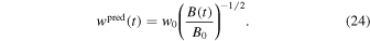
The Gaussian function of the magnetic field variation B(t) (Equation (9)) is shown in Figures 4(e), 5(e), and 6(e) (indicated by the data points with diamonds and the fitted Gaussians with red curves). The predicted widths wpred(t) are shown in Figures 4(d), 5(d), and 6(d)), also with red curves. In order to quantify the consistency between the two time profiles, we calculate the cross-correlation coefficient CCCw,
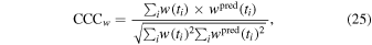
for which we find values of CCCw = 0.82, 0.77, and 0.88 (Figures 4(d), 5(d), and 6(d)) for the three magnetic elements 1, 2, and 3. Therefore, the observed w(t) and theoretically predicted widths wpred are highly correlated and confirm the magnetic flux conservation during the emergence of a magnetic element.
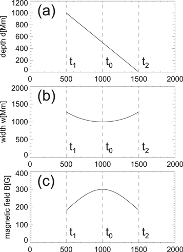
Figure 3. Analytical model of the vertical transport of a magnetic element, which includes the depth d(t) (a), the half width w(t) (b), and the variation of the magnetic field B(t) (c), based on magnetic flux conservation and constant velocity. The model parameters are B0 = 300 G, w0 = 1000 km, d0 = 1500 km, t1 = 500 s, t0 = 1000 s, and t2 = 1500 s.
Download figure:
Standard image High-resolution image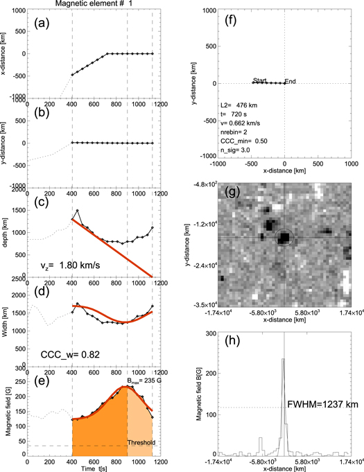
Figure 4. (a) Time variation of the x-coordinate x(t) and (b) y-coordinate y(t), (c) an upper limit of the depth d(t) (diamonds), (d) the observed width w(t), (e) the magnetic field B(t) at the photospheric level with a threshold of 3σ (dashed line), (f) the 2D motion y(x), (g) the HMI/SDO magnetogram, and (h) a scan Bz(x). The red curves represent the theoretical predictions of a constant velocity (c) and magnetic flux conservation model (d). The crosshairs indicate the location of the traced magnetic element, and the circle marks the separation radius between two adjacent magnetic elements (g).
Download figure:
Standard image High-resolution imageOur second theoretical prediction is that the width evolution w(t) of a magnetic element during emergence (Figure 3) provides an upper limit on the depth of the magnetic element, i.e., d(t) ≤ 1.3 w(t), according to Equation (6). Assuming that the width of a magnetic element is not squeezed by convective vortex motion at depths below the convection cells, in particular at the start time t1 of vertical transport, we have a depth measurement of d1 = d(t = t1) = 1.3 w(t1) = 1.3 w1. At the end of the vertical transport, when the magnetic element arrives at photospheric levels, the final depth is very shallow, i.e., d2 ≈ 0. Connecting these two depth values d1 and d2 with a constant velocity, we obtain a linearly decreasing depth evolution d(t), which is marked with a red curve in Figures 4(c), 5(c), and 6(c). The test of our theoretical model is whether the predicted depth evolution, i.e., dpred(t) = vz (t2 − t) (Equation (12)), fulfills the inequality of the observed upper limits d(t) ≤ dpred(t) at all times during the interval [t1, t2], which is indeed found to be the case (Figures 4(c), 5(c), and 6(c)), while equality is found to extend over a depth range of d ≈ 500–1500 km. The initial depths are found to be d ≈ 1500 (Figure 4(c)), 1000 (Figure 5(c)), and 800 km (Figure 6(c)).
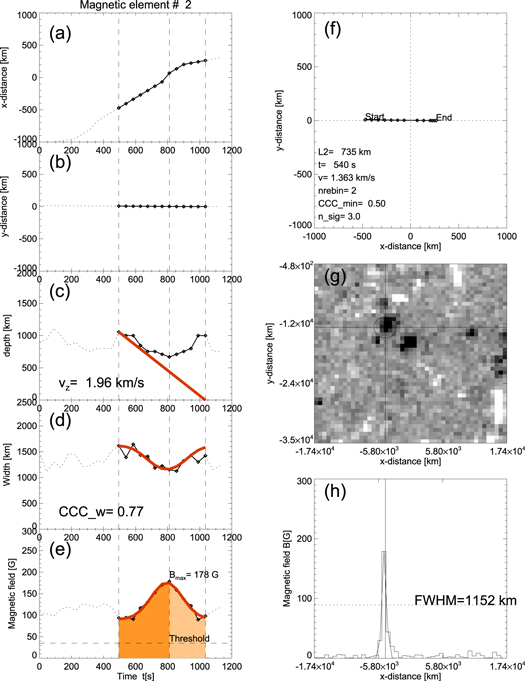
Figure 5. Representation similar to Figure 4 but for the second-strongest magnetic element, no. 2.
Download figure:
Standard image High-resolution image
Figure 6. Representation similar to Figures 4 and 5 but for the third-strongest magnetic element, no. 3.
Download figure:
Standard image High-resolution image
3.5. Statistics of Magnetic Elements
We perform statistics of magnetic element tracking in an area the size of 0.1 R⊙ during a total time duration of ≈20 minutes and find a total of ni = 14 magnetic elements that have a maximum magnetic field strength above a threshold level of three standard deviations of the unsigned magnetic field strength; in addition, we match a depth cross-correlation coefficient of CCCw ≥ 0.5. The statistical parameters of these 14 magnetic elements are listed in Table 1, which provides typical values for comparisons.
The tracked 2D distance of a magnetic element is found to be L2 = 650 ± 350 km, which is close to the half value of a canonical granule size (Lgran/2 ≈ 500 km), as expected for emergence near the center of a granule.
The mean duration of a magnetic element trajectory is τ = 380 ± 150 s (or τ = 6.4 ± 2.5 minutes). This agrees well with the canonical lifetime of granules (≈7 minutes), which is expected for the duration of coherent transport in a convective vortex. Note that the duration of a coherent event is characterized by a coherent rise and decay time of the magnetic field evolution B(t). In our measurement technique, the evolution of the magnetic field B(t) starts with a minimum B1 = B(t = tstart), peaks at Bmax = B(t = tpeak), and ends with a subsequent minimum B2 = B(t = tend), which defines the observed duration τ = tend − tstart.
The average velocity is found to be v2 = 1.8 ± 0.8 km s−1 for the horizontal motion and vz = 2.3 ± 0.8 km s−1 for the vertical motion. These values are close to previously obtained values, i.e., v ≈ 2 km s−1 (Manso Sainz et al. 2011).
The noise in the magnetogram corresponds to a standard deviation of the unsigned field strength of Bsig = 12.2 ± 0.5 G, from which we set a threshold of Bthresh = 3 Bsig = 36.3 G. Similar values for the standard deviation of the unsigned magnetic field strength were obtained by others, e.g., Bsig = 11.8 G (DeForest et al. 2007). Above this level, we found 14 magnetic elements with peak field strengths of 36 G ≲ Bmax ≲ 235 G. Setting a lower limit of CCCw > 0.5, we found mean cross-correlation coefficients of CCCw = 0.81 ± 0.18.
3.6. Poynting Flux of Convective Motion
We are now in a position to estimate the Poynting flux of the subphotospheric convection based on our measurements. From the magnetic field profiles B(t) of the various magnetic elements, we have to separate the motion-related magnetic field component Bmotion(t) and the stationary equilibrium magnetic field component Bstat(t),

The motion-related component Bmotion induces an apparent variability of the magnetic field due to the subsurface motion of magnetic elements driven by the rolling granular vortex motion, which is apparent as magnetic flux emergence, advection, or submergence. In contrast, the stationary component Bstat represents an equilibrium between the generation of magnetic flux and the energy loss of magnetic fields by transport from the photosphere to chromospheric and coronal structures, for instance, by Alfvénic waves. While we modeled the motion-related time-variable magnetic field Bmotion(t) by automated detection of emerging magnetic elements, we can estimate the stationary component from the background magnetic field, which we found to have a mean and standard deviation of Bbg = 12.2 ± 0.5 G (Table 1). The replenishment time of the stationary magnetic field can be estimated from the lifetime of a granule, which is equivalent to the duration of a magnetic element for which we measured a mean value of τ = 6.4 ± 2.5 minutes (Table 1). Inserting these values of Bbg = 12.2 G, τ = 6.4 minutes, and a coronal temperature of T = 1.0 MK into the expression of Equation (20), we obtain a Poynting flux of Fp ≈ 7 × 10⁷ erg cm−2 s−1 (at the base of the corona). Interestingly, only ≈1% of this energy is needed to heat the quiet-Sun corona or coronal holes, leaving ample energy to also heat the chromosphere and compensate for the solar wind, radiative, and conductive energy losses.
4. Discussion
We discuss the methods of 2D (Section 4.1) and 3D (Section 4.2) tracking of magnetic elements, advective versus diffusive transport (Section 4.3), the convection-driven Poynting flux and generation of ubiquitous Alfvénic waves (Section 4.4), and Parker's braiding scenario of coronal heating (Section 4.5).
4.1. 2D Tracking of Magnetic Elements
A new method of this study is the capability of tracking magnetic elements in 3D Euclidean space, i.e., measuring the trajectories [x(t), y(t), z(t)] of the center of magnetic elements below the solar photospheric surface, assuming a potential or slightly nonpotential magnetic field model. To our knowledge, all previous tracking methods were restricted to track magnetic features on the solar surface, which represents a 2D projection of the true 3D trajectory (e.g., Crockett et al. 2009; Keys et al. 2011). Abramenko et al. (2011) detected and tracked bright point features in the photosphere using a method described in Abramenko et al. (2010). The method takes advantage of the small size, enhanced intensity, and strong gradient in intensity around bright points and employs smoothing, unsharp-marking, and thresholding. Manso Sainz et al. (2011) manually detected and tracked small loop footpoints, following their dual appearance with opposite polarities at the two ends of a linear polarization region above some threshold. Since the loop footpoints are confined to the photosphere and chromosphere, this method essentially yields 2D trajectories. Giannattasio et al. (2013) implemented an iterative procedure that resolves both weak and strong peaks of magnetic features in magnetograms, while a segmented temporal sequence is then used to reconstruct the trajectories of magnetic features, which also yields 2D trajectories. Stangalini et al. (2014) used the "Yet another Feature Tracking Algorithm" (YAFTA) (Welsch & Longcope 2003; DeForest et al. 2007), which identifies and tracks magnetic pixels belonging to the same local maximum in magnetograms with the downhill method and yields 2D trajectories. Using the YAFTA code with corrections to properly account for interactions of magnetic elements, Gošic et al. (2014) showed that internetwork regions are the main source of flux for the network. In addition to this, Gošic et al. (2016) described in a consistent way for the first time how individual supergranular cells gain and lose magnetic flux. Iida (2016) used the clumping method of Parnell et al. (2009). Agrawal et al. (2018) used a semiautomated procedure to track and verify magnetic flux elements, a combination of the downhill and the clumping method of Parnell et al. (2009). In summary, since all previous codes track features from photospheric line-of-sight magnetograms, preferentially near disk center, the tracked paths are 2D trajectories [x(t), y(t)], while no information on the third-dimension z(t) has been retrieved.
4.2. 3D Tracking of Magnetic Elements
In contrast, the decomposition method of a line-of-sight magnetogram into unipolar magnetic charges (Sections 2.1 and 2.2) yields information on the third coordinate z(t) of a unipolar charge (or magnetic element). For the sake of simplicity, we use the simplest kinematic model of the source motion of a magnetic element, namely the vertical upward motion in the center of a granule. There are two effects that come into play in this scenario. The first basic effect is that a unipolar magnetic charge in a potential field represents a self-similar geometry that implies a universal ratio of  between the apparent (half) width w of a line-of-sight component Bz(x) and the depth d of the unipolar magnetic charge. In the absence of motion, the depth d of a unipolar charge can be directly predicted from the observed width w. Even in the presence of translational motion, the same prediction holds. The second effect, however, when the motion of a magnetic element occurs in a flux tube with varying cross-section (in space and time), leads to a change in the magnetic field strength according to the magnetic flux conservation law, in order to maintain the divergence-freeness of a potential field. We successfully tested the magnetic flux conservation law in a vertical flux tube that is located between two counterrotating vortices of a granulation cell by comparing the observed width variation w(t) with the theoretically predicted width variation wpred ∝ B(t)−1/2. The relationship duni(t) ≈ w(t)/0.766 provides only an upper limit on the depth d(t), while the true depth can be approximately estimated from the vertical upflow velocity vz that is consistent with the upper limit d(t) = vz (t2 − t) ≤ duni(t), which is constrained by the start time t1, end time t2, maximum velocity vz = d1/(t2 − t1), and initial depth d1.
A caveat of our method is that we cannot distinguish between compression of a magnetic element (as modeled with conservation of the magnetic flux in our kinematic model) and other interaction processes with the given HMI spatial resolution (e.g., magnetic field annihilation), but future work with higher-resolution (016) NFI/Hinode and SOT data is in progress.
Our method probes typical depths of d ≈ 500–1500 km for magnetic elements, while larger structures (such as sunspots) are anchored further down. There are also tomographic inversion methods of features in subphotospheric depths in helioseismology (Kosovichev 1999), based on the inversion of sound-speed deviations from the numerous (standing) harmonic p-modes, which is mathematically much more challenging than our simple method that merely requires width measurements of (separated) magnetic elements in photospheric magnetograms.
4.3. Advection or Superdiffusion?
What do we learn about the subphotospheric motion of magnetic elements? A major question in this regard is whether magnetic elements are just passively carried by advection or perform a random walk with diffusive, subdiffusive, or superdiffusive characteristics. Most studies conducted displacement measurements (Δl)2(τ) ∝ τγ and determined whether the diffusion coefficient is subdiffusive (γ < 1), diffusive (γ = 1), superdiffusive (γ > 1), or ballistic (γ = 2), which is identical to advection along a straight line. Several studies found a superdiffusive regime (γ = 1.48–1.67: Abramenko et al. 2011; γ = 1.20–1.34: Giannattasio et al. 2013, Caroli et al. 2015; γ = 1.48: Agrawal et al. 2018). Giannattasio et al. (2013) found superdiffusion by granular motions on temporal scales shorter than 35 minutes, while features with longer timescales are trapped in network regions. Others found two regimes with the initial passive advection and subsequent random walk buffeted by granules (Manso Sainz et al. 2011). Long-term observations were carried out over 5 days and revealed superdiffusion for small scales and subdiffusion on larger scales (Iida 2016).
Superdiffusion can also be expressed with a turbulent diffusion coefficient as a function of scale (Abramenko et al. 2011). The diffusing structures, however, are not structured randomly but rather exhibit coherent structures that self-organize in photospheric turbulent flows (Chian et al. 2014). A debate originated as to whether superdiffusivity is generated by a turbulent dispersion process or by the advection due to convective patterns (Del Moro et al. 2015). Simulations of passive tracers in a Voronoi network exhibit a superdiffusive displacement spectrum that can be generated by a competitive advection process (Del Moro et al. 2015). The horizontal motions of photospheric intergranular bright points have also been studied by MURaM and ROUGH simulation codes using bright points as passive tracers, which reproduce the observed power spectrum (Van Kooten & Cranmer 2017).
The motions measured here are not strictly motions, since the magnetic field evolution plays a role. The observed superdiffusive scaling is a consequence of multiple processes occurring, advection and field evolution at the smallest temporal increments, and granular diffusion and supergranular advection at long temporal increments.
In our model of the 3D motion of magnetic elements, we infer a vertical upward motion during the initial emergence phase. This motion pattern in a vertical plane is consistent with previous measurements of advection, which supposedly occurs from the center of a granule to its edge (or intergranular lane). Our analysis also provides the depth range of vortex motion, which is initially found at d ≲ 1500 km below the photosphere for the largest magnetic element analyzed here (Figure 4(c)). Thus, we can conclude that the magnetic elements traced here are consistent with advection or ballistic motion during the observed lifetime (of τ ≈ 7 minutes), while a possible diffusive phase after the advective motion to the next intergranular lane cannot be measured here due to the limited spatial resolution of HMI magnetograms and is left to other high-resolution instruments, such as Hinode/NFI, SOT, and DKIST.
4.4. Convection-driven Generation of Transverse MHD Waves
Since the solar granulation pattern is covering the entire Sun (except in sunspots), we can assume that the existence of convection-driven vortex motion is a ubiquitous energy source for the overlying photosphere, chromosphere, and corona. The generation and maintenance of granule sizes ≈1000 km, as well as their characteristic lifetime of ≈7 minutes, is the result of a self-organizing process according to the Lorenz (1963) model driven by the upward-directed, negative temperature gradient in the convection zone. Note that self-organizing processes (without criticality) do not produce scale-free power-law distributions (of their length scale, timescale, or energy), as they are produced by self-organized criticality systems, but rather show "peaked" distributions with a preferred spatial and temporal scale, such as the canonical granule size of ≈1000 km. For a review of self-organization processes in solar and astrophysics, see Aschwanden et al. (2018).
A consequence of the ubiquitous convective vortex motion is the coupling of subphotospheric convection to resonant structures in the solar corona, such as fast kink MHD waves and slow magnetoacoustic waves. It has been shown previously that the rapid footpoint motion due to turbulent granular buffeting can effectively excite kink waves that can propagate upward and couple with longitudinal waves (Kalkofen 1997; Hasan et al. 2003). Observational evidence for buffeting-induced kink waves in solar magnetic elements has been recently demonstrated by the EMD of the time series from the motion of magnetic elements (Stangalini et al. 2014). With this method, they found that the eigenmodes consist of subharmonic oscillations of a fundamental period of P = 7.6 ± 0.2 minutes. Since this period is close to the characteristic temporal scale of the photospheric convection cells, it was argued that these oscillations are associated with buffeting-induced oscillations (Stangalini et al. 2014). There is also evidence for magnetic flux oscillations from IMaX/Sunrise observations with periods close to granular lifetimes (Martinez Gonzalez et al. 2011), which appears to be consistent with the oscillations detected with the eigenmode decomposition analysis of Stangalini et al. (2014).
In our analysis, we measured for the magnetic elements a mean lifetime of τ = 6.4 ± 2.5, mean 2D spatial propagation distance of L2 = 650 ± 150 km, and mean velocity of vw = 1.8 ± 0.8 km s−1. If we couple these features of magnetic elements analyzed here with the footpoints of coronal loops, we expect that this coupling can excite transverse waves in coronal loops with similar periods τ and transverse displacements L2. Most of the coronal loops in the quiet Sun and active regions are located in closed-field configurations and thus are closed loops and can be resonant with upward-propagating MHD waves. We derived a typical loop length of L ≈ 10,000 km, timescales of P ≈ 7 minutes, and mean magnetic field strengths of B ≈ 15 G (Equation (23)). Ubiquitous MHD waves have been detected with CoMP, which revealed transverse velocities of x ≈ 100 km and periods of P ≈ 5 minutes (Tomczyk et al. 2007). Based on the agreement of these mean parameters (transverse wave speed, kink period, ubiquity), we propose that the small-amplitude waves detected with CoMP are coupled with the subphotospheric magnetic elements analyzed here from HMI/SDO magnetograms.
4.5. Parker's Braiding Scenario
Our kinematic analysis of subphotospheric magnetic elements also has far-reaching consequences for coronal heating models. For instance, the "magnetic field braiding" scenario of Parker (1983, 1988) suggests that the X-ray corona is created by the dissipation of the many tangential discontinuities arising spontaneously in the bipolar fields of the active regions of the Sun as a consequence of the random continuous motion of the footpoints of the field in the photospheric convection. This concept implies that the field lines become increasingly more twisted and braided by the random motion of the footpoints. Our kinematic analysis of magnetic elements, however, reveals that the magnetic elements undergo flux emergence within a timescale that is commensurate with the lifetime of a convection cell, which is only ≈7 minutes. Furthermore, we find that the horizontal and vertical motion caused by advection is nearly ballistic, rather than a diffusive random walk. These two arguments of the short lifetime and ballistic (nondiffusive) motion of magnetic elements contradict Parker's scenario of long lifetimes of line-tied magnetic field lines and their continuous random-walk braiding. In other words, (i) the footpoint motion of coronal loops is assumed to be a 2D random walk in Parker's model, while our measurements reveal ballistic transport of the 3D trajectory in a vertical plane; and (ii) the lifetime of a loop is assumed to be sufficiently long to enable significant braiding (across many granule diameters) in Parker's model, while our measurements reveal a ballistic vertical upward motion that does not last longer than a transit time across a granular diameter. In addition, the divergence- and force-freeness (of Maxwell's equations) that define a valid solution of the coronal magnetic field (during slow braiding) predict small misalignment angles between adjacent field lines, a property that is strongly violated in the cartoon published in Parker (1983; Figure 1) showing a strongly "kinked" flux tube surrounded by straight "unkinked" flux tubes. In summary, it appears that the assumptions of Parker's braiding scenario are not consistent with the observations and data analysis presented here.
5. Conclusions
In this study, we developed a method to measure for the first time the 3D kinematics of the subphotospheric motion of magnetic elements, which is used to demonstrate the convection-driven generation of ubiquitous coronal MHD waves. We summarize the main conclusions as follows.
- 1.The 3D coordinates (x, y, z) of subphotospheric magnetic elements can be traced from a magnetic potential field model that uses the decomposition of a line-of-sight magnetogram into a finite number of unipolar magnetic charges. Repeating this process as a function of time for a sequence of magnetograms yields the time-dependent kinematics [x(t), y(t), z(t]) of magnetic elements. Previous tracking of magnetic elements was exclusively carried out in 2D, [x(t), y(t)], while we use here for the first time a 3D method using the decomposition into unipolar magnetic charges in order to map out the third-dimension z(t). We find that unipolar magnetic elements can be probed in a depth range of d ≲ 1500 km.
- 2.Our emerging magnetic flux model makes two theoretical predictions: the magnetic flux conservation law that yields a correlation of the magnetic field strength with the width of a magnetic element, i.e., w(t) ∝ B(t)−1/2, and the upper limits of the depths of unipolar magnetic elements, d(t) ≤ w(t)/0.766, both of which we tested successfully from a sample of 14 magnetic elements using HMI data.
- 3.We estimate the Poynting flux of convective vortex motion, FP = B2λ/(8πτ), which depends on the mean background magnetic field strength, B ≈ 12 G; the lifetime of a magnetic element, τ ≈ 7 minutes; and the coronal temperature, Te ≈ 1.0 MK. Only about 1% of this Poynting flux is needed for the heating of the quiet Sun or coronal holes, while the remainder is available to heat the chromosphere and accelerate the solar wind.
- 4.The previous 2D tracing yielded information on advection and superdiffusion, while the present 3D tracing reveals vertical upward motion in the emergence of magnetic elements. We interpret the vertical upward motion in terms of the vortex motion expected in the convection zone of solar granulation.
- 5.The inferred parameters of the motion of the magnetic elements (lifetime τ ≈ 7 minutes, propagation distance L2 ≈ 650 km, velocity v ≈ 1.8 ± 0.8 km s−1) are in plausible agreement with the fast kink (transverse) MHD modes inferred from CoMP: periods of ≈7 minutes, transverse displacements of Δx ≈ 100 km, velocity of v ≈ 0.3 km s−1, which, together with the ubiquity of both phenomena, suggests that the CoMP-detected transverse MHD waves are generated by the convection-driven generation of the waves.
- 6.Our kinematic analysis of the 3D motion of magnetic elements reveals upward motion in a vertical plane, as well as relatively short lifetimes for magnetic elements. These observational results, however, are not consistent with the theoretical picture of Parker's braiding scenario, which predicts random-walk (rather than vertical flux emergence) motion of magnetic elements and footpoint braiding of coronal loops on much longer timescales than observed here.
This study attempts a deeper understanding of the coupling between subphotospheric convection and coronal waves. While the theoretical scenario explains the connection between the 3D kinematics of subphotospheric magnetic elements and the generation of fast- (kink) mode MHD waves, future data analysis can be substantially improved by optimizing the data analysis technique (e.g., magnetogram stacking to reduce the data noise; larger statistics) and using more sensitive instruments (such as SOT/Hinode and DKIST instead of HMI).
We acknowledge useful discussions with Mark Rast, Robertus Erdelyi and other attendees of a DKIST science planning meeting in 2018 April, held at Newcastle upon Thyne (UK). Part of the work was supported by NASA contracts NNG04EA00C of the SDO/AIA instrument and NNG09FA40C of the IRIS mission. We acknowledge support from the NSF for attendance of DKIST workshops. ES acknowledges the STFC for support via grant number ST/L006243/1.