


Abstract
Simulated dust-scattered X-ray halos, generated by a three-dimensional ray-tracing Monte Carlo code, are fitted to the observed halos of GX 5−1 and GX 13+1 by automatic adjustment of parameters that specify the distributions of the dust grains in size and location. Three distributions in size a are tested for the quality of fit they yield: the WD01 distribution, the BARE-GR-B distribution, and power laws of the form  . The best fits are obtained with multicloud models of the spatial distributions and power-law size distributions. Correlations between the fitted fractional distances of the dust clouds and the distance estimates of molecular clouds toward GX 5−1 and GX 13+1, derived from the velocity spectra of CO and the galactic rotation curve, favor distance estimates of 4.2 and 5.6 kpc for the two sources, respectively.
Export citation and abstract BibTeX RIS
1. Introduction
Dust-scattered X-ray halos around X-ray stars were predicted and characterized theoretically by Overbeck (1965) before the means to observe them existed. They have since been frequently observed with focusing X-ray telescopes in satellite observatories and analyzed with the aim of deducing properties of interstellar dust grains and their distribution in space. Analytical computations of halo profiles expected for various simple spatial and grain-size distributions, including multiple scatterings, were presented early on by Mauche & Gorenstein (1986) and Mathis & Lee (1991) and have been carried forward by many others, e.g., Predehl & Klose (1996), Smith & Dwek (1998), Miralda-Escudé (1999), Weingartner & Draine (2001), Draine & Tan (2003), and Xiang et al. (2011). However, exact analytical computations for models involving complex spatial and grain-size distributions, multiple scattering, and source variability are difficult if not impractical.
In a previous publication (Clark 2004) I described a three-dimensional ray-tracing Monte Carlo code for numerical simulation of the X-ray halo of a variable X-ray star. With this code, the evolving multipeaked halo profiles of the eclipsing X-ray binary pulsar 4U 1538–52 were simulated and compared with those obtained from observations by the Chandra X-ray Observatory during an eclipse ingress. Using the spectrum and light curve of the eclipse cycle, derived from observation by the Rossi X-ray Timing Explorer, and proceeding by trial and error, values were found for the distance of the source and the parameters of a dust model consisting of three narrow dust clouds that yielded simulated profiles approximately matching the observed time-evolving profiles. The model placed the dust clouds at distances of which two corresponded to the distances of two H2 clouds derived from the velocity spectrum of 21 cm radio emission in the direction of 4U 1538–52. The results showed that analysis of the shape and variation of the X-ray halo profiles of a source that undergoes a large, rapid and extended change in brightness, as in an eclipse, can provide information about the distance of the source and the properties and positions of intervening dust clouds. Thompson & Rothschild (2009) derived estimates of the distance of Cen X-3 from its evolving halo during an eclipse egress for various assumptions regarding the distribution of dust along the line of sight. Expanding halo rings have been observed around brief, bright X-ray transients, both galactic and extragalactic, and their analysis can yield precise information about the location and properties of the intervening dust clouds (e.g., Tiengo & Mereghetti 2006; Tiengo et al. 2010; Heinz et al. 2015; Pintore et al. 2017).
The aim of this study was to explore the information that can be derived about interstellar dust grains from the properties of the steady X-ray halos of GX 5−1 and GX 13+1, which are non-eclipsing X-ray binaries lying near the galactic equator, each with high extinction  and a correspondingly bright halo (Table 1). The method was to generate simulated halos from a dust model described by a set of adjustable parameters that specify the distribution in size and location of the dust and to find how well the simulated halo profiles can be fitted to observed halo profiles by automatic adjustment of the parameters. The simulations employed the ray-tracing code described in Clark (2004), but with the added feature that the code was incorporated in an automatic fitting program based on the Levenberg–Marquardt algorithm (Press et al. 1989). The study also explored the extent to which the fractional distances of the dust clouds in a fitted dust cloud model can be correlated with the distances of molecular clouds derived from the velocity spectrum of CO.
Table 1. Galactic Coordinates (J2000) and Interstellar Reddening of GX 5−1, GX 13+1, and Her X-1 (Lewin et al. 1995)
| Source |

|

|

|
|---|---|---|---|
| GX 5−1 | 5.1 | −1.0 | 7.5 |
| GX 13+1 | 13.5 | +0.1 | 5.7 |
| Her X-1 | 58.2 | +37.5 | <0.05 |
Download table as: ASCIITypeset image
2. Data Preparation
The reprocessed event and calibration data (Repro IV) from observations of GX 5−1 (OBS_ID 109) and GX 13+1 (OBS_ID 950), obtained with the Advanced CCD Imaging Spectrometer (ACIS), were downloaded from the Chandra archive. These observations were proposed and used previously by Smith et al. (2002, 2006) for the observation and analysis of the X-ray halos. Archived data from Chandra observations of the X-ray binary Her X-1 and several QSOs, all unresolved high-galactic-latitude sources with negligible halos, were also downloaded for the purpose of deriving for each of four equal energy intervals from 2 to 6 keV the wide-angle point-spread function (PSF) and associated streak-spread function (SSF) of the ACIS imaging system as described in Appendix B. The downloaded files of event and calibration data were translated to ASCII format for analysis by programs developed for this study.
Halo properties were derived from events in the evt2 (grades 02346) data files selected according to the following criteria:
- 1.not within
 of the center line of the image transfer streak (ITS);
 - 2.energies in the range 2.0–6.0 keV;
- 3.angular distances from the image center in the range 30''–360''.

Criterion 1 eliminated most of the events produced by unscattered source photons recorded during image transfers. Criterion 2 set a lower bound above which the dependence of the scattering cross section on the energy E can be well approximated as proportional to  (Smith & Dwek 1998) and an upper bound above which statistical uncertainties are too large. Criterion 3 set a lower bound above which plausible corrections for pileup could be made as explained in Appendix B and an upper bound beyond which statistical and systematic uncertainties after background subtractions were too large. Figure 1 displays maps of the first 20,000 events from the evt2 data files before and after application of the selection criteria.
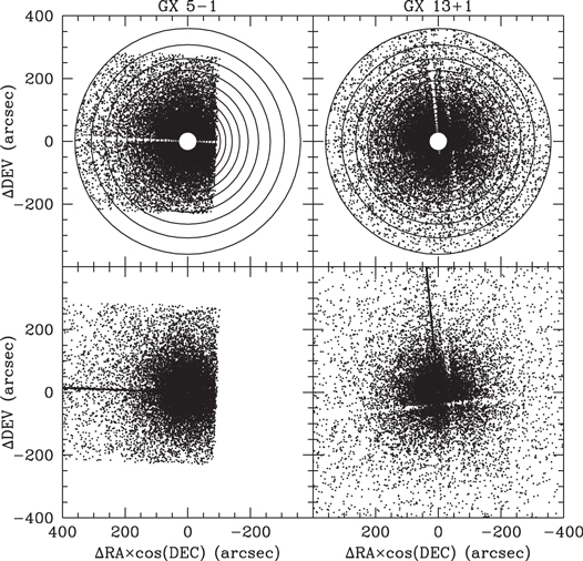
Figure 1. Maps of portions of the evt2 events with energies in the range 2–6 keV in the images of GX 5−1 and GX 13+1 before (bottom panels) and after (top panels) selection according to the criteria described in the text. Concentric circles in the top panels delineate the radial bins in which events were accumulated or the halo profiles.
Download figure:
Standard image High-resolution imageThe incident spectrum and flux of unscattered photons from each of the bright sources, required for the analysis and simulation of the halos, were derived from events in the ITS. During a main frame exposure (3.2 s for GX 5−1 and GX 13+1, and 3.1 s for Her X-1), extreme pileup of events in the CCD pixels located near the center of the focal plane image of a bright source precluded derivation of the required quantities from events near the center of the event image. Instead, they were derived from evt2 events within  of the center line of the ITS and farther than
  from the image center. Most of those events, which compose most of the ITS, are recorded by the same CCD pixels near the focal plane image center during the image transfers. But during the 0.04104 s of an image transfer, the charge content of every CCD pixel is shifted, row by row in 1024 steps, onto an adjacent storage CCD to form an event image for onboard processing and transmission as one frame of image data. The charge content of an image pixel that has swept through the center of the focal plane image during either the present or previous transfer consists of the charge accumulated during a main frame exposure at some distance from the image center plus the charge accumulated during its brief exposure near the image center. That exposure is approximately the time it takes for an image pixel to traverse the width of the PSF containing most of the unscattered photon flux, which is
  , equivalent to about 4 pw (1 CCD pixel width
  on the sky). Thus, the number of photon interactions that produced the charges carried by an image pixel on the center line of the ITS farther than
  from the image center is less by a factor of approximately
  than the number of photon interactions that produced the charges carried by an image pixel at the center of the image. The result is that the portion of the ITS farther than
  from the image center suffers only a small degree of pileup for which corrections were made as described in Appendix A.
The brevity of the time between charge shifts during an image transfer may effect the detection efficiency of the CCD pixels during the transfer. Lacking calibrated effective areas for analysis of ITS events, the effective areas for main frame events at the image center were used. To allow for errors in the derived photon fluxes that this may have caused, additional adjustable parameters were added to the halo-fitting process in the form of adjustable correction factors for the derived photon fluxes. The background of events in the ITS that were actually recorded during the main frame exposures was evaluated from the number of events in the angle range 8''–10'' from the center line, which included negligible portions of events recorded during image transfers. Cutoff correction factors for uncounted events in the ITS at angles greater than  from the center line are described in Appendix B.
For each quantity derived from the sum of N observed or simulated contributions  , a fractional statistical error σ was computed as
3. Properties of the Sources Derived from ITS
3.1. Light Curves
X-ray photons emitted at a given time, from a source at a distance of 8 kpc and scattered on their way to an observer, will arrive in a halo over a time range of ∼80 days owing to differences in their path lengths. Thus, flares and even day-to-day fluctuations of a given amplitude in the luminosity of a source cause much smaller or negligible fluctuations in the intensity of an observed halo. The top panels of Figure 2 display the average daily photon fluxes of GX 5−1 and GX 13+1 recorded by the All Sky Monitor (ASM) on the Rossi X-ray Timing Explorer during the 100 days before the Chandra observations. They show the day-to-day variations of the two sources. The middle panels display the numbers of events in  portions of the ITS per 30 image transfers (97.2 s) during the Chandra observations. The short-term fluctuations in the numbers of those events, which are produced primarily by unscattered photons, are larger than the Poisson errors, but much less in amplitude than the day-to-day fluctuations of the sources. The bottom panels display the numbers of predominantly halo events in the 30''–360'' radial range. Their fluctuations are slightly larger than Poisson, but much less in amplitude than the ITS fluctuations. Therefore, for the halo simulations described below, the photon fluxes and spectra of the sources were assumed to be constant and set to the average values derived from the ITS events.
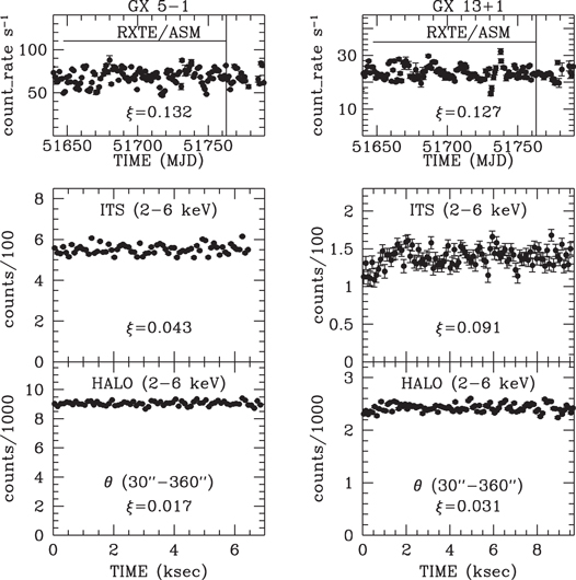
Figure 2. Top panels: light curves of GX 5−1 and GX 13+1 from the All Sky Monitor on the Rossi X-ray Timing Explorer. Each point is a 1-day average with its statistical uncertainty indicated. The horizontal lines indicate the intervals of 107 s during which most of the photons launched from a source at a distance of 8 kpc and scattered en route could have arrived in the observed halo. Middle panels: counts per 30 image transfers (96 s) of the unscattered photons derived from portions of the ITSs. Bottom panels: counts in 100 s intervals of photons in the halos of GX 5−1 and GX 13+1 in the angle range 30''–360''. The symbol ξ represents the rms deviation from the mean divided by the mean of the displayed rates.
Download figure:
Standard image High-resolution image3.2. Spectra
The spectra of GX 5−1 and GX 13+1 in the energy range 2–6 keV are plotted in Figure 3 as filled circles, each of which represents the background-subtracted photon flux Fj derived from ITS events of energy Ei in the jth energy interval between  , where
 ![${E}_{j}=[2.0+0.2(j-0.5)]$](https://content.cld.iop.org/journals/0004-637X/852/2/121/revision1/apjaaa1f0ieqn19.gif) keV,
keV,  , and
, and  . This was computed according to the formula
where  is the number of events in the angle interval 0''–2'' from the center line of the ITS and
  of its length,
  is the number of events in the angle interval 8''–10'', Aj is the effective area evaluated at the image center and averaged over the energy interval, Ts is the total exposure time of image transfers,
  is the fraction of the total length of the streak in which events were counted,
  is the pileup correction factor for events at distance di from the center line of the streak, and
  is the cutoff correction factor for the uncounted streak events in the angle range
  . Magnitudes of the correction factors are typically in the range 1.00–1.15 (see Appendices A and B).
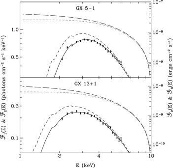
Figure 3. Model spectra fitted to the observed spectra of GX 5−1 and GX 13+1 derived from the ITSs. Left-hand scales: filled circles represent the observed values of the photon fluxes. Solid curves are plots of Equation (3) fitted to the data with the parameters listed in Table 2. Short-dashed curves are plots of Equation (4), which are the source spectra for trial photons. Right-hand scales: dotted curves are plots of Equation (5), which are the integrated energy fluxes from E to 10 keV of the unscattered photons. Long-dashed curves are plots of Equation (6), which are the integrated energy fluxes from E to 10 keV that would be received in the absence of any attenuation.
Download figure:
Standard image High-resolution imageIn each panel of Figure 3 the solid curve is a plot of the function
fitted to the measured quantities Fj by adjustment of the parameters  ,
,  , and
, and  to the values listed in Table 2. To avoid the degeneracy between photoelectric and scattering attenuation in the spectrum-fitting process, the total optical depth
  for scattering (henceforth "scattering depth") was fixed at 1.40, close to the values obtained as one of the variable parameters of the power-law dust models in the profile-fitting process described below. The photoelectric cross section of Morrison & McCammon (1983) was used for
  . The short-dashed curve is the function

which was the source spectrum from which the random energies were selected for the photons launched in the halo simulations. During the process of fitting a simulated halo profile to an observed halo profile, the total scattering depth  was among the variable parameters of the dust model. The dotted and the long-dashed curves are plots of the functions


which are, respectively, the energy flux of unscattered photons with energies in the range E–10 keV and the energy flux that would be received in the absence of any attenuation if  .
.
Table 2. Parameters of the Attenuated Exponential Functions Fitted to the Spectrum Data of GX 5−1 and GX 13+1
| Source |
 a
a
|
 b
b
|
 c
c
|
 d
d
|
 e
e
|
|---|---|---|---|---|---|
| GX 5−1 | 4.34 ± 0.01 | 2.80 ± 0.03 | 2.60 ± 0.01 | 1.40 | 3.94 |
| GX 13+1 | 1.55 ± 0.04 | 1.98 ± 0.06 | 2.13 ± 0.01 | 1.40 | 0.97 |
Notes.
aPhotons cm−2 s−1 keV−1. bH-atoms .
ckeV.
dFixed scattering depth for 1 keV photons.
eEnergy flux(1–10 keV) erg cm−2
.
ckeV.
dFixed scattering depth for 1 keV photons.
eEnergy flux(1–10 keV) erg cm−2  .
.
Download table as: ASCIITypeset image
If the intrinsic luminosities of the sources in the energy range 1–10 keV lie in the range  , where
  erg s−1 is the Eddington limit for a neutron star of mass
  , then the values of
  (1 keV) listed as
  in Table 2 imply that the distances of GX 5−1 and GX 13+1 lie in the ranges 1.9–6.0 kpc and 3.8–12.0 kpc, respectively.
4. X-Ray Halo Profiles
Each halo is characterized by its photon intensity Ijk in each of four equal energy intervals labeled by  in the range 2–6 keV and 16 annuli labeled by
  of equal logarithmic width in the range 30''–360'' from the source direction. The jth energy interval is between
  , where
  keV and
  . The kth annulus is between angles in arcseconds defined by
  , where
  and
and  . The quantity Ijk was computed according to the formula

where
Njk is the number of events in the jk energy-angle interval, T is the exposure time, Bj is the background intensity evaluated from events in the angle range 1067''–1247'', and  is the pileup correction factor for events at the angle
  from the image center (see Appendix A). The term
  , which represents the PSF multiplied by the unscattered photon flux, was estimated as
where  is the intensity profile of the Her X-1 image, and Fj and
  are the unscattered photon fluxes of the halo source and Her X-1, respectively, derived from events in their respective ITS. The quantity
  is the effective area solid angle of the kth angle interval in the jth energy interval. It was derived by numerical integration of the expression
where  is the solid angle of the kth annulus and (x, y) are the sky coordinates of its differential element. The error,
  , associated with Ijk is a combination of the statistical errors of Hjk and Bj, each computed according to Equation (1) and added in quadrature.
The normalized halo intensity profiles  of GX 5−1 and GX 13+1 are plotted in Figure 4, together with the raw image profiles, the PSFs, and the background levels. The solid curves are plots of six-degree polynomials fitted to the halo intensity profiles. The number in the lower left of each plot is the smallest quantity, which, added in quadrature to each of the fractional statistical errors of the 16 observed intensities, made the combined rms fractional deviations of the fitted polynomials from the observed intensities equal to or less than 1.0. The idea was to make the rms fractional deviations of the fit of a simulated halo profile not larger than 1.0 if the fit is as good as or better than that of the six-degree polynomial.
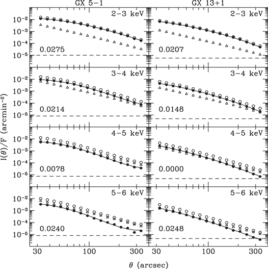
Figure 4. Radial intensity profiles (filled circles) of the X-ray halos of GX 5−1 and GX 13+1 divided by the unscattered photon fluxes derived from the ITSs. Each halo intensity profile was derived by subtracting the background (dashed line) and the PSF (open triangles) from the raw image intensity profile (open circles).
Download figure:
Standard image High-resolution imageThe differences between the profiles of the two halos, which presumably reflect differences between the spatial distributions of the dust along the two lines of sight, are more clearly displayed in Figure 5. In this and subsequent profile plots the plotted quantity is the normalized photon intensity multiplied by  .
.

Figure 5. Comparison of the halo intensity profiles of GX 5−1 and GX 13+1 divided in each case by the unscattered photon flux in the indicated energy range and multiplied by the square of the angle in arcseconds from the image center. The indicated errors include the errors added to make the rms fractional deviation of the fitted polynomial equal to or less than 1.0.
Download figure:
Standard image High-resolution image5. Halo Simulation Code
The simulation code is based on the theory of scattering of X-rays by small particles discussed by van de Hulst (1981), Mauche & Gorenstein (1986), and Mathis & Lee (1991). Calculations are carried out with small-angle approximations in a coordinate frame in which the source is at the origin, the z-axis is the line from source to observer, and z is the fraction of the distance from source to observer. A specified number n of trial photons are launched every second, beginning at a specified start time before the launch time of a photon that arrives without scattering at the start of the observation, and ending at the launch time of an unscattered photon that arrives at the specified end time of the observation. The photoelectric attenuation from source to observer is assumed to be the same for trial photons of a given energy that arrive in either the unscattered image or the halo. Accordingly, the energy of each trial photon is selected at random from the spectrum defined by Equation (4). Its path is tracked in three dimensions from scattering to scattering through a model of the dust. The distribution of the dust in space close to the z-axis is specified in the model by the quantity  such that the scattering depth for photons of energy E from source to a position (x, y, z) is
  . Dust grains are characterized by a single parameter a called size with a scattering cross section proportional to a4 (Mauche & Gorenstein 1986). Each trial photon, representing, in effect, a beam of many photons, is assigned a weight W equal to n times the integral of
  over the energy range 2–6 keV, which is the flux of real photons that would be observed in the absence of attenuation by scattering.
The depth of the first scattering and the corresponding value of z for each trial photon are selected from the distribution in scattering depth for photons of energy E. The emission direction is selected from a uniform distribution within a cone of directions with an opening angle equal to the maximum angle  from the line of sight that would allow the scattered photon to arrive before the end of the observation. At each scattering site the size of the dust grain from which the scattering occurred is selected from a distribution
  , where
  is the specified grain-size distribution. If a photon of energy E scattered by a grain of size a at the angle ϕ in the direction of the observer could arrive during the observation time, then the probability per unit solid angle of its going in that direction is computed in accordance with the Rayleigh–Gans approximation by the equation
where

The numerical factor in Equation (11) normalizes the total probability to unity. The contribution from a scattering to the simulated halo is computed as the product of several probability factors derived from each of the preceding random selections and attenuation between the scattering site and the observer. A new direction of the scattered trial photon is chosen at random from the same probability distribution. Contributions from additional scatterings, if they occur, are computed in the same way. Contributions from each number of scatterings are accumulated separately.
Details of the ray-tracing code and the Monte Carlo procedure were given in the previous publication (Clark 2004).1
As in the earlier study, the simulation code was validated by the close agreement between the simulated halo profiles for multiple scattered photons and the results derived analytically by Mathis & Lee (1991) for the case of 1 keV photons multiply scattered by a uniform distribution of spherical grains of radius  with a total scattering depth of 2 and a Gaussian approximation to the Rayleigh–Gans structure function.
6. Halo Simulations
The dust-scattered halo of a source with a given constant X-ray spectrum depends only on the physical characteristics of the dust and the dependence of its scattering depth on the fractional distance along the line of sight from source to observer. However, the earliest emission time of scattered trial photons that contribute significantly to a halo does depend on the actual distance of the source, which was set at an arbitrary 8 kpc. At that distance the start time for the simulations was set to 107 s before the emission time of unscattered trial photons that arrive at the start of observations. This proved to be early enough to ensure that all significant halo contributions were included.
Each dust grain model is specified by a distribution of the dust in space close to the line from source to observer and a distribution in size of the grains. The spatial distribution consists of a uniform density of dust with a total scattering thickness  plus 10 or fewer dust "clouds" characterized for the purposes of calculation as flat thin sheets perpendicular to the line of sight, the ith one of which extends from zi to
  with w = 0.001 and scattering thickness
  . The integrated scattering depth from the source to z along the line of sight is
Numerous grain-size distributions have been derived by various authors by fitting models of dust specified by composition to measurements of optical and infrared extinction. The three tested here are among those tested in the X-ray halo studies of Smith et al. (2006) and Smith (2008), namely, WD01 (Weingartner & Draine 2001), BARE-GR-B (Zubko et al. 2004), and MRN (Mathis et al. 1977). The last is a power law of the form  with
with  m,
m,  , and q = 3.5. In simulations with the power-law distribution both a2 and q were allowed to vary. Since the scattering cross section of spherical grains varies as a4, the probability distributions of the grains from which a scattering has occurred have the form
  as displayed in Figure 6.

Figure 6. Distributions in size of dust grains from which an X-ray photon has been scattered. PL designates power laws with values of q equal to 3.5 and 4.0; WD01 is for the favored distribution for graphite grains derived by Weingartner & Draine (2001); BARE-GR-B is a distribution for graphite grains derived by Zubko et al. (2004).
Download figure:
Standard image High-resolution imageEach halo simulation yields a set of photon intensities Sjk that are compared to the corresponding observed intensities Ijk. In fitting the simulated profiles to the observed profiles, the adjustable parameters of the dust model were one or more of zi,  ,
,  , and
, and  , plus a2 and q in fittings with the power-law grain-size distribution. Before the start of each step of the fitting process, the values of
  and
and  were multiplied by a common factor to make their sum equal to
  from the previous step. Also adjustable were the correction factors
  for the incident fluxes of unscattered photons derived from the ITS in the three energy intervals from 3 to 6 keV. The factor c1 was fixed at 1.0, so an error in the 2–3 keV photon flux would result primarily in compensating errors in the fitted scattering depths.
The deviation  between an observed and simulated intensity is defined as
where ![${\sigma }_{{jk}}={[{({\sigma }_{{jk}}^{h})}^{2}+{({\sigma }_{{jk}}^{s})}^{2}]}^{1/2}$](https://content.cld.iop.org/journals/0004-637X/852/2/121/revision1/apjaaa1f0ieqn88.gif) and
and  is the statistical error of Sjk. The computation seeks a set of model parameters that yields a minimum of the quantity
The quality of the fit for the four profiles is characterized by Q, and separately for each of the profiles by
The quantity Q, considered as a function of the parameters of the dust model, defines a hypersurface that is traversed by the Levenberg–Marquardt algorithm in search of a minimum. It has numerous potholes and flat valleys where the algorithm can halt before reaching the lowest minimum. In particular, every halting point of the fitting algorithm is in a nearly flat valley in which changes in  are compensated by changes in
  while
while  and Q remain nearly constant. However, the similarity of results obtained from numerous fittings with different initial conditions indicated that the fits reported here are close to the best attainable for the given dust models. Also, it should be noted that for a given rms difference between observed and simulated intensity profile, Q will increase as the number of events in the data increases and the resultant
  decreases. Since the number of events in the evt2 file for GX 5−1 is ∼1.8 times the number in the evt2 file for GX 13+1, the Q values for the GX 5−1 fits tend to be larger than those for the GX 13+1 fits.
The range of values of the contributions to a simulated halo was much wider than that of the contributions to an observed halo. Therefore, it was necessary to accumulate many more contributions to a simulated halo than the number of events of an observed halo in order to achieve statistical errors of Sjk substantially smaller than those of Ijk. To this end, the duration of the simulated observation was set to 107 s and the number of trial photons launched per second was set to 30, which yielded  contributions to each simulated halo. The code kept a record of the accumulated contributions to the simulated halo as a function of the launch time and the number of the multiple scatterings so that the validity of the start time could be checked after the simulation was completed.
Each set of trials with multicloud models began with 10 clouds plus a uniform density of dust between source and observer. In the fitting process the variable parameters were  and
and  with initial values of
  and zi with initial values of −0.05 + 0.1i, i = 1, 2, 3, ..., 10. In trials with the power-law size distribution, a1 was set to 0.005 μm, and a2 and q were variable with initial values of
  and 3.5, respectively. When two or more clouds were very close at the conclusion of a fitting, they were combined for a subsequent fitting with the aim of finding the set of model clouds that yielded the smallest attainable rms with the fewest clouds.
The fitting code was adapted to parallel computation of the numerous halo simulations required for numerical evaluation of the partial derivatives required for determination of the size and direction of each step in the process.
Results of the halo fittings are displayed in the top panels of Figures 7–18, in which the observed and simulated intensity profiles are plotted as filled and open circles, respectively. The deviations  are plotted below each profile panel. The dust model from which the simulation was derived is characterized by the three bottom panels: grain-size distribution (left), integrated scattering depth along the line from source to observer (middle), and integrated contributions of multiple scattered photons to the simulated halo plotted against time of emission relative to that of unscattered photons that arrive at the start of the observation (right).
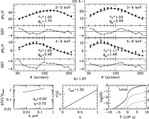
Figure 7. Halo profiles of GX 5−1 fitted by the profiles of a simulated halo generated with a uniform dust density and a power-law grain-size distribution.
Download figure:
Standard image High-resolution image
Figure 8. Halo profiles of GX 5−1 fitted by the profiles of a simulated halo generated with a uniform dust density and the WD01 grain-size distribution.
Download figure:
Standard image High-resolution image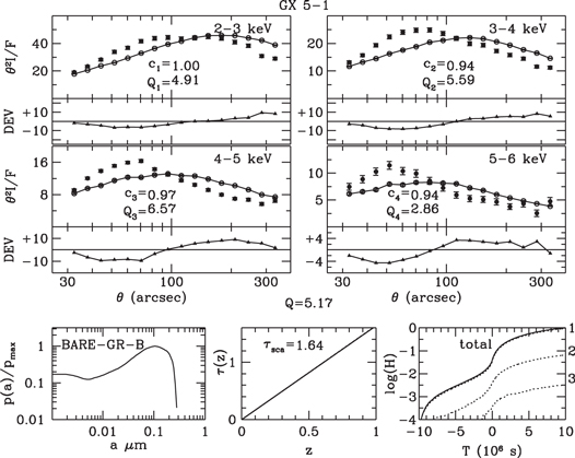
Figure 9. Halo profiles of GX 5−1 fitted by the profiles of a simulated halo generated with a uniform dust density and the BARE-GR-B grain-size distribution.
Download figure:
Standard image High-resolution image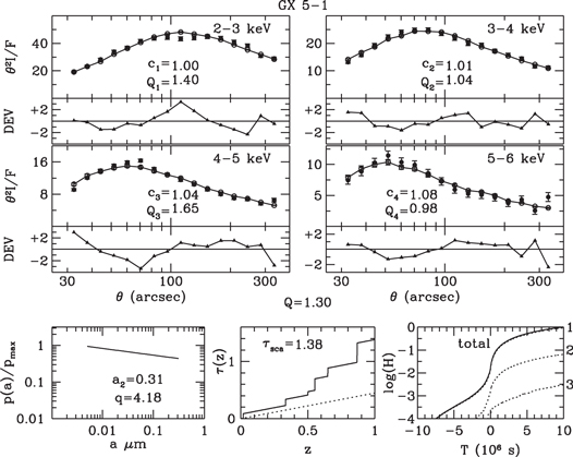
Figure 10. Halo profiles of GX 5−1 fitted by the profiles of a simulated halo generated with six dust clouds plus a uniform dust density and a power-law grain-size distribution.
Download figure:
Standard image High-resolution image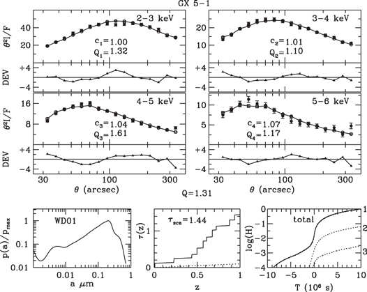
Figure 11. Halo profiles of GX 5−1 fitted by the profiles of a simulated halo generated with 10 dust clouds plus a uniform dust density and the WD01 grain-size distribution.
Download figure:
Standard image High-resolution image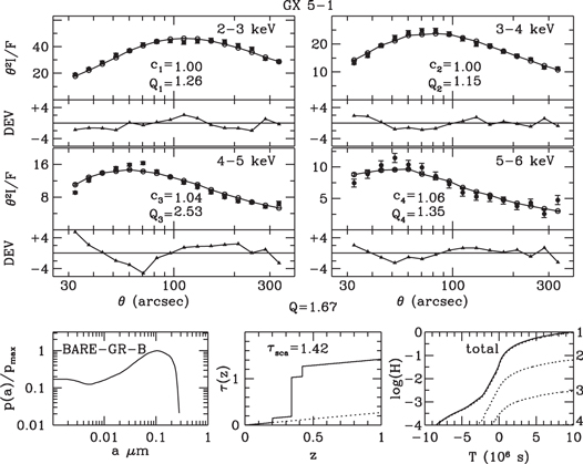
Figure 12. Halo profiles of GX 5−1 fitted by the profiles of a simulated halo generated with 10 dust clouds plus a uniform dust density and the BARE-GR-B grain-size distribution.
Download figure:
Standard image High-resolution image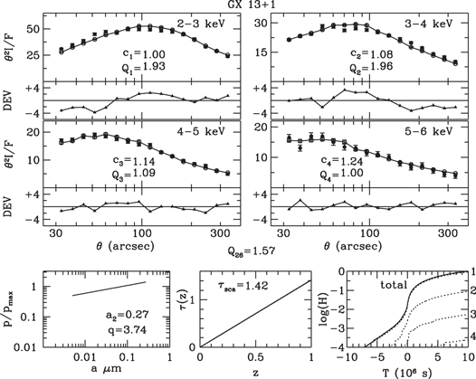
Figure 13. Halo profiles of GX 13+1 fitted by profiles of a simulated halo generated from a dust model with a uniform density and a power-law grain-size distribution.
Download figure:
Standard image High-resolution image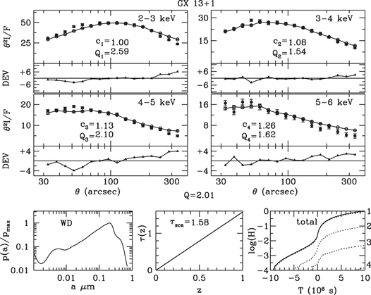
Figure 14. Halo profiles of GX 13+1 fitted by profiles of a simulated halo generated from a dust model with a uniform density and the WD01 grain-size distribution.
Download figure:
Standard image High-resolution image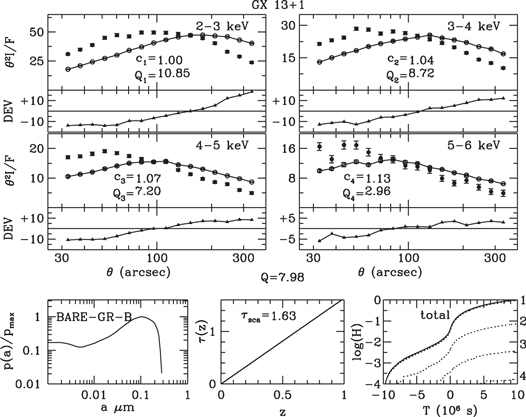
Figure 15. Halo profiles of GX 13+1 fitted by profiles of a simulated halo generated from a dust model with a uniform density and the BARE-GR-B grain-size distribution.
Download figure:
Standard image High-resolution image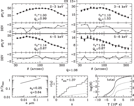
Figure 16. Halo profiles of GX 13+1 fitted by profiles of a simulated halo generated from a dust model with nine clouds plus a uniform density and a power-law grain-size distribution.
Download figure:
Standard image High-resolution image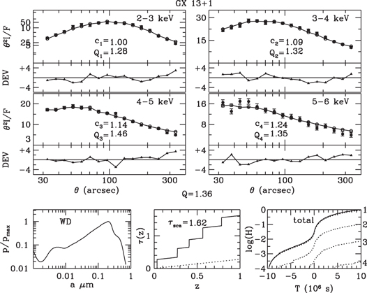
Figure 17. Halo profiles of GX 13+1 fitted by profiles of a simulated halo generated from a dust model with five clouds plus a uniform density and the WD01 grain-size distribution.
Download figure:
Standard image High-resolution image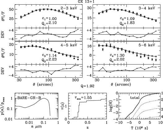
Figure 18. Halo profiles of GX 13+1 fitted by profiles of a simulated halo generated from a dust model with seven clouds plus a uniform density and the BARE-GR-B grain-size distribution.
Download figure:
Standard image High-resolution imageFigures 7–9 and 13–15 display the observed and fitted halo profiles of GX 5−1 and GX 13+1, respectively, for uniform spatial distributions and the three grain-size distributions. Results for multicloud models are displayed in Figures 10–12 and 16–18.
7. Discussion
The multicloud models of dust distribution employed in these simulations yielded consistently better fits to the observed halos of GX 5−1 and GX 13+1 than models with uniform spatial distributions, a result consistent with the well-known concentration of dust in molecular clouds and the naked-eye evidence of the dark clouds that obscure portions of the Milky Way. More significant is the fact that in nearly all the fitting trials, power-law grain-size distributions yielded substantially better fits than either the WD01 or BARE-GR-B distributions. The one exception is the multicloud WD01 fit of the GX 5−1 halo, for which the Q value is not significantly different from the Q value for the power-law fit. The fitted upper limits on grain size, a2, in the power-law distributions were close to that of the MRN distribution, but the fitted values of q were consistently larger than the value of 3.5 for the MRN distribution.
If a dust cloud in a simulation corresponds to a real discrete concentration of dust, and if its fractional distance to the X-ray source is accurate, then knowledge of the actual distance of the dust concentration will yield the distance of the source, and vice versa. Since both dust and CO are concentrated in molecular clouds, distance and content estimates of CO clouds, which can be derived from radio observations of the velocity spectra of CO, might provide clues to the actual distances of the dust clouds and the relative concentrations of CO and dust in molecular clouds. However, such distance estimates are highly uncertain because the radial velocity of a molecular cloud depends on the complex and uncertain structure and dynamics of the Galaxy and on its peculiar motion relative to the general galactic rotation. At the same time, the distances of GX 5−1 and GX 13+1 inferred from observations of their optical counterparts or from measurements of their X-ray brightness are also highly uncertain. Thus, it is not likely that a close correspondence will be found between the distances of CO concentrations derived from a velocity spectrum and the fractional distances of the dust clouds in a best-fit model. Moreover, infrared observations, particularly those of the Spitzer/GLIMPSE survey (Churchwell et al. 2009), show that at "resolutions  , interstellar dust is clearly distributed in fine, wispy filaments." Since the distribution of CO molecules within a molecular cloud must be more diffuse than that of the dust grains in such filaments, the correlation between measures of their abundance along any given line of sight is also not likely to be close.
Nevertheless, I explored the extent to which the best-fit dust models of the halo simulations might be related to features in the CO velocity spectra toward GX 5−1 and GX 13+1. The latter were kindly provided by T. M. Dame from the all-sky CO survey of Dame et al. (2001). Portions of those spectra, from  to
to  , are plotted as filled circles in Figure 19 as antenna temperature Ti against radial velocity Vi relative to the local standard of rest (LSR).
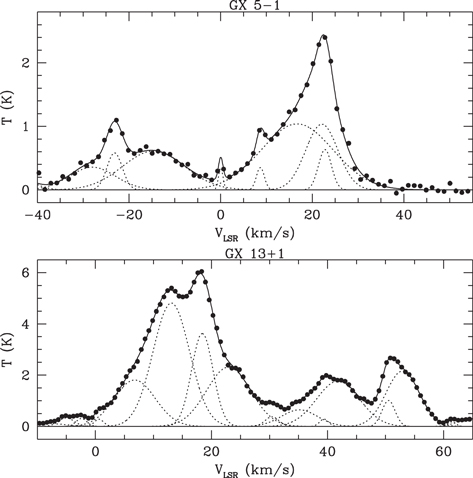
Figure 19. Portions of the velocity spectra of CO toward GX 5−1 and GX 13+1 (Dame et al. 2001). The filled circles are the measured antenna temperatures. In each case the dotted curves are Gaussians, the sum of which was fitted to the antenna temperatures and plotted as the solid curve. The fit was limited to the range of  corresponding to distances from the Galactic center greater than 3 kpc, which is the limit of the galactic rotation curve of Figure 13.
Download figure:
Standard image High-resolution imageI resolved the spectra into separate components corresponding to discrete concentrations of CO along a narrow line of sight by fitting each spectrum with a sum of Gaussians
in which the kth Gaussian represents a CO cloud with a peak antenna temperature Tk and a mean radial velocity Vk with a Gaussian spread Wk due primarily to turbulent motions within the molecular cloud.
In Figure 19 the component Gaussians are plotted as dotted curves and their sums as the solid curves. A quantity Ak, intended as a measure of the integrated density of CO through the kth cloud, was computed as
where  and
and  . The fitted values of the parameters are listed in Table 3. Assuming that the CO clouds with positive mean velocities move with the tangential velocity of galactic rotation, their distances were estimated according to the galactic rotation curve of Bobylev & Bajkova (2014), which is limited to distances from the Galactic center greater than 3 kpc. Figure 20 displays plots of the relations between distance D in the directions toward GX 5−1 and GX 13+1 and radial velocity VLSR relative to the local standard of rest of an object moving with the tangential velocity of the galactic rotation. The distances Dk listed in Table 3 were derived from Vk according to those relations.

Figure 20. Radial components of galactic rotation velocities in the directions of GX 5−1 and GX 13+1 plotted against distance according to the galactic rotation curve of Bobylev & Bajkova (2014).
Download figure:
Standard image High-resolution imageTable 3. Parameters of the Component Gaussians Fitted to the Velocity Spectra of CO Radio Emission in the Directions of GX 5−1 and GX 13+1
| Cloud No. | Tk(K) | Vk(km s−1) | Wk(km s−1) | Ak(K km s−1) | Dk(kpc) |
|---|---|---|---|---|---|
| GX 5−1 | |||||
| 1 | 0.36 | −27.99 | 5.02 | 4.48 | ⋯ |
| 2 | 0.58 | −23.14 | 1.68 | 2.44 | ⋯ |
| †3 | 0.61 | −14.63 | 6.76 | 10.34 | 1.00* |
| †4 | 0.35 | 0.02 | 0.49 | 0.42 | 0.01 |
| †5 | 0.35 | 8.67 | 0.86 | 0.76 | 2.41 |
| †6 | 1.04 | 16.70 | 7.84 | 20.40 | 4.10 |
| 7 | 1.03 | 22.09 | 3.51 | 9.10 | 5.09 |
| 8 | ⋯ | ⋯ | ⋯ | 8.93 | 5.10* |
| 9 | 0.63 | 22.77 | 1.42 | 2.26 | 5.21 |
| GX 13+1 | |||||
| 1 | 0.14 | −10.06 | 4.08 | 1.21 | ⋯ |
| 2 | 0.33 | −5.01 | 1.36 | 1.13 | ⋯ |
| 3 | 0.31 | −2.41 | 0.93 | 0.72 | ⋯ |
| 4 | 0.28 | 0.61 | 0.82 | 0.57 | 0.08 |
| †5 | 1.81 | 6.78 | 3.52 | 15.99 | 0.84 |
| †6 | 4.81 | 13.09 | 3.16 | 38.10 | 1.53 |
| †7 | 3.62 | 18.42 | 1.85 | 16.82 | 2.07 |
| †8 | 2.31 | 22.95 | 3.79 | 22.00 | 2.50 |
| †9 | 0.38 | 30.43 | 1.19 | 1.13 | 3.17 |
| †10 | 0.65 | 35.15 | 3.11 | 5.05 | 3.57 |
| 11 | 0.28 | 39.39 | 0.78 | 0.56 | 3.93 |
| †12 | 1.77 | 41.81 | 3.70 | 16.39 | 4.12 |
| †13 | 1.01 | 50.51 | 1.12 | 2.85 | 4.82 |
| †14 | 2.16 | 52.95 | 2.86 | 15.53 | 5.01 |
Download table as: ASCIITypeset image
In the CO spectrum toward GX 5−1 the features with negative velocities clearly cannot be attributed to clouds actually moving with the local tangential velocity of galactic rotation. Smith et al. (2006) attribute all of the CO with negative velocities to the expanding 3 kpc arm of the Galaxy located at an estimated distance of 5.1 kpc with a large component of velocity in a direction away from the Galactic center. However, if the features displayed as dotted curves at negative velocities in Figure 19 correspond to actual distinct CO clouds, then it may be more plausible to attribute clouds 1 and 2 in Table 3 to a single turbulent cloud in the 3 kpc expanding arm and cloud 3 to a separate closer cloud with a peculiar radial component of velocity. Accordingly, clouds 1 and 2 are listed as a single cloud 8 at a hypothetical distance of 5.1 kpc with a total value of A equal to the sum of their A values, and cloud 3 is assigned a hypothetical distance of 1.0 kpc.
Possible correlation between dust and CO cloud distances are displayed in Figures 21(a) and (b). In this figure each CO cloud is represented by a horizontal line with an ordinate equal to its distance Dk. The corresponding value of Ak is at the left end of each line. Each slant line is a plot of the implied distance Di of the ith dust cloud at fractional distance  against the assumed distance D of the X-ray source. The scattering depth
  of the dust cloud is at the right end of its slant line. The horizontal dashed line below the plot shows the range of possible distances cited in Section 3.2. The slant and horizontal lines terminate at radial distances where the distance from the center of the Galaxy is 3 kpc.
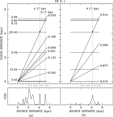
Figure 21. Correlations between the distance estimates of CO clouds derived from the velocity spectrum of CO in the direction of GX 5−1 and the fractional distances of dust clouds in models fitted to the profiles of the GX 5−1 halo. Left panels: for the best-fit dust model (Figure 10). Right panels: for the dust model (Figure 22) biased in favor of the CO cloud distances and a source distance of 4.17 kpc.
Download figure:
Standard image High-resolution imageIf every dust cloud coincided with a CO cloud and every distance and fractional distance were without error, then every slant line would cross a horizontal line at the same source distance, indicating a perfect correlation. As a measure of the actual degree of correlation, a quantity C(D), defined by the equation
is plotted in the bottom panel. In this equation  and
and  are the numbers of dust clouds and CO clouds, respectively. If the correlation function had a maximum at a plausible source distance D, then the plausibility of that distance was tested by determining whether or not the profiles of a simulated halo, derived from a dust model with clouds at distances close to the estimated distances of the CO clouds, can be fitted to the observed profiles with a low value of Q. The items in Table 3 marked with an asterisk were used in those tests.
The correlation function in Figure 21(a) is for the best-fit dust model in Figure 10. It shows several maxima that indicate possible choices for an estimate of the source distance D. To test the plausibility of a given value of D, I set the initial parameters of a dust model to be  ,
,  ,
,  , and
, and  , where i and k are the indices of CO clouds closer than D. A first fitting was done with zi fixed and
  adjustable. A second fitting was then done with the final parameters from the first fitting as initial parameters and zi added to the adjustable parameters.
The correlation maximum at  in Figure 21(a) is close to where a slant line crosses the horizontal lines of CO clouds 7 and 8 of Table 3 and close to where two other slant lines cross the horizontal line of CO cloud 5. The plausibility test for this value of D yielded a six-cloud fit with Q = 1.381, but with the correlation maximum shifted to a distance of 5.35 kpc, at which four of the slant lines crossed close to horizontal lines.
A source distance of 4.17 kpc at the position of the other plausible correlation maximum leaves four clouds for the plausibility test. It yielded the fitted profiles displayed in Figure 22 and the correlation plot in Figure 21(b). The Q value of 1.376 is slightly less but not significantly better than Q for the distance of 5.35 kpc. But the fact that the fitting process yielded a simulated halo with a nearly exact correlation of dust and CO cloud distances for a source distance of 4.17 kpc may indicate that 4.17 kpc is a more plausible value for the distance of GX 5−1. At that distance the implied 1–10 keV luminosity of GX 5−1 would be  erg s−1.
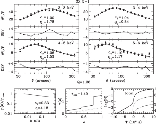
Figure 22. Halo profiles of GX 5−1 fitted in two stages by profiles of a simulated halo generated from a dust model biased in favor of the CO cloud distances with four dust clouds plus a uniform density and a power-law grain-size distribution.
Download figure:
Standard image High-resolution imageThe same analysis was applied to the dust and CO clouds toward GX 13+1. The correlation plot for the best-fit nine-cloud dust model and the CO cloud distances listed in Table 3 is displayed in Figure 23(a). A source distance of 5.60 kpc at the position of a minor peak in the correlation function offers the possibility of close or near coincidences between nine dust and nine CO clouds. With an initial dust model derived from nine CO cloud distances and the trial source distance of 5.60 kpc, two fittings, the first with fractional distances fixed and the second with variable fractional distances, yielded the fit with Q = 1.18 displayed in Figure 24 and the correlation plot displayed in Figure 23(b). At 5.60 kpc the implied 1–10 keV luminosity of GX 13+1 would be  erg s−1.
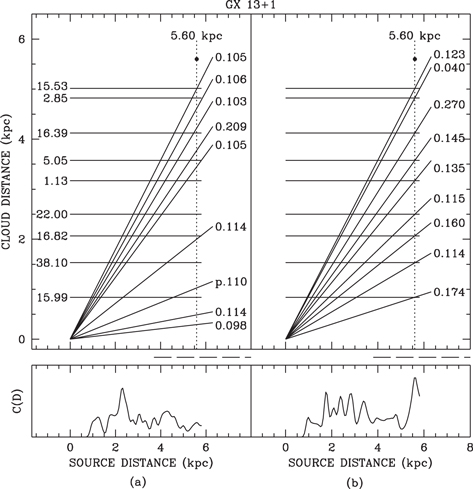
Figure 23. Correlations between the distance estimates of CO clouds derived from the velocity spectrum of CO in the direction of GX 13+1 and the fractional distances of dust clouds in models fitted to the profiles of the observed GX 13+1 halo. Left panels: for the best-fit dust model (Figure 16). Right panels: for the dust model (Figure 24) biased in favor of the CO cloud distances and a source distance of 5.60 kpc.
Download figure:
Standard image High-resolution image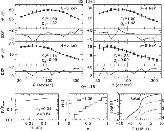
Figure 24. Halo profiles of GX 13+1 fitted in two stages by profiles of a simulated halo generated from a biased dust model with nine clouds plus a uniform density and a power-law grain-size distribution.
Download figure:
Standard image High-resolution imageIn spite of the apparent success in fitting the profiles of simulated halos generated from dust models derived from the multi-Gaussian CO cloud models, there is an obvious problem with the wide range of the ratios  . Some relatively small part of that range can be attributed to errors. But the question remains as to whether or not the concentration of dust in "wispy filaments," referred to above, is sufficient to account for so wide a range in the ratios of dust to CO densities along the lines of sight to the sources.
Finally, I note that the flux correction factors ci increased monotonically with energy in all of the GX 13+1 and most of the GX 5−1 halo simulations. A flux value determines the rate at which trial photons are launched in a simulation. If it is undervalued, the resulting shortfall in the simulated halo profile intensity is automatically compensated during the fitting process by an increase in the flux correction factor. Flux values were derived from events in the ITS that were analyzed with effective areas calibrated for the long exposures. The upward trend of ci indicates that the detection efficiency of the ACIS CCDs during rapid image transfers decreases with energy relative to the values expressed by the calibrated effective areas. And since the correction factor c1 was fixed at 1.0 during the fittings, the trend indicates that the uncorrected flux values for the energy range 2–3 keV may have been underestimated and compensated by positive errors in the fitted values of the scattering depths.
The GX 5−1 events were recorded on back-side-illuminated (BI) CCDs, the GX 13+1 events on front-side-illuminated (FI) CCDs. Thus, the wider range of the flux correction factors in the GX 13+1 halo fittings indicates that the decrease in detection efficiency for ITS events might be greater in the FI CCDs than in the BI CCDs.
8. Conclusions
- 1.Multicloud models of the spatial distribution of interstellar dust yield simulations of the X-ray halos of GX 5−1 and GX 13+1 that fit observed halo profiles better than uniform distributions.
- 2.Power-law grain-size distributions with exponents near 4.0 yield better fits than either the WD01 or BARE-GR-B distributions.
- 3.The scattering depth for X-rays with in the range 2−6 keV in the best-fitting dust models for both GX 5−1 and GX 13+1 is close to .
- 4.Evidence for correlation between the dust and CO clouds in the direction of GX 5−1 is consistent with the source being located at a distance of 4.17 kpc with an implied 1–10 keV luminosity of erg s−1.
- 5.Evidence of correlation between dust and CO clouds toward GX 13+1 indicates a likely distance of 5.6 kpc and a 1–10 keV luminosity of erg s−1.
- 6.The increase with photon energy of the flux correction factors indicates that the detection efficiency of the ACIS CCDs for events recorded during rapid image transfers decreases with energy relative to the efficiency during long exposures.


The MIT-Kavli Center for Astrophysics and Space Research provided the facilities for this work. Kenton Phillips, Omri Schwartz, Paul Hsi, and Isaac Meister provided essential assistance in the use of the center's computer systems. Mark Bautz advised me on properties of the ACIS and the data system of the Chandra observatory. I thank T. M. Dame for providing the CO data. I am especially grateful to Alan Levine for a careful reading and critique of a draft of this paper.
This research made use of data obtained from the Chandra Data Archive and software provided by the Chandra X-ray Center (CXC).
Appendix A: Pileup Corrections
Each frame of data transferred from an ACIS CCD to temporary storage is automatically searched on board for events defined as a 3 × 3 pixel array with an induced charge above threshold in the center pixel larger than that in any of the surrounding eight (Chandra Teams 2015). Some events, e.g., those caused by a hot pixel, are automatically rejected on board. The rest are assigned grades 0–7 according to the pattern of charges in the array and transmitted to ground for processing, which places in an evt1 file its grade, transmission time, energy, and the celestial arrival direction of its incident photon relative to a fixed point in the sky. Events with grades 0, 2, 3, 4, and 6 are selected for an evt2 data file, for which calibration in the form of "effective areas" and other data are provided.
When two or more charge patterns produced in the same exposure frame overlap, the resulting pileup may yield no event in the evt1 file, or one or more events with erroneous grades and energies. Since the effect can occur at any level of incident photon intensity, accurate image analysis must be limited to regions where the effect of pileup on intensity estimates is either negligible or small enough to allow plausible correction.
Figure 25 shows the effect of pileup on the image profiles of GX 5−1, GX 13+1, and Her X-1. In each case the density of events in the evt1 file per data frame is zero at the center owing to extreme pileup and reaches a maximum value less than ∼0.2 arcsec−2 frame−1 at an angular distance in the range 2''–8''. The effects of pileup in causing erroneous grade assignments in evt2 data are displayed in Figure 26, where relative frequencies of grade 0, 2, and 6 events are plotted separately against angle from the image center. The plots change rapidly with angle as the densities of events decrease, until they reach nearly flat plateaus, where the effect of pileup on grade determinations is small.
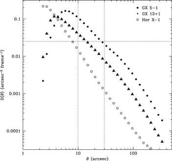
Figure 25. Average density of evt1 events per data frame plotted against angular distance from the image center for each of GX 5−1, GX 13+1, and Her X-1. Dotted vertical lines indicate the lower limits of the angular ranges in which intensity profiles were derived with corrections for small degrees of pileup.
Download figure:
Standard image High-resolution image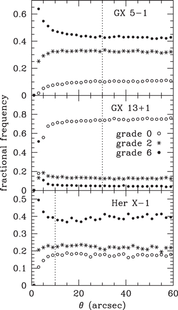
Figure 26. Relative frequencies of G026 events with energies in the range 2–6 keV plotted against distance from the image centers of GX 5−1, GX 13+1, and Her X-1.
Download figure:
Standard image High-resolution imageThe first step in estimating pileup corrections was a compilation, frame by frame, of the separations between evt2 events and all evt1 events in the same frame over the angle range of interest. The resulting numbers in the range of separations 0–8 pw for the three bright sources are displayed as histograms in the panels of column A in Figure 27. The numbers are zero for separations less than 1 pw, are small from 1 to 2.2 pw, and increase beyond 2.2 pw with large fluctuations that reflect the discrete set of distances between CCD pixel centers. The same analysis was performed on scrambled data in which each event in the evt1 file was exchanged with another selected at random from the entire file, thereby destroying the intraframe positional correlations. The results are displayed in the panels of column B. The numbers increase with separation as before, but without the large fluctuations and, in particular, without the losses in the 0–2.2 pw range due to pileup. The ratio in column C of a column A histogram to the corresponding column B histogram is a measure of the probability that a photon that strikes a CCD will yield an evt2 event as a function of the separation between it and other photon strikes in the same data frame. In column D are plots of a quantity I call the detection efficiency  , which is the same ratio as that plotted in column C for
  pw but 1.0 for
  pw.
pw.
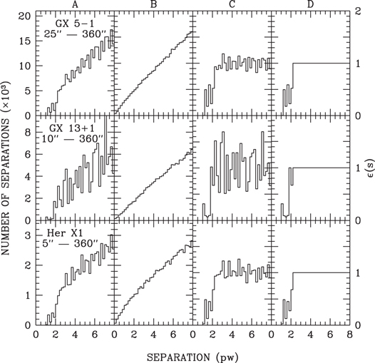
Figure 27. Column A: number of separations between each evt2 event in the energy range 2–6 keV and all evt1 events in the indicated angle ranges from the image centers, compiled frame by frame and plotted against the separation. Column B: same as column A, except the data were scrambled as explained in the text. Column C: ratio of column A number to column B number plotted against separation. Column D: functions  plotted against s and employed as the detection efficiency in the pileup simulations.
Download figure:
Standard image High-resolution imageThe next step was an iterative process that yielded a set of factors by which the intensity profiles derived in this study were corrected for pileup. The process generated many frames of pseudo-data, each one with a total number of candidate events equal to a Poisson variate of the average number of real evt1 events per frame in the angle range of the profile to be corrected, and distributed in angle at random in proportion to the observed radial intensity profile and at random in azimuth. For each event its separation s from each of the others in the same frame was computed and its survival as a candidate was determined with a probability equal to  . The profile of the surviving candidate events was computed, and for each radial bin the ratio between the intensity of the generating profile and the survival profile was the first approximation to the pileup correction factor for that bin. The generating profile for the next iteration was computed as the previous generating profile multiplied by the correction factors. Five iterations proved sufficient to achieve convergence to a set of correction factors.
The resulting sets of pileup correction factors for Her X-1, GX 5−1, and GX 13+1 and their effects on the radial profiles of evt1 events are displayed in Figure 28. The same correction factors were applied to all radial intensity profiles derived from evt2 events.
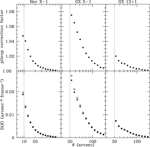
Figure 28. Bottom panels: per-frame density profiles of all events in the evt1 data files before (filled circles) and after (open circles) pileup corrections. Top panels: ratios of corrected to uncorrected event densities.
Download figure:
Standard image High-resolution imageA similar process was employed to derive pileup correction factors for the lateral intensity profiles of the ITS used in deriving the spectra of the unscattered photons of GX 5−1, GX 13+1, and Her X-1. The results are summarized in Figure 29.
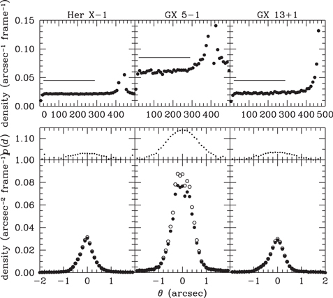
Figure 29. Top panels: longitudinal density profiles of all evt1 events in the ITS within  of the center line of the streak plotted against the angular distances from the edges of the CCD chips. The horizontal bars indicate the portions of the streaks from which the lateral profiles were compiled. Middle panels: pileup correction factors. Bottom panels: lateral density profiles of events in the evt1 data files of Her X-1, GX 5−1, and GX 13+1 plotted against the angular distance from the center line of the ITS. The filled and open circles represent the profiles before and after application of the pileup correction factors, respectively.
Download figure:
Standard image High-resolution imageAppendix B: Streak Cutoff Corrections
The spectra and fluxes of unscattered incident photons were derived from events in the ITS within  of its center line and over the length of the center line indicated by the horizontal line in the top panels of Figure 29. Background events, mostly accumulated during the main frame exposures, were assessed from events between
  and
and  . The correction factors for the uncounted ITS events beyond
  were derived from estimates of the SSF, which was derived, in turn, from estimates of the PSF in the angular range 0''–1000'' from the image center.
B.1. Point-spread Functions
I call  the PSF at the angular distance θ from the image center for the jth energy interval. It was assembled in three sections from observations of the point sources with negligible dust-scattered halos listed in Table 4. The section for 0''–1
 5 was derived from the sum of images of seven faint quasars, the section for 15–10'' from the sum of three images of PKS 2155–304, and the section for 10''–360'' from one image of Her X-1. The final result of stitching the three sections together is expressed by the following equations:
Table 4. Point-like Sources with Chandra Images Used for Evaluations of the PSF and SSF of the ACIS
| Object | OBS_ID |

|
|---|---|---|
| Faint Quasars 0''–15 |
||
| PKS B1345+125 | 836 | +71 |
| PG 1634+70 | 1269 | +37 |
| PKS 2201+044 | 2960 | −38 |
| *PKS 0458−02 | 2985 | −25 |
| *PG 2112+05 | 3011 | −28 |
| PKS 2316−423 | 3972 | −65 |
| *PKS 0208−512 | 4813 | −62 |
| Bright Quasar 15–10'' |
||
| PKS 2155−304 | 1014 | −51 |
| 1705 | −51 | |
| 3167 | −51 | |
| Binary Pulsar 10''–720'' | ||
| Her X-1 | 3662 | +38 |
Note. An asterisk indicates that the source has a jet excluded in the analysis.
Download table as: ASCIITypeset image
The coefficients ai and bi are listed in Table 5. They yield unit flux over the angular range 0''–1000'', which required extrapolation of Equation (21) beyond the angle limit of data for the Her X-1 profiles. The purpose of the extrapolation was to reduce the error in the cutoff correction derived from the estimate of the SSF caused by the high-angle cutoff of the PSF. Plots of  against θ for the four energy intervals are displayed in Figure 30.
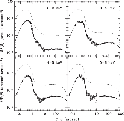
Figure 30. PSFs (solid lines) and SSFs (dotted lines) of the ACIS derived from the image profiles of seven faint quasars (filled circles), PKS 2155–304 (open circles), and Her X-1 (filled triangles). For display the PSF and SSF are multiplied by  and θ, respectively.
Download figure:
Standard image High-resolution imageTable 5.
Coefficients of the Functions (Equations (20) and (21)) Fitted to the Normalized PSFs in the Angular Range 01–1000'' Derived from the Image Profiles of Seven Faint Quasars, the Bright Quasar PKS 2155–314, and Her X-1
| Coefficient | 2–3 keV | 3–4 keV | 4–5 keV | 5–6 keV |
|---|---|---|---|---|
| a1 | 0.2625 × 10+1 | 0.2688 × 10+1 | 0.1923 × 10+1 | 0.1674 × 10+1 |
| a2 | 0.1598 × 10+0 | 0.1614 × 10+0 | 0.1818 × 10+0 | 0.2128 × 10+0 |
| a3 | 0.2994 × 10+1 | 0.2925 × 10+1 | 0.2962 × 10+1 | 0.3286 × 10+1 |
| a4 | 0.5564 × 10+0 | 0.3706 × 10+0 | 0.4533 × 10+0 | 0.4126 × 10+0 |
| a5 | 0.5143 × 10+0 | 0.5528 × 10+0 | 0.5330 × 10+0 | 0.5450 × 10+0 |
| b1 | −0.1918 × 10+1 | −0.1834 × 10+1 | −0.1655 × 10+1 | −0.1966 × 10+1 |
| b2 | −0.3055 × 10+1 | −0.2971 × 10+1 | −0.4790 × 10+1 | −0.3327 × 10+1 |
| b3 | −0.3622 × 10+0 | −0.1418 × 10+0 | 0.3060 × 10+1 | 0.1377 × 10+1 |
| b4 | 0.8642 × 10+0 | 0.7515 × 10+0 | −0.1402 × 10+1 | −0.5421 × 10+0 |
| b5 | −0.3464 × 10+0 | −0.3438 × 10+0 | 0.2912 × 10+0 | 0.6881 × 10⁻¹ |
| b6 | 0.4125 × 10⁻¹ | 0.4459 × 10⁻¹ | −0.2418 × 10⁻¹ | 0.3652 × 10⁻³ |
Download table as: ASCIITypeset image
B.2. SSFs and Cutoff Corrections
SSFs were derived from the corresponding PSFs by a Monte Carlo process that generated 107 random values of θ with a frequency distribution  . Each generated angle was multiplied by
  , where ϕ was a random value between 0 and π. The product, representing the angular distances
  of a simulated event from the center line of the ITS, were counted in angle bins from
  to
to  . Each count was divided by the total number of generated counts to obtain a value of
  at the midpoint
  of the ith bin. The SSFs are displayed as dotted curves in Figure 30.
The fractions of events included and excluded within a radius in the image of a point source were computed, as functions of the angular limit θ on the events counted by integrating the PSFs from 0'' to θ and from θ to 1000'', respectively. The results are plotted as the solid curves in Figure 31. The included and excluded fractions for the SSFs were similarly computed as functions of the limiting angle from the center line of the ITS, and the results are plotted as dotted lines in Figure 31. In each plot a vertical line is drawn at 2'' to its intersection, with the dotted line representing the fraction of events excluded by limiting the count to the angle range 0''–2''. That fraction and the corresponding correction factor Cj for the intensity of unscattered X-rays derived from such a count are printed above and below the intersecting horizontal line, respectively. A cubic spline was applied to the four values of cj to obtain the nine values fitted and displayed in Figure 32.
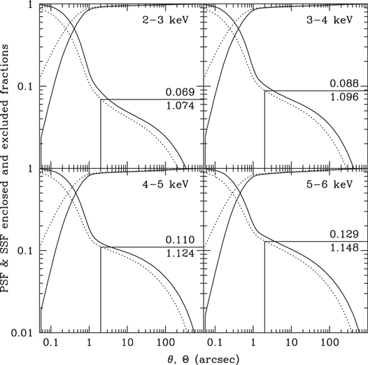
Figure 31. Integrated PSFs and SSFs of the ACIS for four energy intervals from 2 to 6 keV. Solid lines represent the fraction of events in the image of a point source enclosed and excluded within an area bounded by a circle concentric with the image center plotted as a function of the radius of the circle. Dotted lines represent the fraction of events in the transfer streak of a point source enclosed or excluded within an area bounded by lines parallel to the ITS plotted as a function of the distance of the bounding lines from the center line of the ITS. In each panel the number above the horizontal solid line is the fraction of ITS events excluded for a bounding distance of  , and the number below is the corresponding average cutoff correction factor for events in the indicated energy range.
Download figure:
Standard image High-resolution image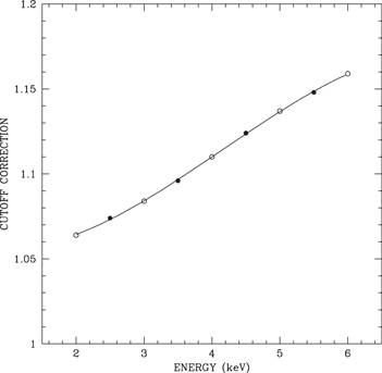
Figure 32. Cutoff correction plotted against energy for intensities derived from events within  of the center line of the ITS. Filled circles are the values indicated in Figure 31; open circles are derived by a spline interpolation and extrapolation.
Download figure:
Standard image High-resolution imageFootnotes
- 1
Equation (A19) of that publication should be