
Abstract
Continuous observations of temporal variations in the Earth's gravity field have recently become available at an unprecedented resolution of a few hundreds of kilometers. The gravity field is a product of the Earth's mass distribution, and these data—provided by the satellites of the Gravity Recovery And Climate Experiment (GRACE)—can be used to study the exchange of mass both within the Earth and at its surface. Since the launch of the mission in 2002, GRACE data has evolved from being an experimental measurement needing validation from ground truth, to a respected tool for Earth scientists representing a fixed bound on the total change and is now an important tool to help unravel the complex dynamics of the Earth system and climate change. In this review, we present the mission concept and its theoretical background, discuss the data and give an overview of the major advances GRACE has provided in Earth science, with a focus on hydrology, solid Earth sciences, glaciology and oceanography.
Export citation and abstract BibTeX RIS
Invited by Mike Bevis
1. Introduction
Gravity is one of nature's fundamental forces. Although most people tend to think of gravity—or, more precisely, the gravitational acceleration g at the Earth's surface—as a constant of approximately 9.81 m s−2, it is not uniform around the globe. The Earth's rotation and its equatorial bulge cause deviations from the mean value of about half a percent, which can be well predicted from theory. Because the Earth's gravity field is a product of its mass distribution, variations in the density of the Earth's interior and topography cause further regional deviations of a few tens of a millionth of g (figure 1). These are much harder to model, since this requires knowledge of the Earth's structure. However, mass transport in the interior is a slow process, so that these deviations can be considered to be more or less constant on human timescales. Water, on the other hand, is much more mobile than rock and its constant movement on the Earth's surface and in the atmosphere will cause changes in the gravity field on a wide range of time scales. These variations are minute, but measuring them accurately means literally 'weighing' changes in the Earth's water cycle and could help unravel the complex dynamics of the Earth system and climate change. The list of possible applications of time-variable gravity measurements is abundant: tracking changes in the water held in the major river basins, observing variations in the hydrological cycle, measuring the ice loss of glaciers and ice sheets, quantifying the component of sea level change due to transfer of water between the continents and oceans, detection of water droughts and the depletion of large groundwater aquifers due to unsustainable irrigation policies, and much more, would all be possible. And even processes within the solid Earth would be measurable, provided that they occur fast enough and their gravitational signal is strong enough (e.g., mega-thrust earthquakes). As we will see, all of this and more has become reality at a global scale since the launch of the Gravity Recovery And Climate Experiment (GRACE) satellites.

Figure 1. Static gravity anomalies based on 4 years of GRACE observations, illustrating the regional variations in the gravity field due to topography and variations in the Earth's density. The anomalies are computed as the difference between gravity on the geoid and the normal gravity on a reference ellipsoid. Units are milligal (1 mGal = 10−5 m s−2).
Download figure:
Standard image High-resolution imageAlthough the temporal gravity variations associated with the phenomena listed above are extremely small (∼10−8 m s−2), they can be measured with dedicated instruments. Locally, time variations in gravity can be recorded accurately on the ground by gravimeters [1], but global, satellite-based, measurements of time-variable gravity have long been restricted to mapping large-scale variations only. These early observations were mainly based on satellite laser ranging (SLR), which involves measuring the position of satellites orbiting the Earth, with a precision of a few cm or better. Such a high precision is obtained by emitting a laser pulse to a dedicated satellite, covered with reflectors, and measuring the round-trip travel-time once the reflected pulse is received. By collecting a sufficient amount of such position measurements, the orbit can then be determined, which is for a large part determined by the Earth's gravity field. However, these satellites—such as the Laser Geodynamics Satellites (LAGEOS [2]), launched in the 1970s and 1990s and still operational today—orbit the Earth at a high altitude (∼6000 km) to minimize atmospheric drag. Because the sensitivity to the Earth's gravity field decreases with increasing altitude, the determination of time-variable gravity with SLR is restricted to scales of typically 10 000 km (e.g., [3]). For a higher resolution, satellites at a lower altitude are required, such as the Challenging Minisatellite Payload (CHAMP; [4]) satellite, which allowed continental-scale gravity observations at seasonal periods (2000–2010), and in particular GRACE, the subject of this review article.
Like many space missions, GRACE had a long history of negotiation and deliberation before the satellites saw daylight. For at least two decades prior to its launch, the Earth Science community had been calling for a dedicated gravity satellite mission to provide an improved determination of the Earth's static, global gravity field (e.g., [5–8]). While that message had always been well received by NASA and other space agencies, the arguments had not been persuasive enough to lead to an approved mission. A combination of events in the late 1990s changed that situation, and culminated in the acceptance of GRACE. One was the innovative GRACE measurement concept itself, which permits the recovery of monthly global gravity solutions of unprecedented accuracy down to scales of a few hundred km. Originally, though, the focus of GRACE was still to be on the static field. But officials at NASA, wondering about the possible scientific payoff of time-variable gravity measurements, commissioned the US National Research Council to undertake a study to look into this. Prior to that study, it was known that a mission like GRACE could recover the secular gravity changes due to vertical land motion to a useful accuracy, but there had been virtually no work done on the possible use of time-variable satellite gravity to study other processes. The resulting NRC committee, chaired by Jean Dickey, discovered a multitude of possible applications that were well suited to the expected spatial and temporal resolution of GRACE [9]. The proposed GRACE mission design and science plan were subsequently adjusted to focus on the time-variable field, rather than on the static field. The usefulness of these time-variable applications and their relevance to such a wide variety of Earth science disciplines, as well as the perceived ability of GRACE to recover those signals, were certainly among the factors that influenced the decision by NASA and DLR, the German space agency, to fund the mission. Relatively soon after funding was approved, the mission was launched on March 17, 2002, from Plesetsk Cosmodrome in Russia.
GRACE has lead to important new insights in many scientific fields, ranging from verifying the 'Lense–Thirring effect' of general relativity [10] to the detection of a giant meteorite impact crater underneath the Antarctic ice sheet [11], to observing tropospheric density changes during geomagnetic storms [12], but it has greatly advanced our understanding of how masses move within and between the Earth's subsystems (land, ocean, ice and the solid earth, in particular [13, 14]). Before reviewing the progress made in time-variable gravity research since the launch of GRACE, we briefly discuss the mission design, some essential equations and the GRACE data.
1.1. The GRACE satellites & data
Although every satellite mission is a mammoth, complex operation, the basic principle of GRACE is beautiful in its simplicity. GRACE consists of two satellites in a low, near-circular, near-polar orbit with an inclination of 89°, at an altitude of about 500 km, separated from each other by a distance of roughly 220 km along-track (figure 2). The mission does not measure gravity directly with an active sensor, but is based on the satellite-to-satellite tracking concept, which tracks variations in the intersatellite distance and its derivatives to recover gravitational information. Suppose the satellites approach a sizeable mass located on the Earth's surface (e.g., an ice sheet): since the two GRACE satellites are separated by a certain distance, and the gravitational pull of the mass is inversely proportional to the squared distance to each satellite, the orbit of each of the satellites will be perturbed slightly differently. The leading satellite will be pulled slightly more toward the mass than the trailing one and the separation between the satellites will increase. Although these changes are minute—in the order of a few micrometers, or 1/100th of the width of a human hair—they can be measured by means of a dual-one way ranging system, the K/Ka band microwave ranging system (KBR). Non-gravitational forces, such as atmospheric drag will also alter the relative distance, and are accounted for using onboard accelerometer measurements. The orientation in space of the satellites are mapped by two star-cameras. Since the KBR measurements provide no information on the position in the orbit, the satellites are equipped with Global Positioning System (GPS) receivers so that their location is known.

Figure 2. Artist's impression of the GRACE satellites (credit: NASA).
Download figure:
Standard image High-resolution imageFrom these data, called the level-1 data, variations in the Earth's gravity field can be recovered. This is generally done through an iterative procedure: first, an a priori model of the Earth's mean (static) gravity field in combination with other 'background' force models (e.g., representing luni-solar and third body tides, ocean tides, the pole tide, etc) is used to determine the orbit of both satellites. Importantly, the gravitational effects of ocean and atmosphere mass variations are removed from the measurements at this step using numerical models, because otherwise their high-frequency contributions would alias into longer periods and bias the results. Next, this predicted orbit is compared to the GPS and KBR observations and residuals are computed. Linearized regression equations are constructed, which relate the gravity field (more specifically, the spherical harmonic coefficients as we will see next) and other parameters to the residuals and are used to update the orbit. By combining data of a sufficiently long period—about a month, which guarantees a sufficient ground track coverage of the satellites—these equations can be used to relate the level-1 observations to variations of the gravity field in a least square sense (see [15, 16]). The GRACE data are processed at three main science data centers, i.e., the Center for Space Research (CSR) and the Jet Propulsion Laboratory (JPL), both located in the USA., and the German Research Centre for Geosciences (GFZ) in Germany. Differences in the approaches of the processing centers lie in the background models used, the period over which the orbits are integrated, weighting of the data, the maximum degree of the estimated gravity harmonics, etc [17–19]. Other institutes are also providing independent gravity solutions nowadays, often based on alternative approaches (see, e.g., [20–22]).
Next, we discuss the basic equations behind temporal gravity and the GRACE data. For the casual reader, it suffices to know the GRACE data generally are distributed as (Stokes) coefficients of spherical harmonic functions of degree l and order m, which can be related to variations in water height at the Earth's surface. The maximum harmonic degree of the data depends on the analysis center, but in all cases it is sufficient to provide a spatial resolution of roughly 300 km.
The Earth's gravitational field is described by the geopotential V. At a point above the Earth's surface, with spherical coordinates radius r, co-latitude θ and longitude λ, it can be expressed as a sum of Legendre functions:

where G is the gravitational constant, M the mass of the Earth and ae denotes its mean equatorial radius. Plm are the Legendre polynomials of degree l and order m, and Clm and Slm are the spherical harmonic coefficients. The higher the order l, the smaller the spatial scale (see, e.g., [23], for a good introduction). Note that as l increases, (ae/r)l+1, and consequently variations in V become smaller. Thus, satellites at lower altitudes r can better resolve small wavelength features.
Equation (1) may be used to define equipotential surfaces, i.e. surfaces of constant potential V. The equipotential surface that would best fit the mean sea level at rest is referred to as the geoid, which in turn can be approximated by an ellipsoid of rotation. The height difference between such a 'reference ellipsoid' and the geoid is referred to as the geoid height and is approximated by Bruns formula:

where U is the gravitational potential on the reference ellipsoid, equal to the constant potential of the geoid, and γ the normal gravity on the ellipsoid's surface. The latter can be further approximated by
 , so that in turn the geoid height can be approximated by [23]:

From this it follows that variations in the geoid height can be fully described by the spherical harmonic coefficients Clm and Slm, referred to as Stokes coefficients in geodesy. It is this set of coefficients that is estimated from the satellite measurements and distributed by the GRACE science teams every month as level-2 data. The maximum degree l of the monthly Stokes coefficients lies between 60–120, which corresponds to a spatial resolution of roughly 150–300 km (20 000 km/l).
Geoid height is a commonly used unit in geodesy, but one more step is required to relate the Stokes coefficients to changes in (water) mass distribution, a more intuitive metric to most researchers studying the Earth's water cycle. On monthly to yearly time-scales, changes in the Earth's gravity field are primarily caused by redistribution of water in its fluid envelope, which all take place within a thin layer of a few kilometers near the Earth's surface. In this case, (ae/r)l+1 in equation (1) reduces to 1 and the anomaly in surface density (i.e., mass per area) can then be obtained using the following equation (see [24], for a step-by-step derivation):

where we included the symbol Δ to indicate that we are dealing with time-variable quantities, and ρe is the average density of the Earth (5517 kg m−3). The load Love numbers k'l (e.g., [25]) account for deformation of the solid Earth due to the loading of the mass anomaly on its surface, which will cause a small gravity perturbation as well. Units of Δσ are typically kg m−2. Often, the surface density is divided by the density of water, which yields surface water height in meters water equivalent. An example of the surface height anomaly observed by GRACE for August 2005 is shown in figure 3. When integrating Δσ over an area, one obtains a volume estimate, usually expressed as km3 of water, or, equivalently, gigatonnes (Gt). One gigatonne equals 1012 kg, a sea level rise of 1 mm requires approximately 360 Gt of water.

Figure 3. Maps of the observed surface water height anomaly for August 2005, based on three GRACE releases: (a) the original first release (CSR RL01); (b) the fourth release (CSR RL04) and (c) fifth release (RL05). The data are smoothed with a 350 km Gaussian kernel.
Download figure:
Standard image High-resolution imageThe monthly GRACE Stokes harmonics are publicly available and can be downloaded from http://podaac.jpl.nasa.govpodaac.jpl.nasa.gov and http://isdc.gfz-potsdam.de. While the availability of GRACE data only as unfamiliar spherical harmonics originally slowed its application toward wider use by non-geodesists, the data has more recently been made available in easier-to-use gridded format as well (http://geoid.colorado.edu/grace/grace.php or http://grace.jpl.grace.jpl.nasa.gov/data/). Yet, as we will see later on, interpretation of these gridded maps is not always straightforward and requires some expertise.
Some researchers also derive regional mass anomalies directly from the level-1 range-rate data. In a method originally developed to study the gravity field of the moon, point masses or regional uniform mass concentrations ('mascons') are spread over the Earth's surface. The gravitation acceleration exerted by each mascon is then expressed as a sum of spherical harmonic functions so that the effect on the GRACE orbit can easily be computed. Each mascon is then given a scaling factor which is adjusted to give the best fit to the regional KBR observations (e.g., [26, 27]). Although this approach is computationally much more demanding, it has certain advantages, e.g., regional solutions can be obtained and certain constraints can be applied between neighboring mascons to reduce the leakage problem, as discussed below.
1.2. Handling the GRACE data
The first GRACE science results were published about two years after the mission launch [28, 29]. Many geophysical features—such as the seasonal change in water storage in the Amazon river system—were readily recognizable, but surprisingly, the maps of surface water height showed distinctive North–South striping patterns (figure 3(a)). Although it had been anticipated during the mission design phase that the higher degree Stokes coefficients (i.e., small spatial scale) would have larger errors than the lower degrees (large spatial scale), such—clearly unphysical—striping had not been foreseen. The origin of these stripes lies in the orbit geometry of the GRACE mission (e.g. [30, 31]). The gravity field is sampled using the variations in the along-track distance between the two satellites, which circle the Earth in a near-polar orbit. As a result, the observations bear a high sensitivity in the North–South direction, but little in the East–West direction. Errors in the instrument data, shortcomings in the background models used to remove high-frequency atmosphere and ocean signals, and other processing errors will consequently tend to end up in the East–West gravity gradients. Since the release of the first GRACE data, methods to process the satellite data have improved and new ocean and atmosphere models allow for a better removal of high-frequency variability signals from the observations. This has led to new, reprocessed GRACE solutions, which contain significantly less noise than earlier releases [32], as illustrated in figure 3. Yet, although much reduced, the North–South striping problem persists.
Several methods have been developed to reduce the effect of noise in the GRACE data. One technique converts the global spherical harmonics into a local time series and then averages the observations over a larger, pre-determined region, such as river or drainage basins. If the area is sufficiently large—larger than the spatial decorrelation scale of the noise—the noise will tend to cancel out. Based on this concept, [33] formulated a 'basin averaging approach' which aims to isolate the signal of individual regions while minimizing the effects of the noise and contamination of signals from the exterior. The 'basin averaged' time series of the surface water anomalies can then be analyzed or compared to regional ground-based measurements. This has become a very common method of analysis with GRACE, especially in hydrological studies (see section 2).
Another straightforward and very commonly applied approach reduces the noise in the GRACE observations by smoothing the data. In the spectral domain, this means weighting the Stokes coefficients depending on the degree l, with a lower weight given to the noisier, higher degree Stokes coefficients. In the spatial domain, this is equivalent to convolving the GRACE maps with a smoothing kernel. A popular kernel is the Gaussian, bell-shaped, function, which decreases smoothly from unity at its center to zero at large angular distances (figure 4) and is characterized by its smoothing radius, i.e., the distance on the Earth's surface at which the kernel value has decreased to half the value at its center [24, 34]. As the smoothing radius increases, the higher degree Stokes coefficients are damped more strongly and the noise in the GRACE data is reduced (figures 5(a)–(c)). Unfortunately, using a large smoothing radius also means that the true, geophysical signals are damped and are smeared out over large regions, hindering a straightforward interpretation of the GRACE observations.

Figure 4. Value of a Gaussian smoothing kernel W for a smoothing radius of 500 km, (a) as a function of the distance from the center point and (b) as a function of the spherical harmonic degree l.
Download figure:
Standard image High-resolution image
Figure 5. Surface water height anomaly for August 2005 observed by GRACE (based on CSR RL05 data), smoothed with a Gaussian kernel with three different smoothing radii: (a) 0 km; (b) 200 km and (c) 500 km. An animation showing the 500 km monthly surface water height anomalies for 2003–2012 is available from the online supplementary data (stacks.iop.org/RoPP/77/116801/mmedia).
Download figure:
Standard image High-resolution imageThe Gaussian kernel has an isotropic character, i.e., it is independent of orientation, but as discussed above, the noise in the GRACE data has a strong non-isotropic North–South character. Non-isotropic filters have been developed [35, 36], but these generally still require a large smoothing radius to remove all stripes in the GRACE maps. A closer inspection of the GRACE Stokes coefficients by Swenson and Wahr [37] revealed that striping patterns could be traced back to correlated errors in the Stokes coefficients of even and odd degree l, respectively. This opened the door to more advanced post-processing methods which allowed a further increase of the spatial resolution of the GRACE data. To reduce the intercoefficient correlation, Swenson and Wahr [37] fit a quadratic polynomial in a moving window to the Stokes coefficients of even and odd degrees separately (for a fixed order m) and removed this from the original Stokes coefficients. Other methods apply principal component analysis on the Stokes coefficients [38] or use the full variance–covariance matrix of the Stokes coefficients [39, 40] to decorrelate the GRACE solutions. These advanced post-processing methods have lead to a reduction of noise in the GRACE data of 50% and more (figure 6; [41]).

Figure 6. Surface water height anomaly for August 2005, smoothed with a 200 km Gaussian kernel as in figure 5(b), but now with the destriping algorithm of Swenson and Wahr [37] applied.
Download figure:
Standard image High-resolution imageUnfortunately, the limited resolution of the GRACE data and the required post-processing means that the observations do not represent point-measurements. Additionally, any type of post-processing filter or during-processing constraint which reduces GRACE errors can also reduce local signal amplitude [42–45]. So, when studying a specific region, one cannot simply take the average of the GRACE observations over that region. Besides the signal attenuation, leakage effects will bias such a simple average: due to the low resolution, water mass variations in neighboring areas will spill into the desired region, while part of the signal of interest will spread outside the region. Leakage is particularly problematic in regions of high spatial variability in surface water storage patterns, as well as along coastlines where smoothing with the ocean's far smaller signal notably damps the apparent hydrological signal. Rescaling is commonly used to remedy the signal loss caused by post-processing and the transformation of point-source signals to a finite number of spherical harmonics (e.g., up to degree and order 60). To compute a rescaling parameter, a model is made with higher spatial resolution than GRACE, then transformed to the limited set of spherical harmonics that GRACE uses and post-processed identically to GRACE. A ratio of the original model to the post-processed model signal amplitude is called the rescaling parameter. Assuming that the model reasonably represents the spatial pattern of the true signal, this ratio can act as a multiplier to upscale or downscale the actual post-processed GRACE data and counter the amplitude damping effect seen as leakage. Typically, the rescaling has been done on a basin scale (e.g., [46]), though recently Landerer and Swenson [44] have tested and released a 1° × 1° mapped version of GRACE with rescaling and rescaling errors included, specifically focused at hydrologists. Nonetheless, limitations and inaccuracies at short spatial scales remain a problem, especially as the focus moves to smaller and smaller basins.
In addition to spatial limitations, GRACE's typical monthly sampling rate also limits its ability to estimate signals that act at shorter than seasonal time scales, though it handles annual and longer-term signals well. Recently, a few sub-monthly signals have been produced [20, 26, 47–50], but the remaining delay between observation and data delivery makes real-time assessments (for which they would be most desired) impossible. Typically, increasing the temporal resolution of the GRACE time series means accepting an increased noise level in the signal, since the ground track coverage becomes less dense. Various types of constraints can ameliorate the difficulty, but not eliminate it entirely—and these constraints often alter the signal strength along with that of the noise.
After these introductory sections, we will now give an overview of the Earth Science applications of GRACE in the fields which have most benefited from this unique new set of time-variable gravity observations (hydrology, solid Earth sciences, glaciology and oceanography). Each section discusses the unknowns before GRACE was launched, the major scientific advances the mission provided and its limitations.
2. GRACE and hydrology: a bound on terrestrial water storage
GRACE's ability to accurately measure sub-yearly to decadal-trend mass changes on the global and regional scales has made it a unique data source for hydrology and hydrological modeling. Prior to the GRACE mission, total terrestrial water storage (TWS) changes over land could not be measured over significant spatial or temporal scales. Instead, the focus was on individual pieces of TWS: groundwater (GW), near-surface and deep soil moisture (SM), surface water (SW), snow-water equivalent (SWE) and ice, and water contained within biomass (BIO). These subsections of the terrestrial water storage were measured via in situ systems or other satellites, and/or were modeled from basic principles. However, the difficulty and expense of establishing and maintaining reliable in situ observation systems is significant, especially over large and remote areas and for long periods of time. Where observation coverage is good, in situ measurements have focused on particular sub-sections of the water signal, resulting in, for example, excellent coverage of near-surface SM and GW, but no knowledge at all of SW. Hydrological models also reflect this, often lacking one or more components of water storage in their computations. A growing selection of remote sensing hydrologic tools exist, but few have long data records and none besides GRACE see signals below a shallow subsurface layer.
GRACE's ability to measure the sum of all hydrologic components in the water column, over the entire planet, at monthly intervals has proven a bounty for large-scale hydrological researchers. Two parallel techniques exist when using GRACE for hydrologic purposes. The first, as suggested above, is to solve for changes in TWS directly, based on changes (Δ) in some or all of the individual components of water storage listed above:

This technique is particularly valuable in combination with observed data for some of the terms on the right-hand side of equation (5), using GRACE to give the ΔTWS sum. The second common technique is to consider the processes which cause changes in terrestrial water storage, principally precipitation (P), evapotranspiration (E) and runoff/discharge (R):

This is often useful for modelers, who can use GRACE's estimate of terrestrial water storage changes to bound their estimates of P, E and/or R, oftentimes in combination with other observations of those same variables. The combination of P − E can also be estimated based on atmospheric anomalies, if the change in water vapor and the divergence of the atmospheric moisture transport are known. Whether using equation (5) or (6), GRACE measurements present a mathematical bound which did not exist before.
Besides the main limitations of GRACE mentioned in the introduction, such as the need for smoothing and post-processing, the limited spatial resolution and leakage of GRACE signal into and out of the desired region, a major complexity with using GRACE for hydrologic purposes is inherent in its definition: GRACE measures the entire water column as one measurement. This makes separation into hydrologic constituents complicated, requiring combination with other hydrologic products, all of which have their own limitations and errors. The differing spatial and temporal scales between GRACE (a global, monthly product) and in situ data such as river or well gauges (point-source measurements which are non-uniform in space and time) makes exact comparisons and combinations difficult. Complications can also arise if non-hydrologic mass signals, such as alterations of mass in the atmosphere or solid Earth or leakage from the nearby ocean, also occur in the region, a particular problem given that models to correct for such signals are not perfect. The lower noise levels of GRACE RL05 [32] are expected to reduce many of these problems, but the general design of the GRACE mission means that they cannot be completely eliminated.
The use of GRACE by hydrologists has gone through two historical stages: validation and full utilization. For several years after the 2002 launch of GRACE, the focus was on using hydrological models and observational data to determine the accuracy of GRACE itself. Many of the initial comparisons were qualitative and large-scale. Various researchers [26–28, 51] created side-by-side comparisons of GRACE with hydrological models, as in figure 7(a), or otherwise noted that the dynamically active regions seen by GRACE matched where hydrological models and our previous understanding of weather and climate placed them. Others [29, 52, 53] compared GRACE results to hydrological models across large basins (figure 7(b)) and noted that both amplitude and phase were typically close. Later, EOF analyses were used to better quantify the similarities [54, 55]. The images shown here use the most recent CSR RL05 GRACE series from February 2004 to January 2012, but even one or two years of RL01 GRACE were sufficient to verify the general accuracy of GRACE in large, hydrologically active regions.

Figure 7. Comparison of (a) annual signal amplitude and (b) signals across three large basins for CSR RL05 GRACE and the hydrology models GLDAS and WGHM. Data is from 2004–2011, 300 km Gaussian smoothing applied to all series.
Download figure:
Standard image High-resolution imageOnce several years of GRACE data had been garnered, hydrological GRACE papers became more in-depth and quantitative, using models, in situ data, or both to verify the general accuracy of GRACE and estimate the combined error in GRACE and their other data sources. A fine early example is Swenson et al [56], who made use of a widespread in situ well and SM network in the US state of Illinois. Based on prior knowledge, they assumed that the dominant terms in equation (5) in Illinois were GW and near-surface SM, ignoring SW, snow, and the effect of the biosphere. They smoothed and destriped three years (2003–2005) of GRACE RL01 data, took the significant gravitational signal associated with vertical land motion (see section 3) into account, then used a basin average to compute the ΔTWS time series over the Illinois region. When they compared the GRACE ΔTWS to the sum of in situ ΔSM and ΔGW from wells, they found good agreement (figure 8(a)). Seasonal amplitudes ranged between 5–10 cm depending on the year, while the RMS difference from the in situ ΔGW + ΔSM was only 2 cm, much of which was likely caused by the 1.8 cm in estimated GRACE RMS errors. The three-year correlation between ΔTWS from GRACE and ΔGW + ΔSM from in situ measurements was 0.95. This was put forth as early evidence that seasonal hydrological signals seen by GRACE are reasonable. Additionally, Swenson et al found that in Illinois, SM and GW are of approximately equal magnitude, with soil moisture sometimes lagging the GW by a month or two (figure 8(b)). This means that in order to compare with GRACE, estimates of both GW and soil moisture are needed, not merely one or the other, a finding which has been confirmed via terrestrial gravity measurements (e.g., [57]). Thus a model which ignores either one would be unable to represent the true terrestrial water storage well.

Figure 8. (a) Total water storage anomalies from GRACE in the Illinois region (circles are monthly anomalies, gray line is the data smoothed to accentuate the seasonal variations), and combined in situ SM and GW measurements (black line is the smoothed time series). X-axis is time in years, and Y-axis is storage change in mm. (b) In situ SM and GW storage anomalies. Circles are monthly anomalies of SM to 1 meter depth, triangles are GW anomalies below 1 meter depth; gray/black lines are smoothed soil moisture/GW smoothed time series respectively. Adapted from [56] with permission of John Wiley & Sons, Inc. Copyright 2006 by the American Geophysical Union.
Download figure:
Standard image High-resolution imageUnfortunately, GW is not predicted by several global hydrology models, including one of the more commonly used: the Global Land Data Assimilation System (GLDAS, [58]). Moreover, it proved difficult to find other in situ systems of measurement for both GW and SM over large areas. Rodell et al [59] worked around this in the greater Mississippi basin by combining what they did have: in situ well measurements for GW, and SM and SWE estimates modeled by GLDAS. Rather than combining the in situ ΔGW with the modeled ΔSM + ΔSWE and comparing to GRACE's ΔTWS, they worked equation (5) backward, solving for the ΔGW which the GLDAS model could not provide. They compared that to the in situ well measurements—which are not available in many areas of the world—for verification that ΔGW can be estimated in such a manner. Using two years of RL01 GRACE data (2002–2004), they demonstrated that the seasonal GW signal in the wider Mississippi basin can be estimated using GRACE terrestrial water storage and the SM+SWE from a model. However, when they repeated the same procedure for smaller subbasins of the Mississippi, they found that the technique failed to properly determine the seasonal well signal in basins smaller than about 900 000 km2. While well undersampling in the spatial domain and inaccurate assessments of well specific yields also provided serious concerns, the dominant error source in these smaller subbasins was assumed to be the RL01 GRACE product.
A similar study was performed across the US state of Oklahoma [60], and another over the High Plains Aquifer in the US [61]. The latter is particularly interesting in that it investigated water storage changes in a semi-arid region which is heavily irrigated using GW. It thereby touched on the socio-economic issue of water scarcity and large-scale human pumping for GW, something not considered by most large-scale hydrological models at the time. Strassberg et al [61] averaged the RL01 GRACE fields into three-month seasons to better reduce noise, then compared to in situ GW data from 2719 intermittent wells in the area and modeled soil moisture estimates from NLDAS (North American Land Data Assimilation System). The GW and SM signals were both large (5–7 cm maxima) and varied differently in time, with a clear seasonal signal in the GW but not in the SM. They found a correlation of 0.82 between GRACE ΔTWS and the ΔGW + ΔSM combination from the wells and model (above the 95% confidence level). A 3.3 cm RMS difference existed between the two series, largely caused by a greater estimated amplitude of ΔGW + ΔSM compared to GRACE, which Strassberg et al [61] posited may be due to overestimation of ΔGW during local summer, when irrigation pumping is occurring. Despite the imperfect matching, this paper provided firm evidence that GRACE could add value to hydrological studies even in semi-arid regions where significant GW was being pumped for irrigation.
Even before the launch of GRACE, hydrological modelers were aware of imperfections in their models due to missing terrestrial water storage components. However, these errors of omission came into sharp relief when presented with independent GRACE results. For example, numerous researchers noted that while the spatial pattern of GRACE ΔTWS matched with models, the amplitude of the models was notably lower in many high-signal locations than what was seen with GRACE (the Amazon basin in figure 7, for example) and occasionally differed slightly in phase as well (the Ganges basin in figure 7). As the GRACE timespan lengthened, interannual variations and long-term slopes (figure 9) were also found to differ locally [54, 62, 63]. Based on comparisons like those listed above, modelers began to trust GRACE more and started considering GRACE during their cycles of model improvements, to better tune their parameters [64, 65] or directly assimilate GRACE TWS into their models [66, 67].

Figure 9. Comparison of trends in SW height for CSR RL05 GRACE (top) and the hydrology models GLDAS (middle) and WGHM (bottom). Data is from 2004–2011, 300 km Gaussian smoothing applied to all series.
Download figure:
Standard image High-resolution imageNiu and Yang [68] wrote one of the earliest examples demonstrating GRACE's use in improving hydrology models. They began with the standard NCAR CLM hydrology model and, based on in situ information and basic principles, altered it in five significant ways: (1) decreasing the canopy interception of precipitation, (2) altering the percolation rate through the soil column, (3) decreasing surface runoff and thus increasing infiltration of the surface, (4) reducing the rate of subsurface flow, and (5) increasing the permeability of frozen soil. These modifications were made ahead of time, then compared to GRACE, along with the original CLM model, as verification. They found that the alterations resulted in ΔTWS maps which more closely matched what GRACE saw than the original series did, demonstrably increasing the amplitude of the hydrology signal in high-signal areas like the Amazon and Zambezi basins. When looked at as basin-wide averages, the RMS difference between the modified model time series and GRACE was half or less the size of the RMS difference between the original model and GRACE over large cold basins (Ob), classic monsoon basins (Yangtze), and tropical rainforest basins (Amazon). The improvement continued to hold for basins on the order of 300 000 km2, as well. This demonstrated not simply an improvement of one model over another, but also a method with which the independent GRACE data set could help determine the precise features of a model which cause improvement. In a later paper, Niu et al [69] used similar techniques to determine an appropriate runoff decay factor for use with modeled snow.
Werth and Güntner [65] used GRACE to tune the WaterGAP Global Hydrology Model (WGHM) in a more statistically rigorous fashion. As they had only six years of GRACE data (2003–2008), they removed all long-term trends and focused only on seasonal and interannual variability. They performed sensitivity analysis on 21 model parameters having to do with SM, GW, SW, SWE and BIO over 28 large river basins. After choosing the 6–8 most sensitive parameters in each separate basin, they used a Pareto-based multi-objective calibration scheme to balance the fit to GRACE's ΔTWS and a secondary independent data set, river discharge. Their optimized results were then compared to the original model and explanations given for the differences seen. Overall, the calibrated model increased the variability of terrestrial water storage throughout the tropical and temperate regions while decreasing it in colder areas, making the calibrated model better match what is seen with GRACE. The parameters causing the changes depended largely on the basin. In tropical and temperate basins, a deeper rooting depth allowed for greater seasonal storage as SM. In basins with widespread rivers, lower river flow velocities and larger runoff coefficients kept water in the rivers for longer, thus increasing and delaying the seasonal maxima in terrestrial water storage. In colder basins, raising the temperature of snow melt drove the snow to melt later, changing the phase of the signal more than the amplitude. GW variability decreased in many arid and semi-arid regions due to increased evapotranspiration. The optimization findings also suggested a route forward to more improvements, such as using more than one SM layer to prevent excessive drying from evaporation, decorrelating the soil moisture from GW in some areas, and testing to optimize parameters which set GW timing and river volume. Werth and Güntner [65] noted that while a few basins were relatively insensitive to this optimization scheme, in general, the use of GRACE in combination with river discharge rates improved the tuning of the WGHM.
A similar combined optimization scheme using river discharge and GRACE TWS was also used by Lo et al [64] to tune their CLM model, and Zaitchik et al [67] assimilated the two data sets along with GW observations into their GLDAS model for testing as well. Houborg et al [70] assimilated GRACE into the Catchment Land Surface Model (CLSM), then applied that model to the specific problem of drought monitoring in North America. They first determined that the GRACE-assimilated model better matched in situ GW+SM data than did the original, un-assimilated CLSM model in most areas of the US. The addition of GRACE helped overcome various weaknesses in the CLSM, while the assimilation technique allowed the individual terrestrial water storage components of surface SM, root-zone soil moisture, and GW to be separated (figure 10), as they cannot be in GRACE alone. This combination of GRACE plus model could help improve the US and North American Drought Monitors in the future.

Figure 10. Correspondence between (a) the GRACE monthly water storage anomaly fields, (b) the US Drought Monitor product, and (c) drought indicators based on model-assimilated GRACE terrestrial water storage observations during the drought in the southeastern United States in August 2007. In (b) A, H and AH define agricultural drought, hydrological drought, and a mix of A and H, respectively. Reproduced from [70] with permission from John Wiley & Sons, Inc. © 2012 American Physical Union. All rights reserved.
Download figure:
Standard image High-resolution imageBy around 2008, reductions in GRACE errors via release RL04, a longer time series, and increasing confidence with the data began allowing research into more varied subjects. (Güntner [71] is an excellent survey paper describing the state of GRACE hydrology at that time.) Local analyses of a wide selection of hydrological basins around the world have since been completed: in North America [72–75], South America [62, 76–79], Africa [80–84], Europe [85], Australia [86–88], Asia [89–93], and the Arctic [94, 95]. Several studies revolved around the transference of water between the land and the ocean, particularly concerning the teleconnections of El Niño/La Niña [62, 81, 96–99].
GRACE has also begun to be used in combination with GPS to estimate the short-term solid-earth deformations caused by variations in local hydrologic loading. Van Dam et al [100] compared the vertical surface displacements derived from GRACE to GPS data from stations in Europe and found substantial differences in amplitude and phase for most sites. They attributed these differences to tidal aliasing in the GPS data, since the differences were largest at coastal sites. Steckler et al [101] used GRACE along with river gauge data to estimate Young's Modulus for the elastic loading of the lithosphere caused by monsoon flooding in Bangladesh. Kusche and Schrama [102] demonstrated how to combine GPS and GRACE into a single J2 series as well as a low-resolution (degrees 2–7 only) time series. Tregoning et al [103] compared 10-day-averaged GPS measurements of crustal deformation with 10-day-averaged estimates of elastic deformation from GRACE. This demonstrated that a significant part of the non-linear GPS motions, particularly in the vertical direction, are caused by hydrological changes picked up by GRACE. After taking the monthly deformations from GRACE into account, Tesmer et al [104] found a 0–20% reduction in GPS weighted RMS at 43% of their GPS stations and more than a 20% improvement at an additional 34%, percentages which improve if only the annual signal is considered. They noted that the GPS stations most likely to be harmed or to not improve by the addition of GRACE were all located on islands or peninsulas—places where the deformational signal estimated from GRACE is likely to be smaller than the noise and leakage in GRACE, and thus where GRACE should not be expected to provide assistance. Valty et al [105] computed the vertical displacement from loading at European GPS sites by combining GRACE with GPS and global circulation models, then used the 'three-cornered hat' technique to compute the errors from each contributing data source, assuming the errors in each data set are independent. They determined that, over large areas, GRACE's precision was about twice that of GPS, and that such combined solutions for loading vertical displacement are not very sensitive to the specific choice of GRACE or GPS processing center.
Additionally, topics directly impacting people fell under study. A primary man-caused signal visible by GRACE is the depletion of freshwater via the pumping of underground aquifers, mainly for irrigation of farmland. This research is of considerable importance to regional planners, as GW is often slow to recharge, and extensive overdrawing of reservoirs could lead to costly land subsidence and future water shortages. Unfortunately, monitoring of GW use is limited and withdrawals for personal use and irrigation typically unrestricted. Additionally, most hydrological models (including GLDAS) do not model GW at all, or else model it without including anthropogenic withdrawal effects, or else (as WGHM) have yet to perfect their model of both natural and anthropogenic GW changes. Model estimates of trends, therefore, are often wrong in areas with significant GW reduction. Improving the modeled estimates of GW deplenishment by humans is thus a subject of current effort by some hydrological modelers [106–109]. GRACE's estimate of variations in total terrestrial water storage is perhaps the only independent tool able to estimate the actual amount of water being withdrawn in comparison to the recharge by precipitation and flow each year.
Two dominant examples of this sort of research consider the Highly irrigated regions of northern India and interior California. Rodell et al [91] focused on the depletion of GW in arid and semi-arid northern India, which is suspected to be larger than the rate of recharge. The Indus River plain aquifer is heavily drawn on to support agriculture and straddles the border between India and Pakistan, making land-based monitoring systems politically problematic as well as expensive. The use of GRACE for monitoring this region is made more complicated by the proximity of the Himalayas only about 100 km to the northwest [110]. Rodell et al [91] use the GLDAS hydrology model to estimate SM in the region, then estimate ΔGW from the difference between GRACE ΔTWS and the modeled ΔSM from 2002–2008. GW was shown to have a negative trend of about 4 cm yr−1 (figure 11), which would cause a 0.33 m yr−1 fall in the local water table, on average. As precipitation was normal or even slightly greater than normal during the time period, and as measurable drops in in situ water levels have also been noticed, the mass loss is presumed to come predominantly from the drawing of GW for irrigation, rather than from natural causes. Additionally, they note that much of the water used from irrigation must be either evaporating or running off into rivers, rather than seeping through the soil back into the aquifer, which would be invisible to GRACE. In only six years, this region of India lost 109 km3 of its freshwater. If its consumption continues unabated, serious water shortages will cause hardship in future years. Several other studies have since confirmed these basic findings [92, 110].

Figure 11. Monthly time series of anomalies of GRACE-derived total terrestrial water storage, modeled soil-water storage and estimated GW storage, averaged over Rajasthan, Punjab and Haryana, plotted as equivalent heights of water in centimeters. Also shown is the best-fit linear GW trend. Inset, mean seasonal cycle of each variable. Reprinted from [91] by permission from Macmillan Publisher Ltd: Nature, Copyright 2009.
Download figure:
Standard image High-resolution imageA similar set of studies has been conducted by Famiglietti et al [111] in the Central Valley of California. As with the Indus River aquifer, the aquifers underlying the Sacramento and San Jaoquin river basins are heavily pumped for agricultural irrigation. The southern San Joaquin basin, in particular, is a relatively dry area with little available SW. Famiglietti et al [111] first checked GRACE's accuracy over this region by collecting in situ measurements of precipitation, evaporation, and streamflow runoff and comparing them to GRACE's ΔTWS through the use of equation (5). They found excellent agreement at the seasonal scale, which gives confidence behind the ability of GRACE to measure accurate mass changes in this area. It also verified that the known wintertime droughts in 2006/07 and 2008/09 were large enough to be visible. Then, using in situ measurements of SW, a local model of SWE which is constrained by in situ measurements, and modeled soil moisture, they solved for GW using GRACE and equation (5). Over six years (2004–2010), local terrestrial water storage dropped by about 31 cm yr−1 with GW estimated to make up about 20 cm yr−1 of that loss. Over 80% of this occurred in the drier San Joaquin basin. However, Famiglietti et al [111] note that prior to the drought beginning in the winter of 2006/07, GW storage was roughly balanced, with neither large gains nor decreases. Only after the onset of the drought did a clear negative trend set in. They note that, historically, this seems typical: regional farmers draw more GW for irrigation during dry times, but their non-drought-time withdrawals approximately balance with the natural recharge rate, leading to significant depletion of the aquifer over the long-term. GRACE could be used in such a manner, in combination with other measurements, to help create a long-term plan for sustainable water use in this sensitive and valuable region.
In addition to man-caused water storage change, more recent studies have focused on natural changes which could have profound impacts on human life. Extended floods and droughts, in particular, have been measured with GRACE. In areas with few in situ measurement systems in place, such as the Amazon [62, 77], GRACE is one of only a few remote systems capable of estimating the magnitude and duration of such weather events. While other remote systems like MODIS (Moderate Resolution Imaging Spectroradiometer) or Landsat measure SW extent (but not depth) and TRMM (Tropical Rainfall Measuring Mission) observes rainfall in the tropics, none but GRACE give us information on what is happening under the surface over time. Even in places where effort has gone in to installing regular in situ measurement devices, GRACE provides assistance and a wide-view image of the situation. Leblanc et al [87] used GRACE to measure a decade-long drought in southeastern Australia, for example. Australia has a good, though spatially limited, in situ measurement system for SW and GW, but is dependent on models for estimates of SM. Leblanc et al [87] used equation (5) to verify that the yearly averaged combination of their model and in situ data approximately summed to the ΔTWS seen by GRACE, with correlations of 0.92–0.94 for the 2003–2007 period. GW was shown to account for the majority (86%) of the 13 cm ΔTWS loss seen by GRACE from 2002–2006, with SM losing most of its available water during the early part of the drought. GRACE also measured the increase in mass associated with the precipitation increase in 2007, most of which is believed to have gone into replenishing the SM rather than increasing surface flow. Leblanc et al (2009) then used GRACE to calculate the severity of the drought in a quantitative way, relative to a 2001 threshold (figure 12). Without requiring the use of any modeled data, they estimated the average total deficit volume during 2002–2007 to be about 140 km3, with a maximum severity of approximately 240 km3 during early 2007.

Figure 12. Severity of the multiyear drought derived from GRACE total water deficit across the Murray-Darling Basin. Reproduced from [87] with permission from John Wiley & Sons, Inc. Copyright 2009 by the American Geophysical Union.
Download figure:
Standard image High-resolution imageTo summarize, GRACE has been demonstrated to be useful for measuring hydrological signals hard to estimate in other ways, including estimates of water storage change in poorly monitored regions; annual and longer-term GW change due to human activity; the relation of GW, SW, and soil moisture to droughts and floods; the short-term elastic deformation of the Earth to hydrologic loading; and the teleconnections between land hydrology and oceanography. Limited spatial and temporal resolution make GRACE an imperfect product for some investigations, but overall, it has added to the body of hydrological understanding and will surely continue to do so for years to come.
3. GRACE and the solid Earth: an attractive look into the Earth's interior
Most studies using GRACE data focus on processes occurring in the ocean, cryosphere or hydrosphere, which represent the redistribution of water within a thin layer at the Earth's surface. However, since the mean density of the Earth is about five times as large as that of water, GRACE measurements are especially sensitive to mass redistribution in the Earth's interior. Given that GRACE cannot distinguish the source of the mass change (on or within the Earth), a correction for such solid Earth signals is critical if one wants to interpret the surface mass redistribution from GRACE correctly, in particular when one looks at long-term trends. However, these processes in the Earth's interior are not just a source of noise: conversely, GRACE has also been used to improve our understanding of the solid Earth. Most processes in the Earth, like mantle convection and plate subduction, occur on long enough time scales to be considered as static over the GRACE period. Other processes, such as glacial-isostatic adjustment (GIA) lead to a long-term trend in the GRACE time series, whereas very large earthquakes, like the Sumatra–Andaman Earthquake, will typically show up as abrupt jumps in the gravity field. These two processes will be discussed next.
3.1. Glacial isostatic adjustment
The Earth's interior responds to changes of the load on its surface, for example, the retreat and re-advance of ice sheets, with viscoelastic deformation seeking to gain a new equilibrium state. This process, GIA, induces changes in the Earth's gravity field, the rotation of the Earth, surface geometry and sea-level height. On long time scales, the most important redistribution of ice mass is associated with the glacial cycles. Paleoclimatic records indicate that over the last 800 000 years—that is the period most relevant for GIA—glacial and interglacial epochs alternated with a period of about 100 000 years. This period coincides with the variation of the Earth's orbital eccentricity, the Milankovich cycle of 95 800 yr, and several theories have been proposed about orbital forcing of the glacial cycles (e.g., [112, 113]), yet their role in triggering internal feedbacks in the climate system are still far from understood [114].
Recent glacial cycles exhibit a glaciation phase, marked by a steady growth of ice during about 90–100 thousand years, followed by a rapid deglaciation phase that lasts only about 10–20 thousand years, with the Last-Glacial Maximum (LGM) about 21 000 years before present (BP). During the LGM, the Laurentide Ice Sheet, for example, covered large parts of the North American continent with ice of several km in thickness, depressing the Earth's surface by hundreds of meters (schematically shown in figure 13). The response of the Earth can be described by the flexure of an elastic plate, the lithosphere, with a thickness of about 100 km covering the viscoelastic mantle. Due to the high viscosity of the displaced mantle material, the adjustment to the ice retreat following the LGM is delayed, leading to surface displacement and gravity changes of the Earth on time scales of 10 000 years—a process still ongoing today. In the 18th century, Celsius [115] was among the first to collect evidence of falling sea-levels and changing coastlines related to GIA. Today, an imprint of GIA is clearly visible in the temporal trends of GRACE gravity-fields, for example in Fennoscandia and North America (as illustrated in figure 14). GIA is also strongly present in Antarctica, but is less clearly visible in GRACE due to superposition with recent changes in continental ice, due to variations in glacier flow and snow accumulation.

Figure 13. Illustration of the GIA process (courtesy of Volker Klemann).
Download figure:
Standard image High-resolution image
Figure 14. Apparant trend in surface mass loading from GRACE over North America for 2003–2012, without (left) and with (right) correction for hydrological mass variations (after Tamisiea et al [153]). Two distinct anomalies left and right of the Hudson Bay are visible, which could be related to the presence of an ice sheet with two domes during the Last Glacial Maximum.
Download figure:
Standard image High-resolution imageGIA not only leads to deformation of the Earth's surface, it also has a dominant impact on the sea-levels relative to the Earth's surface. As an ice sheet retreats, its gravitational attraction decreases and the sea level drops in its vicinity. In contrast, in regions with a GIA-induced increase of mass, the gravitational attraction increases and sea level tends to rise. In addition, the water volume changes—as ice is redistributed between the ocean and the continent—as well as the geometry of the ocean basin through deformation and flooding/falling dry of land in response to changing surface loads. These interactions between changes in the gravity field, deformation of the solid Earth and also disturbances in the Earth's rotation vector will yield regional variations in relative sea level which are much more complicated than a uniform rise or fall of the ocean's surface. This concept was already acknowledged in 1835 by Lyell [116], who studied rock formations formerly submerged in the ocean along the Baltic coast and concluded that, in this region, the relative sea-level 'is very different in different places'. Figure 15 shows geological evidence recording the viscoelastic, exponential-type fall of relative sea-level typical for GIA in the near-field of a former ice sheet, here the Fennoscandian ice sheet. Clearly, these regional variations need to be considered in the interpretation of geomorphological indicators of past sea-level change, as well as in future projections. A unified theory describing the effects of sea-level changes on a Maxwell-viscoelastic, self-gravitating Earth was put forward by Farrell and Clark [117], building on the work of Woodward [118]; the related integral equation describing the gravitationally consistent mass redistribution between ice and ocean has become known as the sea-level equation (SLE) and it is now implemented in all state-of-the-art numerical models of GIA (e.g., [119, 120]).

Figure 15. Examples of sea-level data (red dots with error bars) in Europe showing the different regional changes in relative sea level in response to the desintegration of the Fennoscandian ice sheet after the LGM. Reproduced with permission from [122]. Copyright 2011 Elsevier Ltd.
Download figure:
Standard image High-resolution imageModeling of GIA requires two main ingredients: an ice model and knowledge of the Earth's structure. The former describes the loading and unloading of the Earth's surface by the waxing and waning of the ice sheets. Constraints for extent and timing are typically taken from glacial trim lines, dating of moraines pushed forward by advancing glaciers and paleo-indicators of sea level far from GIA regions. For the Earth's structure, the distribution of density and elasticity are taken from models based on seismological screening of the Earth, like the Preliminary Reference Earth Model (PREM) [121]. The Earth's rheology can only be obtained from creep experiments of mantle rocks [122], but it was the investigation of GIA that first provided constraints on the Earth's mantle viscosity (e.g., [123]). The ice model and Earth structure used in GIA models are strongly coupled: present-day uplift in a certain region can be due to a strong loss of ice after the LGM, but also by a moderate loss combined with a slow response of the solid Earth. The situation becomes even more complicated when a re-advance of the ice occurred. Ice and Earth models are therefore often iteratively adjusted until an optimal match is found with present-day crustal deformation, e.g. from relative sea level indicators, and nowadays also GPS measurements and GRACE observations.
Theory and numerical models solving GIA, as well as the first model-based interpretations of observations in terms of the Earth's viscoelastic structure, date back to the mid-1970s (e.g., [124, 125]). Since then, theoretical descriptions and their numerical implementation have continuously been advanced (e.g., [126–129]). Current models now not only include the solution of the sea-level equation [130, 131], but also GIA-induced variations of the Earth's rotation (e.g., [132–135]), two- and three-dimensional distributions of mantle viscosities (e.g., [136–142]) and may allow for non-Newtonian (e.g., [143]), composite rheologies [144] and compressible viscoelasticity (e.g., [145]).
Over the instrumental period of about 100 yrs, the temporal behavior of GIA is well approximated by a linear trend, an exception being young and tectonically active provinces with a very low-viscous upper mantle, such as Alaska, Patagonia or the Antarctic Peninsula. This means that GIA is present in trend estimates from geodetic time series of surface deformation from GPS, tide-gauge and alimetry measurements of sea level, as well as measurements of the Earth's rotational variations, classical leveling, surface-gravity and geocenter motion and in particular the gravity field changes from GRACE. Because of the long time scales associated with GIA, seasonal variations in the GRACE data related to e.g., the global hydrological cycle are hardly affected. But for the study of interannual and long-term mass trends, a correction for GIA needs to be subtracted from the GRACE observations. This is in particular the case for estimates of the integrated ocean mass change from GRACE where the GIA correction is of the same order of magnitude as the signal (see section 5) and for monitoring the mass balance of the ice sheets. As mentioned above, GIA models are often iteratively adjusted until an optimal agreement is reached with crustal uplift data. Unfortunately, uplift data is scarce for the polar ice sheets, due to the remote, hostile environment and the fact that much of the region is still covered by ice. Particularly, the poorly defined ice loading history and Earth rheology of the Antarctic region has been a key limitation in estimating the Antarctic ice-mass balance from GRACE [146, 147]. Since the uncorrected GRACE data over Antarctica show a trend close to zero, it is the GIA model that determines the contribution of the ice sheet to sea level change. Early GIA models showed widely varying GIA corrections, ranging from 113 to 271 Gt yr−1 [148], equivalent to a sea-level rise of 0.30–0.75 mm yr−1. In the course of the 2000s, an increasing number of GPS stations have been installed in the interior of Antarctica as part of the POLENET project (www.polenet.org), complementing near-coastal GPS stations available since mid-1990s. Thomas et al [149] re-assessed the ground motion at the available Antarctic GPS stations and found that the GIA models systematically overestimate the uplift recorded by GPS. These GPS data, together with new evidence from glacial geology that the West-Antarctic ice sheet lost significantly less ice since the LGM than previously thought, have lead to a revision of the GIA predictions. The most recent GIA corrections for the Antarctic continent are now in the range of 6 to 103 Gt yr−1, with a preferred value of ∼40–60 Gt yr−1. This is about half the magnitude of earlier estimates, with the consequence of attributing substantially weaker mass loss to the Antarctic Ice Sheet [146, 147, 150, 151]. A substantial uncertainty remains concerning the GIA signal underlying the East-Antarctic ice sheet, and regional to local patterns of the solid Earth response.
For North America, however, GRACE has provided new insights into GIA. It has been argued that, at some stage, the Laurentide Ice Sheet consisted of two distinct ice domes located southeast and west of Hudson Bay (e.g., [152]). Tamisiea et al [153] first analyzed the spatial GIA pattern in the GRACE trends for 2002 to 2005, and interpreted its signature in favor of such a glaciation scenario (figure 14). Later van der Wal et al [154] showed that part of these 5-year GRACE trend must be attributed to water storage variations southeast of Hudson Bay from summer 2003 to summer 2006, which can, for a short time series, produce a gravity rate comparable to GIA. With two more years of GRACE data (August 2002 to August 2009), Sasgen et al [155] confirmed that the pronounced two-dome GIA pattern is much reduced, yet a kidney-shaped anomaly is retained. These low positive GIA amplitudes may suggest early ice disintegrating within the Hudson Bay area, leading to comparably early floating of ice and hence de-loading of the continent. The problem of contamination by hydrological signals and noise in the GRACE data remains, currently hampering secure conclusions, although a combination of GRACE with other data sets, such as GPS [156] and terrestrial gravity data [157], may help to remedy this problem [63].
Paulson et al [158] was the first to invert the GIA signal in the GRACE data over North America for the mantle viscosity using numerical modeling. Although the authors had to conclude that the GRACE and relative sea level data are insensitive to mantle viscosity below 1800 km depth, and that data can distinguish at most two layers of different viscosity, they demonstrated consistency between the inversion of GRACE and relative sea-level data. A new aspect GRACE brought into the study is the analysis of spatial patterns ('fingerprints') of GIA associated with specific mantle viscosities. The inversion of the GIA signal magnitude remains somewhat ambiguous due to the trade-off between mantle viscosity and load as discussed earlier. Although this ambiguity is inherent also in the GRACE inversion, Paulson et al [158] treat the (unknown) magnitude of the load as a free parameter that is adjusted to optimize the fit to the GRACE data. Then, the residual misfit depends mainly on the modeled and observed spatial pattern of the GIA that is mainly governed by the mantle viscosity. In this sense, GRACE represents a valuable new data set in addition to point-wise measurements like GPS, tide-gauges or sea-level indicators [122].
For the region of Fennoscandia, the ongoing adjustment has been monitored by GPS studies, most importantly the Baseline Inferences for Fennoscandian Rebound Observations, Sea Level and Tectonics (BIFROST) project [159, 160]. The results indicate a GIA-induced land-uplift at rates of up to 8 mm yr−1 close to the former load center. Agreement between GRACE and the terrestrial data in terms of the spatial pattern and magnitude could be achieved after a robust multiyear GRACE trend was available. Since the Fennoscandian GIA pattern is well recovered by GPS, the signal could be used to verify GRACE post-processing methods (e.g., [161]). As for North America, the separation of the GIA signal and that of hydrological mass variations remains the largest challenge and source of uncertainty. The first joint inversion of GRACE, GPS and tide gauge data was performed by Hill et al [162], obtaining results that are consistent with previous models, but with an improvement in the spatial pattern, which again demonstrates the power of combining GRACE with other data sets.
3.2. Seismology
A second area of solid Earth research where the time-variable measurements from GRACE have provided new insights is seismology. For the first time, widespread gravity changes induced by earthquakes can be observed directly [163]. Since the signal generated by most earthquakes is small in comparison with the background noise, only the largest seismic events, those with moment magnitudes Mw > 8 [164], can be successfully observed.
Such giant earthquakes are characterized by a displacement at the fault interface of several tens of meters, distributed over a surface of 300–1000 km along fault by 100–200 km across fault. They generate seismic waves that are detected around the globe, deform the Earth's surface by several meters close to the fault and at the centimeter-level a few thousand kilometers from the epicenter, and can generate significant tsunamis. Observations of those processes, such as seismic waves, surface deformation and tsunamis, are available within hours to days after each seismic event and can be used to constrain the earthquake kinematics and dynamics. However, most major seismic events occur at the boundaries of oceanic regions, so that the availability of direct observations of surface deformation (mainly by GPS) is spatially highly heterogeneous and mostly limited to one side of the fault (over neighboring continental areas). Furthermore, seismic observations, which can be used to determine the locations and magnitudes of coseismic events beneath either the continents or oceans, are not sensitive to long-period postseismic motion. Since space-based gravity observations provide homogeneous coverage of the Earth's surface, and because they detect mass redistribution at scales of months and longer, they can reveal seismic information that would otherwise go unnoticed.
GRACE observations have improved our understanding of the largest earthquakes of the last decade, for two time-frames: the occurrence of a seismic event (coseismic phase) and the period after that (postseismic phase). There are three main postseismic processes: afterslip, poroelastic relaxation and viscoelastic relaxation. Afterslip is equivalent to an earthquake which occurs so slowly that it does not produce seismic waves, at time scales from a few hours to several weeks. This additional slip is usually located either on the same fault activated by the earthquake, or on deeper segments that have not released seismic energy. Poroelastic relaxation is related to the fact that the sudden pore-pressure change induced by an earthquake can displace fluids contained in rocks, and the same fluids slowly return to their original location during a few months to years after the seismic event [165, 166]. Viscoelastic relaxation, which also plays a major role in the process of GIA discussed earlier, occurs in deeper parts of the Earth, where temperatures and pressures are so high that rocks behave as high-viscosity fluids (viscosities in the range 1018–1021 Pa s). In seismically active areas, this is typically the case below depths of 25–40 km. After an earthquake, the fault displacement (slip) causes an increase in stress at the bottom of the top brittle layer, and this stress is slowly released through viscous flow that can last for decades [167, 168].
In one of the first GRACE earthquake studies, Han et al [169] used raw measurements of the intersatellite distance changes (level-1 data) to determine the coseismic gravity signal from the 2004 Sumatra–Andaman event. Level-1 data are available relatively quickly, and allow for the isolation of sudden gravity changes from sub-monthly time series. Han et al [169] concluded that among the major factors contributing to the gravity signal were density changes within the Earth's upper layers. Density changes have often been included in deformation models Han et al [170, 171], but they had not previously received much attention because dilatation effects play only a limited role in determining changes in the Earth's geometry, such as those observed by GPS and InSAR. However, when modeling the gravity changes observed by GRACE, the role of density variations is found to be as large as that of the displacement of rock material [169, 172]. This surprising result was later discussed in more detail by Cambiotti et al [173] and Broerse et al [174], who showed that the crucial effects of dilatation result from a combination of the large-scale sensitivity of GRACE and the presence of an ocean. The effects of dilatation on the deformation are small compared to the peak value, and so have little impact on geometrical observations, which tend to focus on the peak displacements. But those effects are spread over a large area, particularly for an earthquake with a large focal plane such as the Sumatra–Andaman event, and so can have a significant impact on large-scale measurements. The presence of an ocean is important because it dramatically reduces the density discontinuity at the solid Earth's surface (from about 2600 kg m−3 to 1600 kg m−3), and consequently reduces the gravity signal due to topographic changes (the Bouguer effect). This causes a further increase of the relative contribution of dilatation to the total gravity change. Other studies followed in 2007, showing that coseismic signals could be detected in pre-processed (level 2) data, as well [175–177]. These studies opened the way to a broader use of GRACE measurements by the solid Earth community, since level 2 data are freely distributed by the official GRACE processing centers. Mega-thrusts later became the object of intensive research, with the first results often published within only a few months after each event. This was the case, for example, for the 2010 Maule [178, 179] and the 2011 Tohoku-Oki [180, 181] earthquakes.
Apart from modeling issues (i.e., determining which processes need to be accounted for to reproduce GRACE observations), the main objective of using GRACE data to study coseismic deformation is to improve fault-reconstruction models. This is important because more accurate fault models can help in understanding the relation between recent and past earthquakes in the same region [182], and to help isolate postseismic signals. This line of study has been addressed in several ways: first of all, existing fault models obtained from seismic and GPS data have been corroborated by GRACE data for the Sumatra–Andaman (e.g., [169, 177, 183]), Maule [178, 179] and Tohoku-Oki [180, 184] events; secondly, GRACE data have been used to obtain Centroid Moment Tensor (CMT) solutions for the Sumatra–Andaman [172, 173], Maule [172], Tohoku-Oki [172, 181, 185] and the east Indian Ocean [172] earthquakes; finally, a few studies have used GRACE data to constrain a finite-fault model for the Maule [186] and Tohoku-Oki [187, 188] events.
As suggested by the number of studies listed above, perhaps the most interesting application of GRACE data in coseismic studies has been the inversion for CMT solutions. In a CMT description, a seismic source is represented by a point-like double-couple and characterized by a few fundamental parameters: seismic energy, fault plane orientation, and slip direction. Those parameters are enough to completely define the earthquake, as long as the point-source approximation is valid, i.e., as long as observations are taken far enough from the location of the seismic event. Because of the large-scale sensitivity of GRACE, CMT parameters are particularly well suited for an inversion of GRACE data, in what could be called 'GRACE seismology'.
This approach has been recently formalized by Han et al [172], who applied it to all seismic events observable by GRACE up to that time (with the exception of the 2005 Nias earthquake, which cannot be clearly separated from the co- and postseismic effects of the 2004 Sumatra–Andaman earthquake). Forward models of earthquake-induced gravity changes computed using the GRACE-inferred CMT parameters, are shown in figure 16. Han et al's study has highlighted how the depth of a seismic event is crucial for establishing the importance of density changes, and hence for characterizing the pattern and amplitude of its gravity signature. It also showed that large trade-offs are present in the determination of seismic energy versus dip angle, which is the inclination of the fault plane in the vertical direction, and of the direction of slip versus strike angle, which is the orientation of the fault plane in the horizontal direction. An example of the energy-dip angle trade-off as a function of depth is shown in figure 17. The implication is that GRACE data should best be viewed as supporting traditional seismic and geodetic data when inverting for earthquake mechanisms. Nonetheless, a CMT solution based on GRACE observations alone does provide an estimate of the total energy released during the first few weeks after the seismic event, including contributions from slow post-seismic processes. Those are hard to measure using other techniques and are therefore rarely observed. Results from Han et al [172] support the presence a slow slip for the Sumatra–Andaman earthquake, as had been suggested earlier on the basis of seismic inversions of ultra-long periodic motion [189, 190]. A slow component has not been detected by GRACE for any other event.

Figure 16. Synthetic gravity changes computed from centroid moment tensor (CMT) solutions for the 2004 Sumatra–Andaman earthquake, 2007 Bengkulu, 2010 Maule, 2011 Tohoku-Oki, and 2012 Indian Ocean earthquakes, respectively. The black circle delineates the spherical cap of radius θh defining the region of localization used in GRACE data post-processing. Adapted from [172] with permission from John Wiley & Sons, Inc. © 2013 American Geophysical Union. All rights reserved.
Download figure:
Standard image High-resolution image
Figure 17. Examples of trade-offs in the determination of moment magnitude (M0, green), relative slip direction (rake, red) and vertical fault inclination (dip, blue) as a function of depth, for the 2011 Tohoku-Oki earthquake. A black line indicates the variance reduction (VR). The trade-off can be seen from the fact that the VR is almost flat for depths of 15–20 km, while large changes in M0 are compensated by changes in dip angle. Reproduced from [172]. © 2013 American Geophysical Union. All rights reserved.
Download figure:
Standard image High-resolution imageThe fact that GRACE provides large-scale spatial coverage of an earthquake area, raises the possibility of providing better constraints on postseismic processes than can be obtained with sparse and unevenly distributed GPS measurements. This should be particularly true for viscoelastic relaxation, which is more widespread and longer-lasting than the effects of other processes, and therefore better suited to the spatial and temporal resolution of GRACE data. In addition, GRACE observations of postseismic deformation following large earthquakes can provide information about the mechanical properties (the rheology) of the entire upper mantle in the vicinity of the earthquake, and improvement over what can be learned from smaller events, since the depth sensitivity is roughly proportional to the earthquake size.
The first paper to address postseismic processes with GRACE data was Ogawa and Heki [175]'s study of the Sumatra–Andaman earthquake. After analyzing monthly data spanning 4 years (including 16 months after the event), they came to the conclusion that the observed recovery of the initial geoid depression could best be explained by the diffusion of water. In contrast to previous studies of poroelastic relaxation in the upper crust (e.g., [166]), in this case the flow was predicted to have taken place in the upper mantle, where pressure and temperature conditions are so high that water is in a supercritical state. This study remains the only study, to date, to have addressed this process, in spite of the important role of water in the dynamics of the Earth's interior [191].
A few papers [183, 192, 193] have modeled the observed postseismic signal after the Sumatra–Andaman event as the result of viscoelastic relaxation. All studies agree that relaxation is characterized by a transient phase with fast flow followed by a slower steady-state phase. The simplest model that can represent such a process is a Burgers body, which has a mechanical analog of a spring and dash-pot in parallel (Kelvin element), combined in series with a spring and dash-pot in series (Maxwell element). The Kelvin element accounts for most of the transient signal, usually localized in the shallow part of the upper mantle (the top 100–200 km), while the Maxwell element represents the steady-state deformation throughout the entire mantle, as is also assumed in GIA studies (discussed earlier in this section). Though such a mechanical model had already been suggested on the basis of GPS data alone [194], the availability of GRACE data made it possible to better discriminate viscoelastic effects from the effects of afterslip, which had also been proposed as a candidate explanation for the early postseismic phase (e.g., [195]). Since afterslip causes a deformation pattern similar to the coseismic signal, but with much smaller amplitudes, its identification requires the availability of accurate near-field measurements, which in the Sumatra–Andaman region were limited to a few GPS sites. Based on GRACE data alone, Han and Simons [183] strongly favored viscoelastic relaxation as the primary postseismic mechanism for this event, with the possibility of a small role of afterslip in the first few days after the earthquake. Panet et al [192], however, invoked the presence of a small amount of afterslip, on the basis of GRACE data and a few GPS sites at about 500–1000 km from the fault. Following a different approach, Hoechner et al [193] started from GPS data to refine the coseismic model and to reduce the number of candidate postseismic models, and to estimate the optimal crustal thickness. Then, they used GRACE data to discriminate between two alternatives, the combination of a Maxwell model and afterslip versus a Burgers model, and found that the Burgers model provides a much better fit to gravity observations (figure 18). Interestingly, this distinction was made possible by the fact that the two processes caused different patterns in the oceanic areas west of the Andaman islands, where no observations except those from GRACE were available.

Figure 18. Postseismic geoid change, shown as average of fourth year minus first year after the 2004 Sumatra–Andama earthquake. Burgers rheology is in accordance with GRACE, and Maxwell rheology plus afterslip model underpredicts the observed effect. This material is reproduced from [193] with permission of John Wiley & Sons, Inc. Copyright 2011 by the American Geophysical Society.
Download figure:
Standard image High-resolution imageWhen summarizing the role of GRACE data in improving our knowledge of the seismic cycle around the major subduction zones, we can safely say that results so far have already exceeded expectations. The accurate isolation of the coseismic signal has provided interesting information about slip occurring outside the classical seismic spectrum. However, the most important insights will likely originate from the study of postseismic deformation, which promises to highlight how stress evolves at scales of years to centuries, and how it is related to the recurrence of large earthquakes [196]. Since several years of observations are required to discriminate between different postseismic processes, there is still much to be learned by continuing to monitor the regions encompassing recent mega-thrusts events.
4. GRACE and the cryosphere: weighing the ice
Until not too long ago, ice sheets and, to a lesser extent, glaciers were considered to be rather inert systems, reacting only slowly to climate changes. The mass balance (MB) of an ice body—the temporal change of its mass M—can be expressed as:

where SMB stands for surface mass balance, the sum of processes that deposit mass on the surface (precipitation) and remove mass from the surface (runoff, drifting snow sublimation and erosion and surface sublimation), and D is the ice discharge across the grounding line, where we neglect the small basal melting of grounded ice and changes in the grounding line position [197]. In the vast, hostile polar environment, collecting sufficient in situ observations to constrain the MB of the ice sheets would be a gargantuan task and until about 20 years ago, estimates of the contribution of the ice sheets to sea level changes were necessarily based on the extrapolation of a sparse set of samples.
A giant leap forward in our understanding of the cyrosphere was made by the advent of satellite remote sensing. Despite the lack of missions specifically dedicated to observing the mass balance of the cryosphere, estimates of volume and mass changes were already made in the 1990s using satellite radar alimetry. These missions were typically designed to measure height changes over the ocean, which is relatively smooth compared to the outlet glaciers at the ice sheet's edges. The rugged topography in these locations introduces an ambiguity in the determination of the echo position of the emitted radar beam: over flat surfaces the first returned radar pulse will be associated with the point beneath the satellite, but along-track variations in the ice surface will move this point away from nadir, so that the exact location of the measurement is unknown. This becomes especially problematic in the coastal regions, where outlet glaciers are located in narrow fjords with a cross section smaller than the radar footprint, typically a few kilometers. Furthermore, depending on the properties of the surface snowpack, the radar pulse penetrates in the snow adding further ambiguity to the observed height variations (e.g., [198]). A dedicated ice altimetry mission, ICESat, launched in 2003 and decommissioned in 2010, countered these limitations by using a laser beam with a footprint of ∼70 m, sufficiently small to resolve narrow glacier features and with minimal surface penetration. Unfortunately, due to degradation of the laser system, measurements were coarse in time (∼3 campaigns yr−1) and space. The ESA Cryosat-2 mission, launched in 2010 and currently in orbit, uses a Synthetic Aperture Interferometric Radar Altimeter to accurately determine the angle of arrival of its radar pulse, which allows measurements even in very irregular terrain. Yet a major problem, associated with all geometric measurements, remains: to relate surface elevation changes to mass changes, the observations need to be multiplied with the local surface density. This is less trivial than one would assume. In regions dominated by ice dynamics, the density used should be close to that of ice. In contrast, in areas where melt or accumulation changes at the surface dominate, it should be roughly that of snow. In many regions, both mechanisms operate and an intermediate value is to be used. Snow and ice density vary by a factor 2–3, ranging from 100–200 kg m−3 for freshly fallen snow to 800–917 kg m−3 for ice, thus introducing a significant uncertainty in the mass change estimates from altimetry. Furthermore, spurious trends may be observed due to firn compaction (compaction of the top snow layer under its own weight), which are unrelated to mass changes and difficult to correct for as they depend on the snow properties, temperature variations and accumulation rate.
Another satellite-based method, the input–output method (IOM) combines measurements of the influx of surface mass with the outflux at the boundaries of the ice field. SMB is taken from (regional) climate models which are driven by meteorological reanalysis data (e.g., [199]). The outflux by glacier discharge (D) is obtained by multiplying ice thickness with ice flow velocities at the glacier's grounding line. These glacier velocities can be either obtained from in situ flow measurements or from space, e.g., using Interferometric Synthetic Aperture Radar (InSAR). This technique has a high spatial resolution and can map individual glacier systems, but combines two large quantities which both have large uncertainties. Furthermore, observations of ice flow are made typically only once a year, which does not allow the interpretation of rapid, month-to-month discharge events, and does not always cover all glacier systems.
Although GRACE has its own limitations (in particular its low resolution and sensitivity to GIA—see section 3), it measures mass changes directly with global coverage at monthly intervals and thus provides an excellent tool to monitor the cryosphere. Whereas seasonal changes in the GRACE maps are dominated by hydrology, the strongest interannual changes and trends are found in glaciated areas (figure 19). Relatively soon after the mission's launch, the first mass balance estimates of the two major ice sheets became available. For the Greenland Ice Sheet (GrIS), most pre-GRACE studies suggested that the ice sheet had shifted from being in near-balance to losing mass in the mid-1990s (e.g., [200]). One of the first GRACE studies focusing on Greenland did indeed suggest a mass loss of 75 ± 26 Gt yr−1 for April 2002–July 2004 [46], although the time series of just two years was still too short to draw any firm conclusions. Indeed, interannual variability in the GrIS system led to a wide band of mass balance estimates in the first few years of the GRACE mission. Extending the time series by two years, Velicogna and Wahr [201] found a radically different mass loss of −227 ± 33 Gt yr−1 for April 2002–April 2006, with a 250% increase between the first and second half of the observation period. These estimates were based on the averaging-kernel method which calculates the average signal over a large area from the monthly spherical harmonic gravity fields [33] and did not allow for a regional separation of the mass changes. Luthcke et al [27] used the mascon approach to estimate mass changes directly from the intersatellite K-band range and range rate, which allowed the first interpretation at a drainage-system scale. A strong mass loss in the coastal regions was observed, which was only partly compensated by mass gain in the interior of the ice sheet. Interestingly, this pattern mirrored the responses to climate warming as predicted by climate models, with increased precipitation at high altitudes and thinning at the margins due to warmer temperatures. The overall mass loss of Luthcke et al [27] added up to 101 ± 16 Gt yr−1 (2003–2005), mainly concentrated in the southeast and to a lesser extent in the northwest. The difference with the estimates of Velicogna and Wahr [201] are likely to have arisen from the interannual variability and the relatively low signal-to-noise ratio of the first release of the GRACE spherical harmonic solutions. Indeed, when improved GRACE solutions became available, and with the help of post-processing filtering, Wouters et al [202] showed that regional partitioning of the mass loss is feasible with the standard global spherical harmonics as well. For the entire study period (2003–2008) a mass loss of 179 ± 25 Gt yr−1 was reported, but when considering the same observation period, the results were consistent with Luthcke et al [27]. This also implies that the mass loss in the last few years was comparatively larger, which was attributed to increased melt in the summer months. Again, the inland growth and coastal ablation was observed, with an epicenter in the southeast and increasing mass losses in the northwest. This spreading of the mass loss to the northwest (illustrated in figure 20) was later confirmed in other studies (e.g., [203–205]) and independently by GPS stations which recorded an uplift of the Earth surface in response to the diminished ice load. In the same study, Khan et al [206] also reported a moderate deceleration of the southeast ice loss in 2006 based on GRACE and GPS observations.

Figure 19. Trends in surface water mass height observed by GRACE for 2003–2013, based on GRACE CSR RL05 data and smoothed with a 100 km Gaussian kernel. The strongest trends are found in glaciated areas such as Greenland and the Arctic, Antarctica and Alaska, but the imprint of the Sumatra–Andaman earthquake can also be distinguished near 5°N 95°E.
Download figure:
Standard image High-resolution image
Figure 20. Mean annual mass trends for 2003–2007, 2008–2012 and 2003–2012 (based on CSR RL05 data), after correcting for GIA [304] and expressed as cm yr−1 equivalent water height for the Greenland (top) and Antarctic (bottom) Ice Sheet, illustrating the interannual variations in the observations. Animations showing the monthly evolution of the mass changes is available from the online supplementary data (stacks.iop.org/RoPP/77/116801/mmedia).
Download figure:
Standard image High-resolution imageAs discussed earlier, GRACE only observes integral mass changes and cannot separate the individual components contributing to these changes. Van den Broeke et al [197] successfully compared GRACE time series to IOM mass balance for the GrIS and found a good agreement between the two fully independent data sets. This validation of the IOM data allowed a further partitioning of the individual components (equation (7)) contributing to the mass loss observed by GRACE. Roughly half of the mass loss was attributed to an increase in discharge (D), the other half to changes in SMB processes. In particular, it was shown that in the pre-GRACE era, a large positive anomaly in surface melt (and consequently runoff) had developed, balanced by an increase in precipitation. After 2004, precipitation leveled off, but runoff remained high, resulting in a negative SMB for the GrIS. The model also showed that approximately 30% of the meltwater refroze in the top firn layer of the ice sheet, thereby partly reducing the total mass loss, but also leading to a release of a significant amount of energy to the snowpack. Locally, temperatures of the firn layer were estimated to have increased by as much as 5 to 10 K. Sasgen et al [203] continued along this path and found that the GRACE observations also agree with the IOM results at a regional scale. They revealed that the accelerating ice-mass loss along the west-coast of the ice sheet was a consequence of a reduced SMB compared to the first few years of the GRACE observations, combined with an increase in glacier discharge. Furthermore, a good agreement was found between the regional GRACE mass balances and surface height changes from ICESat.
As the GRACE observational record lengthened, studies started to focus on interannual variations in the mass balance of the GrIS. A good example is the work of Tedesco et al [207] who compared various observations of the record melt which occurred in summer 2012. GRACE showed a mass loss of approximately 550 Gt during the summer months, equivalent to about 1.5 mm sea level rise. Although noise in the GRACE data makes it hard to exactly determine month-to-month variations, this signal clearly exceeded the mean ice-mass loss of previous summers (about 350 Gt yr−1 for 2002–2011). Similarly, all other data sets used in the comparison (surface temperature, albedo and melting, modeled SMB and runoff) showed new records compared to the long-term observations. These record events were attributed to a highly negative North Atlantic Oscillation, an index related to large-scale pressure patterns in the northern hemisphere, which has been in a negative state since summer 2006, leading to advection of warm air to Greenland.
Estimating the mass changes of the Antarctic Ice Sheet has been proven to be slightly more challenging. Whereas GIA is small and fairly well constrained for the GrIS, it poses a much larger problem in Antarctica (see section 3). Also, the interannual variabilty of the AIS is large compared to the trend so that the choice of the observation window is important. A third complication is the fact that the AIS covers a much larger area, which makes the total mass balance much more sensitive to how the GRACE data is treated (e.g., the choice of the degree-1 or C20 correction as mentioned in section 1). As in the GrIS, initial estimates of the AIS mass balance showed quite some disagreement. Velicogna and Wahr [148] reported the first trends for Antarctica at −139 ± 73 Gt yr−1 for 2002–2005, where the large uncertainty mainly resulted from disagreement between GIA models. The majority of the ice loss was found to originate in West Antarctica, while East Antarctica was roughly in balance. Chen et al [208] localized the mass loss in West Antarctica to the Amundsen Sea Embayment region and the mass gain in the East to the Enderby Land region, but added that it was unclear whether the latter represents actual ice accumulation or should be attributed to an incorrect GIA correction. However, comparing GRACE data to altimeter observations, Gunter et al [209] and Horwath et al [210] found a similar positive signal in the altimetry surface elevation data, which are much less sensitive to GIA, suggesting that the mass gain is real. In a follow-up investigation using GRACE, Chen et al [211] also identified the Antarctic Peninsula as a region of significant mass loss, which was later confirmed by Horwath and Dietrich [212] and Sasgen et al [213]. The former reported a trend of −109 ± 48 Gt yr−1 for Antarctica as a whole (August 2002–January 2008).
Whereas most studies up to 2009 had found the East AIS to be gaining mass or to be in near-balance, Chen et al [214] reported the EAIS to be losing mass at a rate of −57 ± 52 Gt yr−1 and a total AIS ice-mass loss of −190 ± 77 Gt yr−1. However, SMB is highly variable over the eastern part of the AIS, making the statistics sensitive to the observation window chosen. Horwath et al [210] identified a sequence of alternating periods of mass gain and loss in the region in both GRACE data and independent surface height observations from the ENVISAT altimetry satellite. Using GRACE, Boening et al [215] observed an increase of approximately 350 Gt between 2009 and 2011 along the coast of Dronning Maud Land in East Antarctica. Further inspection of atmospheric reanalysis data attributed this mass gain to anomalously high snowfall in just two months, May 2009 and June 2010, due to atmospheric blocking events advecting moist ocean air toward the East-Antarctic coast. The El Niño Southern Oscillation has also been linked to interannual variations in the mass balance of the AIS, in particular at the Antarctic Peninsula and in the Amundsen Sea sector, where the transport of atmospheric moisture from the ocean toward the continent is regulated by the Amundsen Low pressure system. The maximum correlation between the Southern Oscillation and interannual mass variations (∼±30 Gt) in these regions from GRACE were observed at a lag of 10 months [213].
Overall, when uncorrected for GIA, the apparent mass change in the GRACE time series is close to zero for Antarctica, so that the final result strongly depends on the method used to correct for GIA. Riva et al [216] published a first AIS trend estimate which did not rely on GIA modeling, but separated ice-mass loss from GIA by combining the GRACE gravity data with ICESat surface elevation changes. This concept, based on earlier theoretical work of Velicogna and Wahr [217], relies on the fact that GRACE mass and ICESat elevation observations bear different sensitivities to GIA and ice-mass loss, respectively. Their GIA correction of 100 ± 67 Gt yr−1 was considerably smaller than the correction used in Velicogna and Wahr [148] (176 ± 72 Gt yr−1). A wide uncertainty range remained, due to noise in the observations and the fact that firn compaction was neglected in the surface height trends, but this result suggested that the AIS GIA correction and consequently also the mass loss may have been overestimated so far. Indeed, as discussed in section 3, a comparison of crustal uplift predicted by GIA models to vertical motion recorded by GPS stations indicated that the models systematically overestimated the GIA signal [149]. Recently developed GIA models suggest a GIA signal in the range of 6 to 103 Gt yr−1, with a preferred value of ∼40–60 Gt yr−1 [150, 151, 218]. King et al [146] applied the regional approach of Wouters et al [202] to Antarctica, and, using the GIA correction of Whitehouse et al [150], estimated an ice-mass change significantly lower than previous estimates (−69 ± 18 Gt yr−1 for August 2002–December 2010), again concentrated along the coastal zone of the Amundsen Sea sector.
As is evident from the above overview, initially mass loss trends reported in early GRACE studies disagreed by a factor of almost 2 for both ice sheets due to the different processing methods and, in particular, the time spans used. These early studies were based on only a few years of data, and SMB for the GrIS and AIS may vary from one year to another by several hundred gigatonnes [219, 220], so adding just one year of measurements may change a trend substantially. Nowadays, as researchers have become more aware of the unique character of the GRACE data and that longer observations makes the statistics less susceptible to the choice of the time window, more recent estimates have converged. The Ice sheet Mass Balance Inter-comparison Exercise [221] compared GRACE mass balance estimates from six different research groups. A common time span was used (2003–2010) and all groups used the same GIA models, so that the differences between the estimates can be attributed to the data source (the global level-2 spherical harmonics provided by the GRACE science teams, or the 'mascons' estimated directly from the level-1 range-rate data) and the analysis scheme used to estimate the mass changes from the GRACE data. This showed that all estimates agree within their respective uncertainties for both ice sheets. Trends differed by approximately ±10 Gt yr−1 between the six groups, which can be taken as the approximate current methodological uncertainty. For the GrIS, this is comparable to the uncertainty in the GIA correction, for the AIS, GIA remains the main source of uncertainty (see section 3 for a discussion). At the time of writing, the mass loss of the GrIS stands at approximately −251 ± 20 Gt yr−1 (January 2003–December 2012; update of Wouters et al [222]). For the AIS, the numbers still depend on the approach used to correct for GIA, and mass loss is nowadays in the range of −67 ± 18 Gt yr−1 (March 2003–July 2012; update of King et al [146]) to −114 ± 23 Gt yr−1 (January 2003–September 2012; [151]). As is evident from figure 21, the rate of mass loss of both ice sheets appears to have been steadily increasing since the launch of the GRACE satellites. Velicogna [223] found that the GrIS and AIS time series are indeed better characterized by a quadratic rather than a linear fit. This study reported an acceleration of −26 ± 14 Gt yr−2 and −30 ± 11 Gt yr−2 for Antarctica and Greenland, respectively, for 2002–2009 (fitting a α0 + α1t + 0.5α2t2 function, where α1 symbolizes the trend and α2 the acceleration). Rignot et al [224] extended the GRACE time series by one year and reported accelerations which were approximately 50% smaller (−13.2 ± 10 Gt yr−2 for AIS and −17.0 ± 8 Gt yr−2 for GrIS). These two studies used a slightly different approach to estimate the accelerations: fitting a quadratic to the GRACE mass anomalies (cumulative mass balance, M(t)) in Velicogna [223] versus fitting a linear trend to the monthly mass balance values (dM/dt) in Rignot et al [224], but this explains only a few Gt yr−2 of the differences. Adding another two years of data, Wouters et al [222] found −21 ± 13 Gt yr−2 and −25 ± 9 Gt yr−2, respectively. Since acceleration estimates are unaffected by GIA (this slow phenomenon can be assumed to be approximately linear over the time period considered), this indicates that, again, the statistics are sensitive to the choice of the observation window and, to some degree, to the choice of data and processing [146, 225]. The high interannual variability in SMB makes the current GRACE record too short to robustly separate long-term accelerations from internal ice sheet variability. About 20 years of observations would be required to obtain an acceptable signal-to-noise ratio [222], highlighting the need for a follow-up GRACE mission.

Figure 21. Cumulative mass balance of the Greenland and Antarctic Ice Sheet for January 2003–December 2012 (update of Wouters et al [222]) and Sasgen et al [151]). As discussed in section 4, the trends depend to a certain degree on the correction for GIA effects, in particular for Antarctica. The two time series represent anomalies and have been vertically shifted with respect to each other for clarity.
Download figure:
Standard image High-resolution imageGRACE has also provided important new insights in the mass balance of smaller ice caps and glacier systems. Direct observations of glaciers are sparse, both in space and in time, because of the labor intensive nature and tend to be biased toward glacier systems in accessible, mostly maritime, climate conditions. Approximately 60% of the in situ glacier mass balance records are from the smaller European Alps, Scandinavia and northwestern America [226]. Very large and less accessible glaciers, in contrast, are undersampled and lack continuous and uninterrupted observation series. Both problems can be overcome by GRACE, which provides global and continuous observations. Yet, as the spatial scale becomes smaller, the effect of noise in the GRACE data becomes larger and validation of the GRACE observations of glaciers by independent methods becomes often desirable.
Much of the attention has focused on the glaciers in the (sub)Arctic region. In the Gulf of Alaska (GoA), airborne altimetry observations in the 1990s and early 2000s suggested a glacier mass loss of −96 ± 35 Gt yr−1 for 1995–2001 [227]. This number was based on extrapolation of 28 profiled glaciers and the observations did not allow for resolution of interannual variations. The first GRACE-based estimates confirmed the altimetry results, with trends of typically 100–110 Gt yr−1 in the first few years of the GRACE mission (∼2003–2005; [228–230]). However, the GRACE time series revealed substantial interannual variabilty in the mass budget of the GoA glaciers (see figure 22): anomalously high snowfall in the winter of 2007 [230] was followed by high mass loss in 2009, which Arendt et al [231] linked to the Mount Redoubt eruption in March of that year. The ash fall of the volcanic plume caused a decrease in the ice surface albedo in the GoA region, leading to a greater absorption of solar radiation and hence surface melt. They report a mass trend of −61 ± 11 Gt yr−1 for 2004–2010, somewhat more negative than the −46 ± 7 Gt yr−1 of Jacob et al [110] for a slightly longer period (2003–2010). Interestingly, GRACE suggests that the neighboring glaciers in Western Canada and USA are gaining mass at a moderate rate of a few Gt yr−1 (figure 22; [110, 232]), although the uncertainty due to GIA and leakage of hydrological signals is large for this region and in situ measurements indicate that these glaciers are actually losing mass [232].

Figure 22. Cumulative mass balance for January 2003–December 2012 for glaciers and ice caps, based on GRACE CSR RL05 data and estimated using the method of Gardner et al [232]. A correction for hydrology (using GLDAS-NOAH025) and GIA (using the model of Wahr et al [304]) has been applied. The time series represent anomalies and have been vertically shifted with respect to each other for clarity. The regions are shown in the top figure.
Download figure:
Standard image High-resolution imageLocated northwest of the GrIS, the glaciers and ice caps of the Canadian Arctic Archipelago (CAA) hold about one-third of the global volume of land ice outside the ice sheets. Mass loss in the northern CAA was reported in the study of Wouters et al [202]. A few years later, Gardner et al [233] compared data from ICESat, GRACE and a regional climate model for 2004–2009 and found that all three data sets indicated a sharp acceleration of the mass loss occurring around 2007 (figure 22), mainly due to increased melt in response to higher air temperatures. About two-third of the ice loss (39 ± 9 Gt yr−1) was attributed to the northern part of the archipelago, while in the southern part, the melt (24 ± 7 Gt yr−1) was found to have doubled compared to its long-term value (11.1 ± 1.8 Gt yr−1 for 1963–2008 [234]). Recently, GRACE data was also used to validate climate projections of a more advanced regional climate model in the CAA region, which indicates that the accelerated ice-mass loss will be sustained in the 21st century [235].
Another region where glaciology has much benefited from the GRACE mission is the Russian High Arctic. In situ measurements are extremely sparse in this region, for example, Severnya Zemlya has been surveyed only three times (1957, 1958 and 1969) and no in situ SMB measurements at all are available for Franz Josef Land [236]. Moholdt et al [237] assessed the regional glacier mass budget for 2003–2009 using ICESat and GRACE and found a small imbalance of 9.1 ± 2.0 Gt yr−1 for this period, mainly due to ice loss in Novaya Zemlya. Comparable ice loss has been observed with GRACE in Iceland (∼−11 Gt yr−1; e.g., [110, 202, 232]) and Svalbard (−3 to −9 Gt yr−1, depending on the observation window e.g., [110, 202, 232]).
In the Southern Hemisphere, the main glaciated areas outside Antarctica are the Patagonia Icefields in the Southern Andes. Based on comparison of topographic data obtained between 1968 and 2000, the glaciers in the region have been estimated to have lost ∼15 Gt yr−1 during this period, with an increase in the late 1990s [238]. The acceleration was confirmed by the first GRACE study of the area, which reported a mass loss of −25 ± 10 Gt yr−1 [239]. This rate appears to have remained relatively constant within the GRACE era (figure 22), with values in later studies ranging from 23 to 29 Gt yr−1 [110, 232] and comparing well to independent estimates based on the differencing of digital elevation models [240]. The Patagonia Icefields are located in a zone of low mantle viscosity (see section 3), so that the solid earth reacts relatively rapidly to changes in ice load, such as those since the Little Ice Age (LIA). Ivins et al [241] combined GRACE observations with GPS data to simultaneously invert for ice loss and solid earth (both LIA and GIA) effects, yielding an ice-mass loss of −26 ± 6 Gt yr−1.
Arguably the most challenging region to estimate glacier mass balances using GRACE is the High Mountain Asia region, which encompasses the Himalayas, Karakoram, Pamir and Tienshan mountain ranges and the Tibetan Plateau. Complex hydrological processes, such as highly variable monsoon precipitation and GW extraction in the neighboring India Plains (see section 2), seismological activity and poorly constrained GIA and LIA, make the GRACE estimates very dependent on the corrections used to isolate the glacier signal. Matsuo and Heki [242] obtained an average mass loss of −47 ± 12 Gt yr−1 for 2003–2009, but did not include a correction for hydrological processes. Gardner et al [232] did include a correction for this (with a large uncertainty) and reported a lower loss of −19 ± 20 Gt yr−1 for the same period. Both estimates are within the error bounds of the −29 ± 13 Gt yr−1 estimated from ICESat altimetry [232]. As is evident from figure 22, the signal shows large year-to-year variability which is reflected in the even lower estimate of Jacob et al [110] of −4 ± 20 Gt yr−1 for 2003–2010 due to a positive mass balance in the last few years of the time series.
To date, two studies have been published which provide a global mass balance estimate of the world's glaciers and ice caps (excluding peripheral glaciers on Greenland and Antarctica). Summing up all regions, Jacob et al [110] reported an average mass loss of −148 ± 30 Gt yr−1 for 2003–2010. For a slightly shorter period (2003–2009), the GRACE-based estimate of Gardner et al [232] resulted in a total of −168 ± 35 Gt yr−1. Both numbers are considerably smaller than estimates based on interpolation of in situ observations (−335 ± 124 Gt yr−1 for 2003–2009; [232]), which for a large part may be attributable to undersampling problems in the latter method, but also to the limitations of GRACE in separating glacier signals from other sources of mass variation.
5. GRACE and the ocean: more than sea level rise
Oceanography benefits from both the time-mean and time-variable components of satellite gravity. The mean component (the geoid) can be combined with sea surface height (SSH) from satellite altimetry to determine the dynamic ocean topography, the spatial gradients of which are directly proportional to surface geostrophic currents [243]. Although this has been theoretically known for over 30 years, it has only recently been possible to realize it. Early gravity models were too inaccurate to be useful except at the very longest wavelengths, much larger than the width of major current systems [244, 245]. Although methods were developed to include finer scale gravity information based on gradients of SSH (e.g., [264]), these mean gravity models were found to have absorbed much of the gradients of dynamic topography as well, making them useless for determining the surface geostrophic currents [247].
Even a very early gravity model from GRACE, based on less than 90 days of observations, demonstrated dramatic improvement [247]. The mean surface geostrophic currents are now capable of being resolved for all regions at an unprecedented resolution (figure 23). With more data available from GRACE, along with improved terrestrial and airborne gravity data and higher-resolution gravimetry from the GOCE mission after 2009, the global surface geostrophic currents can now be resolved over widths of less than 100 km [248–250].

Figure 23. Surface geostrophic currents determined from a mean ocean dynamic topography calculated from altimetry SSH [305] and a geoid based on GRACE and other in situ gravity measurements [250]. Colors denote the magnitude of the velocity, and the arrows denote the direction. The length of the arrows is unrelated to the size of the current. Updated from [247].
Download figure:
Standard image High-resolution imageThe earliest use of the time-variable gravity data from GRACE over the ocean was for validation purposes, by assuming the residual variations over the ocean relative to a model represented noise [29, 251]. These early studies concluded that the signal-to-noise ratio in the GRACE time-variable data was likely too small to make them useful for ocean applications, except in small regions where extreme ocean bottom pressure variations were likely to exist. However, Chambers et al [252] demonstrated that by averaging over the entire ocean basin, GRACE was capable of measuring global ocean mass variability to an accuracy of a few mm of equivalent sea level. Although the magnitude of global mean ocean mass fluctuations (∼1 cm amplitude) is small compared to local sea level variations (>20 cm in some regions) the signal has a very large-scale coherent pattern that is very nearly uniform across the world's oceans. This is because the ocean adjusts via fast barotropic waves to water mass fluxes, either from changes in precipitation and/or evaporation [253] or the melting of the ice sheets [254]. The response time to reach equilibrium is less than a week. Considering the size of this mass being lost from the ice sheets, presumably with most going into the oceans and staying there (section 4), GRACE is perfectly suited to measure the mass component of sea level rise.
However, GRACE will also measure the GIA signal over the ocean (section 3). In order to accurately determine the effect of current ocean mass increase, one needs to remove the GIA signal from the GRACE observations. There has been considerable controversy in the literature regarding the appropriate correction recently, with two groups arguing for corrections that differed by 1 mm yr−1 of equivalent sea level rise [255, 256], which is the size of the expected signal. Chambers et al [256] concluded that the correction suggested by Peltier [255] suffered from two significant errors—applying a non-zero global mean mass trend to the GIA model and an apparent error in the application of the polar wander rates. Subsequently, Peltier et al [257] have found an error in their code that created the second artifact, and have admitted that for GRACE applications, the GIA global mean mass rate should be zero. The two groups now agree on the correction rate to within the estimated uncertainty of 20–30% [257, 258], which is still limited by our current knowledge of mantle viscosity and ice histories.
Global mean sea level (GMSL) is the sum of the mass component and the thermosteric component. Seasonal variations in the mass component are roughly two times larger than the seasonal variation in total GMSL and 180° out of phase, but the mechanisms for this are well understood [259–261]. It is caused by the timing and size of land-ocean water mass exchange compared to that of the global ocean thermal expansion (thermosteric sea level). Global mean thermosteric variations peak in the Austral Summer (due to the larger ocean area in the Southern Hemisphere), whereas ocean mass peaks in the Boreal Summer (due to larger land area in the Northern Hemisphere which stores more water during Boreal Winter). Moreover, the amplitude of the seasonal thermosteric variation is half the size of the amplitude of ocean mass change.
The longer-term trends and interannual variations in the mass component of GMSL have been less well understood than the seasonal variations, and measurements from GRACE have significantly improved our understanding. Many efforts have focused on closing the 'sea level budget' of trends and estimating the relative size of different contributions. Early efforts had no direct measurement of the mass component, and so either used estimates of mass loss from ice sheets and glaciers to infer a trend (e.g., [262]) or used the residual between GMSL and thermosteric trends [263, 264]. Initial results attempting to close the sea level budget with global measurements from altimetry (total GMSL), GRACE (mass component), and temperature profiles from the Argo floats (thermosteric component) suffered from pressure bias errors with the Argo data, changing sampling of Argo as the number of floats increased, biases in the radiometer correction to altimetry, and the aforementioned GIA correction [261, 264–267].
However, after correcting altimetry for known biases, removing Argo floats with pressure biases and using only floats after 2005 when data are relatively well distributed globally, all studies now find closure of the sea level budget within the uncertainty [256, 268–270]. Between 2002 and 2012, the trend in the mass component of GMSL explains 60–80% of the observed rise of GMSL over the same period (figure 24). The residual 20%–40% is caused by thermosteric sea level rise. Roughly 70% of the mass increase is coming from the Greenland and Antarctica ice sheets (section 4).

Figure 24. Non-seasonal GMSL change since 2003 (black line), including the mass component from GRACE (red line), and the thermosteric component for the upper 2000 m from Argo (blue line). The GMSL and mass component have had a 2-month running mean applied, while the thermosteric component is yearly averages. Total GMSL data are updated from [267], mass component is updated from [256], and thermosteric component is updated from [306].
Download figure:
Standard image High-resolution imageIn addition to the longer-term trend in ocean mass, it is clear that many interannual variations in GMSL correspond to changes in the mass component and not the thermosteric sea level. This is most apparent between 2010–2012, when the large oscillation from low anomalies to high anomalies in GMSL is found mainly in ocean mass (figure 24). Previous studies using land hydrology models and combinations of altimetry and steric data had suggested that interannual mass variations related to cycling of water between the continents and oceans could be responsible for observed El Niño variations in GMSL [263, 272, 273]. Willis et al [261] confirmed the existence of relatively large interannual changes in ocean mass that was directly reflected in sea level, and Chambers and Schröter [274] found that mass variations dominated the interannual GMSL fluctuations between 2005 and 2007. Boening et al [270] suggested the much larger fluctuations between 2010 and 2012 were caused by the 2011 La Niña, which changed evaporation and precipitation patterns so much that a large amount of water was transferred from the ocean to land for a short period of time. In a subsequent study, Fasullo et al [271] demonstrated that it was much more complicated, and involved a very unique combination of a strong negative phase of the Indian Ocean Dipole, a positive phase of the Southern Annual Mode, and the strong La Niña, all of which led to an anomalously high amount of precipitation over the interior of Australia. The patterns converged to dump up to more than 400% more rainfall than average between 1 September and 30 November 2010, according to analysis by the Australian Bureau of Meteorology. Since there is no direct drainage from this region to the ocean, the water filled a large, normally dry lake called Lake Eyre, where it stayed until it evaporated. It is estimated that these events occur roughly every forty to fifty years in Australia. These studies have shown without a doubt that large interannual variations in GMSL are more likely due to changes in water cycling between the oceans and continents than due to changes in the heat storage.
The time-variable mass measured by GRACE has also been used to quantify certain aspects of regional ocean dynamics. Low-frequency variations in ocean bottom pressure caused by changes in the circulation and transport are particularly difficult to measure or model. Bottom pressure recorders (BPRs) are expensive and difficult to deploy. Moreover, they have significant drifts in the recorded pressure over time, making them useless for measuring variations with periods longer than about 1 year. Models can simulate low-frequency ocean bottom pressure, but results are often suspect due to the time-scale needed to update the state in the deep ocean—of order 100 years or longer. Since the deep density structure of the ocean is still poorly known and most ocean models have been run to simulate less than thirty years of the ocean state, deep ocean state parameters are still adjusting and can cause spurious drift and low-frequency signals in ocean bottom pressure. One of the earliest studies demonstrating the usefulness of GRACE for regional ocean dynamics was by Morison et al [275], who used the observations to measure a shift in the gyre circulation in the Arctic Ocean. Although BPRs saw a dramatic drop in pressure in the center of the Arctic Ocean from 2005 to 2006 (figure 25), it was unclear if this was a real signal or drift in the instrument. GRACE measurements confirmed this was not a drift in the BPRs and that the trend had in fact started earlier. Moreover, maps of ocean bottom pressure (OBP; 1 mbar≈1 cm of water) from the GRACE mission clearly showed that the drop was associated with increasing OBP in the coastal regions, consistent with a change in the gyre circulation. Morison et al [276] have continued to rely on these observations to document low-frequency variability of the Arctic Ocean circulation and have combined the GRACE data with altimetry SSH and in situ measurements to infer the regional distribution of freshwater content in the Arctic ocean, which they link to Arctic Oscillation.

Figure 25. Ocean bottom pressure (in cm of equivalent water) measured by GRACE (red line), and a bottom pressure recorder (blue line) near the North Pole, after Morison et al [275]. The GRACE data have been updated from [275] and are based on CSR RL05 data [32].
Download figure:
Standard image High-resolution imageAnother oceanic region where GRACE has been used to better understand low-frequency mass variations is the North Pacific. This region has large variations in OBP. Previous studies showed this was mainly caused by large sub-monthly and seasonal variations driven by changing wind curl over the region, but was also intensified by the bottom topography (e.g., [277]), which traps mass moving into the region instead of allowing readjustments to propagate as free Rossby waves. Bingham and Hughes [278] compared the seasonal cycle in the GRACE observations to the output of a numerical ocean model and showed that the satellites can detect large-scale OBP variations at these time scales in the region. Song and Zlotnicki [279] found a significant interannual fluctuation in the OBP from 2003 to 2005, and suggested that the timing was consistent with OBP variations simulated in a model, but only for that brief 2-year period. Chambers and Willis [280] examined a longer time-span of data in the area and found a significantly longer-lasting increase in OBP, lasting until 2007, which they verified as real by comparing with steric-corrected altimetry in the region. Further study by Chambers [281] confirmed that the increasing trend in OBP lasted until at least 2009 in both GRACE and the steric-corrected sea level before beginning to level off somewhat (figure 26). Two different ocean models failed to reproduce the event. Chambers and Willis [280] demonstrated that the first model did not accurately reproduce the observed steric signal or SSH in 2003 and 2006, even though these data were assimilated into the model. Chambers [281] demonstrated that the ECMWF winds driving the second model were inconsistent with satellite observed winds; changes in the satellite winds, however, were consistent with increasing ocean bottom pressure in the region.

Figure 26. Monthly, non-seasonal OBP averaged over the North Pacific region 35°N–45°N, 160°E–185°E for (a) GRACE and steric-corrected altimetry (updated from Chambers and Willis [280], Chambers [281]). Both time series have been smoothed with a 5-month running mean. The dashed line represents the best-fit linear trend to the longer GRACE observations.
Download figure:
Standard image High-resolution imageGRACE measurements have also been used to track exchanges of mass between ocean basins. Although previous studies based on models demonstrated there are large-scale redistributions of mass within the ocean at periods of a year or shorter [277, 282, 283], interannual variations were considered suspect due to potential drift in the models. Chambers and Willis [284], however, demonstrated large, coherent mass exchanges between the Indo-Atlantic and Pacific oceans, on time-scales longer than 1-year (figure 27). These were observed in GRACE observations, which verified model simulations, although the GRACE data indicated larger amplitudes. Although the size of the total mass being moved around is quite large (±1500 Gt including seasonal terms, ±800 Gt removing seasonal), the equivalent sea level change is small (a few mm) as the mass is distributed more or less uniformly over the entire basin. The change in volume transport required to support this mass exchange is of the order of 0.001 Sv (1 Sv = 106 m3 s−1). For comparison, the size of month-to-month variability of transport in the Antarctic Circumpolar Current (ACC), which has the largest volume transports of any ocean current is about ±10 Sv (one standard deviation) about the mean of 125 Sv [285]. The capability to measure the variability of the net transport into and out of a basin using in situ instrumentation is therefore limited to a precision of about ±10 Sv. Thus, by using basin-scale averages of ocean mass variability with satellite gravity, one can detect otherwise unmeasurable changes in oceanic transports, at least the net transport into a large region.

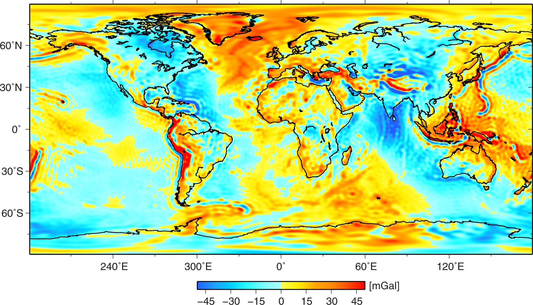
Figure 27. Monthly total mass anomaly (global mean variation removed) for the Indo-Atlantic Oceans (blue) and Pacific Ocean (red) observed by GRACE (CSR RL05), updated from Chambers and Willis [284]. The correlation between the two is −0.94, representing an exchange of mass between the Pacific and Indo-Atlantic Oceans.
Download figure:
Standard image High-resolution image
In some areas, GRACE may be able to detect transport variation for a specific current system. One such current is the ACC, which has measureable currents to the sea floor. When the geostrophic transport varies, it has to be balanced by changing pressure across the current, which should be observable by GRACE. This is important, as measuring the transport of the ACC and especially its low-frequency variability is difficult. This can only be done directly by measuring temperature and salinity along a North–South transect of the ACC, such as along the Drake Passage, then estimating geostrophic current shear. However, this is only precise if the measurements are made to the bottom, and a current reading is also made at some depth as a reference, neither of which has been done more than a handful of times due to the expense [285]. Errors by not measuring to depth and assuming a reference velocity of zero can be of the order of 25 Sv or more. Other estimates have been made using bottom pressure gauges based on some assumptions that simplify the problem (e.g. [286]). However, since these sensors drift, it is difficult to determine long-term changes in transport with any certainty. Climate models have predicted a poleward movement and strengthening of the Southern Ocean winds and the ACC in a warming world (e.g., [287]), so there is a need to measure whether the transport is increasing to confirm the models.
While there have been attempts to measure the transport of the Antarctic Circumpolar Current with GRACE, all have focused on seasonal and shorter period fluctuations, and for averages over large areas, generally the size of the Pacific sector of the ACC, and have included portions of the transport that does not pass through the Drake Passage [288–290]. Results show generally good agreement with the seasonal and higher frequency variability predicted by models, with differences of about 3 Sv RMS. Little work has been done to evaluate low-frequency variations, however, except for some evaluation of correlations between GRACE-derived transport for the ACC averaged over the Pacific sector and the Southern Annual Mode (SAM) [290]. The SAM is often used as an index of wind variability over the Southern Ocean, and has variations from a few weeks to many decades. Although correlations between GRACE-derived transport and SAM have been shown to be high [290], the results are likely biased by the high-frequency and seasonal variability. No analysis was done for the longer than annual period. However, assuming monthly errors of 3 Sv with a random autocorrelation, a change in transport of less than 0.3 Sv/year should be detectable by GRACE with 90% confidence using the current 10-year record.
Most oceanograpic studies using GRACE focus on large-scale phenomena, occurring in the open ocean. This is partly due to the fact that locally, the amplitude of OBP signals generally falls below the noise level of GRACE. Near the coast, the comparably weak OBP variations are obscured by signal leakage from nearby land hydrology, due to the limited spatial resolution of GRACE. An exception are shallow semi-enclosed shelf zones, where the water column is generally well mixed and wind stress is distributed over a relatively thin column, leading to predominantly barotropic variability. GRACE has been used to identify large OBP variations in the Gulf of Carpentaria (Australia) [291] and the Gulf of Thailand [292], with a seasonal amplitude of 20 cm and more. Interestingly, the hydrological signals over land captured by GRACE can also be used to infer OBP variations in the oceans. As explained in section 3, changes in mass loading on land will alter the gravitational pull on the ocean, so that water moving from land to ocean will not be distributed as a uniform layer in the ocean. Continental mass anomalies from GRACE have been used as input in the sea-level equation to show that meltwater from land ice will lead to an above-average sea level rise between 40°N/S [293] and that seasonal water exchange between land and ocean leads to non-uniform relative sea-level variations of ∼2 to 17 mm, with a distinct North–South gradient [294, 295]. Another oceanograpic application where GRACE has lead to advancement is modeling of ocean tides. Tidal models rely heavily on SSH observations from satellite altimetry. These observations do not always cover the high latitudes, so that empirical tidal models are relatively poorly constrained in polar areas. Various studies have used the GRACE intersatellite range-rate observations to invert local tidal mass variations and revealed tidal variations not predicted by tidal models, in particular in the Arctic [296] and Antarctic (e.g., [36, 297] regions.
6. Conclusions and perspectives
Over the past decade, GRACE has gone from being an experimental measurement needing to be verified by more trusted in situ data, to a respected tool for Earth scientists representing a fixed bound on the total change in water storage over medium to large regions. Terrestrial water storage can now be measured at large scales and in remote areas, the mass balance of the ice sheets and larger ice caps and glaciers can be monitored at an unprecedented temporal resolution, and the exchange of water masses between ocean regions can be tracked directly. Whereas with the original RL01 data, only large seasonal signals were confidently visible above the processing errors, the newest release (RL05) brings with it lower errors and a far larger selection of possible uses. Due to the improved data quality, the expertise in handling and interpreting this new data product gained since the mission launch and the increasing interaction between GRACE processors and researchers from other fields, the focus of GRACE-related research has moved from simply observing variations in water storage to explaining and interpreting these observations. Earth system modelers and GRACE processors are now engaged in an iterative cycle of mutual improvement for their products and GRACE has become a popular tool to validate and tune Earth system models, especially in hydrology (e.g., [64, 65]) and glaciology (e.g., [197, 235, 298]). GRACE data are nowadays being directly assimilated into ocean [299] and hydrology [67, 70] models and are also fed into model simulations to assess the impacts of climate change, such as the potential weakening of the Atlantic meridional overturning due to increased meltwater input from the Greenland Ice Sheet [300]. Furthermore, the mission has already lead to a successful spin-off, the Gravity Recovery and Interior Laboratory (GRAIL), which mapped the Moon's gravity field in 2012, using basically the same concept as GRACE.
With a mission length of more than 11 years and counting, the nominal 5-yr mission lifetime has long been exceeded. Both satellites still operate nominally, and with the current low solar activity (leading to less atmospheric drag), the cold gas reserves of the satellites' attitude and orbit control system are expected to last until 2018–2019. The batteries, however, are starting to feel their age. Over the years, the capacity of the battery cells has degraded and one of the two satellites has suffered two cell failures. Measures have been taken to extend the battery lifetime. Since 2011, no scientific data are collected when the sun is positioned unfavorably with respect to the satellites' orbit and the solar arrays cannot collect sufficient energy. This occurs about every 161 days, but, if a third battery cell should fail, there would be a data gap every 30–50 days. A follow-on mission has been approved and funded and is planned to be launched in 2017. This will be almost a carbon-copy of the current GRACE mission, but with evolved versions of some of the components (such as the KBR, GPS and accelerometer systems) and includes an experimental laser link between the two satellites to prove the feasibility of much more precise laser intersatellite ranging for future gravity missions.
The fact that the GRACE satellites sense mass redistribution as one measurement can either be seen as an advantage (e.g., in hydrology, where total terrestrial water storage can be measured directly), or as a limitation (e.g., when studying the cryosphere, where trends in ice mass are difficult to separate from GIA). This is inherent in the mission principle and is very unlikely to change in future GRACE-like missions. However, for other characteristics of the GRACE observations, there is room for improvement. A reduction of the North–South striping and the noise level in general, would lead to a more accurate estimation of the mass redistribution. Since this reduces the need for smoothing and post-processing, it would also allow a higher spatial resolution, and thus a better separation of individual signals (e.g., between hydrological and oceanographic signals in coastal regions). The quality of submonthly gravity solutions may also improve, although there will always be a trade-off to be made between an acceptable noise level and spatial resolution, and the temporal resolution, since a sufficiently dense groundtrack coverage is required. Several conceptual studies for a redesigned GRACE successor are being carried out, funded nationally and by space agencies such as ESA and NASA, with input from the broad international user community. Various new mission architectures are being considered, such as two pairs of satellites in different orbital planes, which would substantially increase the spatial resolution and reduce the North–South striping problem (e.g., [301–303]). Such a GRACE II mission is expected to be launched in the 2020s, which would ensure the long-term availability of time-variable gravity and allow the scientific community to continue to monitor changes in, and improve our understanding of, the Earth's water cycle and large-scale mass redistribution in its interior.
Acknowledgments
The authors would like to thank the anonymous reviewer and editor for their helpful and constructive comments, and Volker Klemann and Srinivas Bettadpur for commenting on parts of the manuscript. Shin-Chan Han, Andreas Hoechner, Rasmus Houborg, Volker Klemann, Marc Leblanc, Matthew Rodell, Holger Steffen and Sean Swenson are acknowledged for sharing their figures, and M King, R Bingham and P Moore for updating and sharing their Antarctica trend numbers. B Wouters is funded by a Marie Curie International Outgoing Fellowship within the 7th European Community Framework Program (FP7-PEOPLE-2011-IOF-301260). I. Sasgen acknowledges support from the DFG priority program SPP1158 'Antarctic Research' through grant SA 1734/4-1. J A Bonin and D P Chambers were both supported under NASA Grant NNX12AL28G from the GRACE Science Team.