


ABSTRACT
We investigate the outflows associated with two halo coronal mass ejections (CMEs) that occurred on 2006 December 13 and 14 in NOAA 10930, using the Hinode/EIS observations. Each CME was accompanied by an EIT wave and coronal dimmings. Dopplergrams in the dimming regions are obtained from the spectra of seven EIS lines. The results show that strong outflows are visible in the dimming regions during the CME eruption at different heights from the lower transition region to the corona. It is found that the velocity is positively correlated with the photospheric magnetic field, as well as the magnitude of the dimming. We estimate the mass loss based on height-dependent EUV dimmings and find it to be smaller than the CME mass derived from white-light observations. The mass difference is attributed partly to the uncertain atmospheric model, and partly to the transition region outflows, which refill the coronal dimmings.
Export citation and abstract BibTeX RIS
1. INTRODUCTION
Coronal mass ejections (CMEs) are large-scale activities on the Sun. The causes and consequences of CMEs are hot topics in both solar physics and space-weather research. Recently, the connection between CMEs and coronal dimmings attracted much attention. Coronal dimming, originally called the "dark area," was probably first mentioned by Evans (1957). The first compelling dimming observation was presented by Hansen et al. (1974). They found the abrupt depletions of the inner corona that are associated with Hα prominence eruption. Using observations from the X-ray telescope aboard Skylab (Vaiana et al. 1977), Rust & Hildner (1976) observed an expanding arch that is shown as apparent depletions in X-ray images and corresponded to a white-light transient (CME) in the outer corona. Since then the coronal dimmings have been studied by many authors.
There are two types of dimmings. One is small-scale twin dimmings, which are located at the two ends of a preflare sigmoid structure (Sterling & Hudson 1997). These dimmings are visible in soft X-rays (SXRs) as well as in EUV wavelengths (Zarro et al. 1999) and even in Hα (Jiang et al. 2003). However, these kinds of dimmings are observed rather exceptionally in soft X-rays (Kahler & Hudson 2001). The other are global-scale dimmings. Thompson et al. (2000) found that the large-scale dimmings originate from the source active region, and then expand across almost the entire solar disk, immediately following propagating "EIT waves." The nature of the "EIT waves" is still a controversial issue in solar physics. Some authors explained these waves as a fast-mode wave in the corona (e.g., Wang 2000; Wu et al. 2001), while some other authors considered that these are not waves (Delannée & Aulanier 1999; Chen et al. 2002, 2005; Attrill et al. 2007). Chen & Fang (2005) supposed that the "EIT waves" and the expanding dimmings are disk signatures of the leading loop and the cavity of CMEs, respectively. Indeed, dimmings, both with small scales and large scales, are interpreted as CME manifestations on the solar disk (Hudson et al. 1996; Thompson et al. 1998). Besides the scales of the two types of dimmings, they also differ in the brightness decrease. Typically, the small-scale twin dimmings are darker than the global-scale dimmings (Thompson et al. 2000).
Coronal dimmings are simultaneously visible in both the SXR and EUV bands (Zarro et al. 1999) and in separate EUV bandpasses with different formation temperatures (Thompson et al. 1998). The commencement timescale of the depletion is much shorter than the radiative cooling time (Hudson et al. 1996). All these features indicate that coronal dimmings result mainly from the loss of mass in the low corona (Thompson et al. 1998; Harrison & Lyons 2000; Harrison et al. 2003). Therefore, they are often used to estimate the mass of CMEs (Sterling & Hudson 1997; Harrison & Lyons 2000; Harrison et al. 2003; Zhukov & Auchère 2004). With numerical simulations, Chen et al. (2002, 2005) proposed that, during the CME process, the successive stretching of the closed magnetic field lines compresses the plasma on the outer side to generate EIT wave fronts. In the mean time, expanding dimmings are produced within the expanding magnetic loops. They also found that strong outflows are present in the dimming region, but absent in front of the EIT wave. This velocity pattern was in a good agreement with the Solar and Heliospheric Observatory/Coronal Diagnostics Spectrometer (SOHO/CDS) spectral results of Harra & Sterling (2001, 2003).
The EUV imaging spectrometer (EIS) on board the Hinode satellite provides EUV spectra with higher spectral and spatial resolutions than ever before, which contain many emission lines forming at different heights from the lower transition region to the corona. Therefore, the EIS observations allow us to investigate the outflows in the dimming regions in more detail. The Hinode/EIS has observed the source regions of a large number of CME events. Among these, two CME/flare events on 2006 December 13 and 14 in NOAA 10930, which were accompanied by EIT waves and coronal dimmings, were well observed by various telescopes. In particular, the EIS was pointing at the dimming region in the raster scan mode for the two events. Harra et al. (2007) studied the outflows in the dimming region of the 2006 December 14 event. It was found for the first time that the outflow exists in an extended dimming region away from the flare core, and that the strongest outflow appears in the loop footpoints. Imada et al. (2007) further showed that the CME-induced outflow is structured not only in the horizontal plane, but also in the vertical direction. Therefore, it is important to study the height dependence of the density depletion, in particular the density depletion in the chromosphere (Jiang et al. 2003), which was often neglected in the estimate of the mass supply for CMEs. In this paper, we study in detail the dimming regions in these two CME/flare events with EIS observations. In particular, we focus on how the CME-induced outflows are distributed in the three-dimensional volume and whether the plasma depletion in the coronal dimmings can account for the mass of the CME.
The paper is organized as follows. In Section 2, we describe the observations and the data analysis. In Section 3, we display the evolution of the outflows in the dimming regions. The spatial distribution of the outflows is presented in Section 4, followed by the mass loss and mass flow estimation in Section 5. The conclusions are given in Section 6.
2. OBSERVATIONS AND DATA ANALYSIS
2.1. Instrument and Observations
The EIS instrument (Culhane et al. 2007), which is aboard the Hinode spacecraft (Kosugi et al. 2007), provides spectra with high spectral resolution in two wave bands, 166–211 Å and 246–292 Å, which include many emission lines in the transition region and the corona. The four slit/slot positions, 1'', 2'', 40'', and 266'', allow a wide choice of the operation modes. Using 1'' or 2'' slits, the instrument can construct images by moving the mirror to raster an area of interest. With this mode, the spectra of each point in the field of view (FOV) are obtained, while the 40'' or 266'' slot observations provide monochromatic images of the Sun. In this paper, we use the high spectral resolution data obtained with the 1'' slit raster scan mode.
During the period of 2006 December 13 and 14, two halo CME/flare events occurred in the active region NOAA 10930. SOHO/Large Angle and Spectrometric Coronagraph (SOHO/LASCO) recorded the events starting at 02:54:04 UT on December 13 and 22:30:04 UT on December 14, respectively. Each CME was accompanied by an EIT wave, as revealed by SOHO/Extreme ultraviolet Imaging Telescope (SOHO/EIT). Coronal dimmings behind the EIT wave fronts can be clearly seen in Figure 1, which shows the EIT 195 Å base difference images at 03:00:01 UT on 2006 December 13 (left panel, the first event) and at 01:13:42 UT on 2006 December 15 (right panel, the second event). To obtain the base difference images for the two events, we subtract preflare images from the images at 03:00:01 UT (December 13) and 01:13:42 UT (December 15) for the two events, respectively, where the photospheric differential rotation (Howard et al. 1990) is taken into account by using the SSW routine DROT_MAP. The preflare images are taken at 02:12:01 UT (December 13) and 21:12:35 UT (December 14) for the two events, respectively. The dashed boxes in Figure 1 approximately show the EIS FOVs, which require ∼4.5 hr for the former scan and ∼2.3 hr for the latter one.

Figure 1. SOHO/EIT 195 Å base difference images at 03:00:01 UT on 2006 December 13 (left) and at 01:13:42 UT on 2006 December 15 (right) with preflare images at 02:12:01 UT (December 13) and 21:12:35 UT (December 14) subtracted. The dashed boxes represent the Hinode/EIS field of view in the two events.
Download figure:
Standard image High-resolution imageThe 2006 December 13 event was scanned twice by the EIS before and after the CME initiation, with a 1'' raster of 512 steps from west to east and 256'' in height. The first scan started at 19:07:20 UT and ended at 23:46:16 UT on 2006 December 12, which was prior to the eruption. The second scan started at 01:12:12 UT and ended at 05:41:39 UT on 2006 December 13, covering the main phase of the flare. In the following analysis, we define the first scan as the pre-eruption phase and the second as the eruption phase for clarity. For the 2006 December 14 event, we choose four scans for study. The four time periods are 19:20:12–21:34:55 UT on 2006 December 14, 01:15:19–03:30:02 UT, 04:10:12–06:24:54 UT, and 10:29:32–11:18:55 UT on 2006 December 15, respectively. According to the coronagraph observations recorded by the LASCO and the GOES X-ray light curve, the first scan was done before the CME. The next three scans were done ∼3, 6, and 12 hr after the flare peak time. For this event, we define the first scan as the pre-eruption phase, the second as the eruption phase, the third and fourth as the posteruption phases. Each scan consists of 256 steps, yielding a 256''× 256'' FOV, which is half that of the former event.
In the observations, nine spectral windows were recorded. In this paper, we use seven of them: Fe x 184.54 Å, Fe viii 185.21Å, Fe xii 195.12 Å, Fe xiii 202.04 Å, He ii 256.32 Å, Fe xiv 274.20 Å, and Fe xv 284.16 Å. These emission lines have different formation temperatures and can represent physical properties at different heights from the lower transition region (e.g., He ii 256.32 Å) to the corona (e.g., Fe xv 284.16 Å). Table 1 lists the emission lines included in this study and their formation temperatures. The formation heights and densities are also included in the table, which are deduced from the quiet-Sun atmospheric model VAL3C (Vernazza et al. 1981) and the coronal model of Withbroe (1988). These information will be used while estimating the mass loss in the dimming regions. However, Withbroe's model does not contain the layer corresponding to the formation temperature of Fe xiv and Fe xv; so the height and density information is not available for these two lines.
Table 1. Hinode/EIS Lines Used in This Study
| Ion | Line Center (Å) | log Tmax (K) | Height (km) | Ne (cm−3) |
|---|---|---|---|---|
| Fe xv | 284.16 | 6.30 | ⋅⋅⋅ | ⋅⋅⋅ |
| Fe xiv | 274.20 | 6.25 | ⋅⋅⋅ | ⋅⋅⋅ |
| Fe xiii | 202.04 | 6.20 | 13,3000 | 7.584 × 10⁷ |
| Fe xii | 195.12 | 6.11 | 33,600 | 2.616 × 10⁸ |
| Fe x | 184.54 | 6.00 | 21,000 | 3.196 × 10⁸ |
| Fe viii | 185.21 | 5.60 | 2543 | 1.205 × 10⁹ |
| He ii | 256.32 | 4.70 | 2280 | 9.993 × 10⁹ |
Download table as: ASCIITypeset image
2.2. Data Reduction and Line Fitting
We use the routine EIS_PREP in SolarSoftWare to calibrate the EIS data, which can correct the flat field, dark current, cosmic rays, and hot pixels. After this process, we obtain the absolute intensities in units of erg cm−2 s−1 sr−1 Å−1. We then fit each emission line with a Gaussian profile in order to determine the line center. While determining the center of a specific line, two instrumental effects should be taken into account. One is the slit tilt, because the EIS slit is not perfectly vertical on the two CCDs. The other is the orbital variation, which is caused by thermal effect on the instrument and follows a sinusoidal behavior. To remove the former, we subtract the Doppler shift taken early in the mission (regarded as purely due to the tilt effect) from the current one. This can be done by the SSW routine EIS_SLIT_TILT. To remove the latter, we first calculate the position for the rest line center for each raster that is taken to be the average of the southern part (relatively quiet region) of each slit. We then obtain the time variation of the rest line center relative to the theoretical position. After the above steps, we can finally construct the Dopplergrams for each time.
When dealing with the He ii 256.32 Å line, the blending effect should be taken into account as discussed by Young et al. (2007b). The He ii 256.32 Å line blends with three other lines: Si x 256.37 Å, Fe xiii 256.42 Å, and Fe xii 256.41 Å, where the first line is generally much stronger than the other two. Usually, we can use the Si x 261.04 Å line to estimate the contribution of the Si x 256.37 Å line because they have a fixed intensity ratio of 0.89. Unfortunately, in the observations used for our study, the Si x 261.04 Å line is not available. In order to minimize the blending effect, we use double Gaussian profile to fit the He ii 256.32 Å line. The fitting parameters are carefully chosen in order to avoid some unrealistic results. The maximum blending component is set to be 40% of the whole intensity profile. This value is twice the blending value suggested by Young et al. (2007b). In fact, the fitting results show that the majority of the blending components are well below this value especially for the dimming region. Moreover, considering the same emission temperature of the Si x 256.37 Å and Fe xii 195.12 Å lines, we assume that they have the same Doppler velocity. Since the other blending lines mentioned above may affect the line center of the Si x line, a slight offset within ±0.05 Å of the line center is allowed when choosing the best-fitting parameters. The results show that double Gaussian fitting can significantly reduce the values of χ2 for the He ii 256.32 Å line, especially in active regions, which suggests that the contribution of the Si x line is more significant in the active regions than in the dimming areas.
For the present He ii 256.32 Å observations, we do not find a relatively quiet region to calculate the rest line center. Therefore, the correction of orbital variation for the He ii 256.32 Å line should also be especially treated. After comparing many quiet-Sun observations of the EIS, we find that the orbital variation curve changes very little for a long period. Therefore, we use a quiet-Sun scan observation of the EIS on 2006 December 24, i.e., ∼10 days later, to calculate the standard orbital variation curve, and apply it to the He ii line observations in this study. After such a correction, we can finally obtain the absolute velocities for the He ii line.
2.3. Co-alignment of the Images
The first thing is that we need to correct the offsets in the N–S and E–W directions between EIS images at different wave bands. The EIS has short wave band (166–211 Å) and long wave band (246–292 Å) images. The heliocentric coordinates recorded in EIS data are calibrated only for the long wave band images. After comparing the images at different wave bands, we shift the short wave band images 16'' southward and 2'' westward relative to the long wave band images to correct for the spatial offset between them. These offset values are also consistent with the study by Young et al. (2007a).
The co-alignment between the small-scale images of the EIS and global-scale images of other instruments is a tricky issue. We solve the problem by carefully comparing the EIS and EIT images at 195 Å. Since the EIS images are reconstructed through raster scanning, each of them spans a period of several hours. In order to achieve the co-alignment as accurate as possible, we set the mid-time of the scanning as the time for the EIS image. Then, we choose an EIT image observed at the closest time and compare it with the EIS image. To make a more reliable co-alignment, we change the values of XCEN and YCEN in the EIS image reiteratively until the highest correlation coefficient is reached between the two images. Using this method, the uncertainty of the co-alignment is ±2''. If taking into account the time difference between the active and dimming region observations, the uncertainty should be somewhat larger than this value. This correction is based on the assumption that the coordinate information of SOHO/EIT observations is reliable. According to the report of the instrument (Delaboudinière et al. 1995) and its on-orbit performance (Defise et al. 1998), this is a good assumption.
3. OUTFLOWS IN THE DIMMING REGIONS
3.1. The 2006 December 13 Event
This event is very famous and has been well studied (e.g., Kubo et al. 2007; Zhang et al. 2007; Asai et al. 2008; Guo et al. 2008; Imada et al. 2008; Jing et al. 2008). In Figures 2(a) and (b), we show two Dopplergrams derived from the Fe xii 195.12 Å emission line for the two phases of the 2006 December 13 event. Figure 2(b) is the full FOV (512'' × 256'') Dopplergram. According to the EIT image in Figure 1, the left part of Figure 2(b) is the EIT dimming region and the right part is the flaring region. A blueshift pattern is clearly seen in the dimming region. In Figure 2(a), we present the Dopplergram at the pre-eruption phase for a subarea shown as the black dashed box in Figure 2(b). No significant blueshift is visible at this time. Note that during the pre-eruption phase, there exist some weak blue and redshifts in the later dimming region. They are probably caused by the flows in magnetic loops and have no clear relationship with the outflows after the eruption. For this event, we also check the Dopplergram of the posteruption phase (∼20 hr after the first appearance of the CME). In this observation, the pointing of the telescope had been changed; only a small part of the dimming region was observed. Therefore, we do not show the Dopplergram at the posteruption phase. However, the Dopplergram of the observed region implies that no significant outflows sustain in the dimming region ∼20 hr after the first appearance of the CME in the LASCO/C2 FOV.

Figure 2. Dopplergrams derived from the Fe xii 195.12 Å (panels (a) and (b)) and He ii 256.32 Å (panels (c) and (d)) spectra of Hinode/EIS at two different phases of the 2006 December 13 CME. Positive and negative velocities correspond to red and blueshifts, respectively. Panels (a) and (c) show the pre-eruption phase, while panels (b) and (d) show the eruption phase. The black dashed boxes in panels (b) and (d) represent the FOV in panels (a) and (c). The black dotted box in panel (b) shows the small region that we use to calculate the mean velocity for the seven lines.
Download figure:
Standard image High-resolution imageIn Figures 2(c) and (d), we show the He ii 256.32 Å Dopplergrams for this event. The He ii 256.32 Å line is formed at a relatively low temperature in the transition region, where the plasma dynamics should be quite different from that in the corona. It is seen that the velocities in He ii are much smaller than those in Fe xii. Moreover, from the He ii Dopplergram at the eruption phase, we can see large-scale patterns with blueshifts in the dimming region instead of several patches in Fe xii. Since the He ii 256.32 Å line is an optically thick line, the line profile is formed through radiative transfer in a medium with velocity gradients. In such cases, the Doppler velocity derived from the line centroid usually underestimates the real value. Therefore, we can expect that the actual Doppler velocities will be larger than the values deduced from the observed He ii spectra.
To compare the different results from the seven emission lines, we use the following steps to obtain the characteristic Doppler velocities for these lines. First, we select a region with an intensity drop larger than 20% of the original value. We make an average over all the blueshifts in that region to obtain the mean velocity for each line. Then, we further make an average over the points with Doppler velocities larger than 1.5 times the mean velocity. The final values are thus regarded as the characteristic velocities we plot in Figure 3. The characteristic velocities in the dimming region at the two phases are plotted using the black symbols. We also investigate the Doppler velocity changes along the height in a small region with remarkable blueshifts, indicated in Figure 2(b) by a black dotted box. The mean velocities over the selected region are shown in Figure 3 using the gray symbols. The figure shows that, at the eruption phase, all the seven lines have significant blueshifts, though the values depend on their formation temperatures. This result has been reported by Imada et al. (2007) for a certain place in the dimming region. Here, we find that this result is also valid for the Doppler velocities over a small region as well as the characteristic velocities in the dimming region. During the pre-eruption phase of the December 13 event, there are no significant blueshifts in the dimming region.
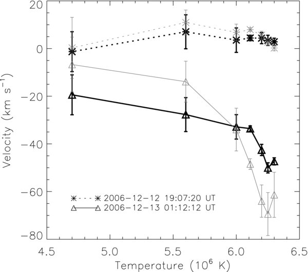
Figure 3. Doppler velocities in dependence of line formation temperatures observed by the Hinode/EIS. The two observation times represent the pre-eruption phase and the eruption phase, respectively. The black and gray symbols represent the characteristic velocities in the dimming region and the mean velocities over a small region, respectively. The error bars represent 1σ of the mean velocity.
Download figure:
Standard image High-resolution image3.2. The 2006 December 14 Event
In Figure 4, we show five Dopplergrams derived from the Fe xii 195.12 Å line for the 2006 December 14 event. Panel (a) is the full FOV (256'' × 256'') Dopplergram at the eruption phase. Compared with the EIT difference image in Figure 1, the left part of panel (a) is the dimming region and the right part occupies half of the active region. We choose a small region with the most obvious blueshifts, i.e., the black dashed box in panel (a), and plot the time series of Dopplergrams for this region in panels (b)–(e). For this event, the evolution of the Fe xii 195.12 Å velocity field is similar to that in the 2006 December 13 event.

Figure 4. Dopplergrams derived from the Fe xii 195.12 Å spectra of the Hinode/EIS for the 2006 December 14 CME. Positive and negative velocities correspond to red and blueshifts, respectively. Panel (a) is the Dopplergram of the full EIS FOV for the eruption phase: 01:15:19–03:30:02 UT. Panels (b)–(e) are time series of Dopplergrams for a subarea shown as the black dashed box in (a), which refers to (b) the pre-eruption phase: 20:22:50–21:32:49 UT on 2006 December 14, (c) the eruption phase: 02:13:44–03:23:43 UT on 2006 December 15, (d) the posteruption phase: 05:06:31–06:16:29 UT on 2006 December 15, and (e) the posteruption phase: 10:47:40–11:13:19 UT on 2006 December 15. The black dotted box in panel (a) shows the small region that we use to calculate the mean velocity for the seven lines.
Download figure:
Standard image High-resolution imageFigure 5 shows the He ii 256.32 Å Dopplergrams. At the pre-eruption phase, there are some redshift patches in the FOV; at the eruption phase, redshifts are replaced by blueshifts; at the posteruption phases, redshifts appear again in this region. Similar to the December 13 event, the He ii Dopplergram at the eruption phase shows large-scale patterns with blueshifts in the dimming region instead of only several patches shown in Fe xii. We notice the unusual blueshift pattern at the top right corner of Figure 5(b) showing the Dopplergram at the pre-eruption phase. The shape and magnitude of this blueshift pattern vary during the whole evolution. We investigate this area carefully and find that it may not correlate with the CME and outflows, since this area lies out of the dimming region, as can be seen in the right panel of Figure 1. By contrast, in the Dopplergram of Fe xii 195.12 Å observed by the EIS, this area is mainly redshifted. The EIT 195 Å observation shows that there are closed flaring loops over this area implying that outflows are unlikely to exist. Therefore, we consider that the blueshifts in this region reflect the plasma motions in the low-lying closed loops, like the circulation flows described by Marsch et al. (2008). In this study, we only focus on the blueshifts in the dimming region. Therefore, this unusual blueshift pattern is not addressed further in our analysis.

Figure 5. Dopplergrams derived from the He ii 256.32 Å spectra of Hinode/EIS for the 2006 December 14 CME. The notation of the figure is the same as Figure 4.
Download figure:
Standard image High-resolution imageIn the left panel of Figure 6, we plot the characteristic velocity variations with respect to the line formation temperatures at different phases of the event. Like the 2006 December 13 event, we also choose a small region with remarkable blueshifts (indicated by a black dotted box in Figure 4(a)) and obtain the mean velocities of this region. The result is shown in the right panel of Figure 6. Similar to the December 13 event, the velocity is the largest at the eruption phase. At the posteruption phase, the velocity decreases to the pre-eruption value. In this event, however, we do not see a strong temperature dependence of the velocity in the dimming region.
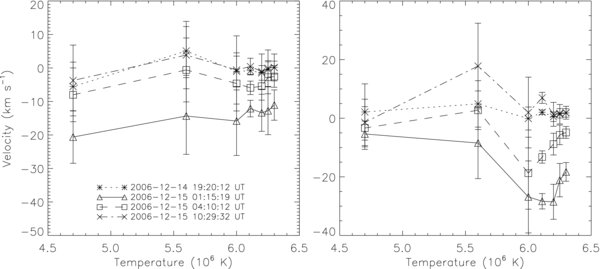
Figure 6. Doppler velocities in dependence of line formation temperatures observed by the Hinode/EIS. The four observation times represent the pre-eruption phase, the eruption phase, and the posteruption phase (the two latter times), respectively. The error bars represent 1σ of the mean velocity. The left panel shows the characteristic velocities in the dimming region. The right panel shows the mean velocities over a small region.
Download figure:
Standard image High-resolution imageUnlike the 2006 December 13 event, the data for the 2006 December 14 event are complete. Therefore, we can analyze the intensity variation of the dimming region in detail. We derive the mean intensity variation of the six emission lines in the main dimming region, i.e., the region we have used for calculating the characteristic velocity. The intensity variation is shown in the left panel of Figure 7. Intensity changes for different lines are quantitatively different, but their general trends are similar. The intensities are significantly reduced after the CME occurrence and rise gradually to the quiescent values in the later phase. We also try to use the whole dimming region to deduce the intensity variation. The result is similar only that, the magnitude of intensity drop is somewhat smaller.

Figure 7. Variation of the line intensity (left) and mass density (right) after the CME eruption on 2006 December 14–15 (normalized to the pre-eruption value).
Download figure:
Standard image High-resolution imageA reasonable assumption is that all these EUV lines are optically thin,3 which means that the line intensity scales proportional to the square of the plasma density, i.e., I ∼ ρ2. Assuming that the plasma temperature in the dimming volume did not change much, the intensity variation in the dimming region reflects the variation of the density. The estimated density variation is shown in the right panel of Figure 7. An impression is that the relative depletion is more significant in the higher layers than in the lower layers. Moreover, the density recovery times are different from line to line. For the Fe xii 195.12 Å line, at the early stage of dimming, the density decreased to ∼50% of the normal value. After ∼10 hr, the density was still lower than the initial value. However, for three other lines, Fe viii 185.21 Å, Fe xiv 274.20 Å, and Fe xv 284.16 Å, after ∼10 hr, the densities become 25%, 10%, and 30% higher than the initial value, respectively. The increased density at those layers after the eruption phase may be caused by some reasons, such as the change in the magnetic topology etc.
The gradual recovery of the EUV brightness is a typical feature of coronal dimmings (Reinard & Biesecker 2008; Attrill et al. 2008), which is correlated with the overlying corona closure and heating by the confined plasma in the closed magnetic loops (McIntosh et al. 2007). Attrill et al. (2008) proposed a model to interpret the maintained outflows during the recovery phase in which interchange reconnections are continually occurring between emerging flux in the dimming region and the opening field lines caused by CME. This is similar to the mechanism of fast solar wind. In this study, we find a general blueshift in the dimming region at the eruption phase, though according to Marsch et al. (2008) some of the blueshifts may just reflect the circulation flows along the loops and cannot get into the formation layer of the solar wind. The increased Doppler velocity at all the heights makes us believe that some flows at the height of the He ii line can sustain into the corona and contribute to the solar wind. The He ii line shows an averaged Doppler velocity of ∼9.0 km s−1 in the dimming region, which is much larger than the velocity at that layer that contributes to the fast solar wind (Tu et al. 2005). Therefore, we propose that the strong outflow is a dynamic response of the transition region to the enhanced pressure gradient as the CME eruption evacuates the plasma in the lower corona.
4. THE SPATIAL DISTRIBUTION OF THE OUTFLOWS
4.1. Outflow Velocity and Magnetic Field
In order to check the relationship between the outflow velocity and the magnetic field, we overlay the photospheric magnetograms observed by SOHO/Michelson Doppler Imager (SOHO/MDI) (Scherrer et al. 1995) on the Fe xii 195.12 Å Dopplergrams observed by Hinode/EIS. The magnetograms have been smoothed in order to highlight the main magnetic structures. The left panels of Figures 8 and 9 show the co-aligned images for the 2006 December 13 and 14 events, respectively. For each image, we select 16 small segments, each with an area of 32'' × 32''. We derive the averaged velocities and magnetic field strengths for these segments. The right panels of Figures 8 and 9 plot the magnetic field strengths against the velocities (filled circles) for the two events. It is found that the two parameters in the selected segments are positively correlated with correlation coefficients being ∼0.65 and ∼0.58 for the 2006 December 13 and 14 events, respectively. If we set a velocity cutoff of ∼10 km s−1 for the former event and ∼2 km s−1 for the latter event, the correlation coefficients rise up to ∼0.81 and ∼0.85. We also tried to divide the images into smaller segments, e.g., each has an area of 16'' × 16'', the correlation between the velocities and the magnetic field strengths is still evident, with slightly lower coefficients of ∼0.59 and ∼0.47 for the two events, respectively. Here, we also notice that the scatter seems large especially for the 2006 December 14 events. It may be caused by the asynchronous observation of the magnetic field strengths and the Doppler velocities, as well as the uncertainty of the velocities. We therefore consider that the correlation revealed in our study is statistically meaningful. However, it still needs to be checked by more observations.
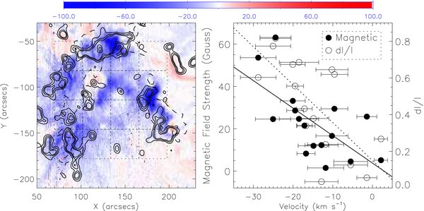
Figure 8. Left. the photospheric magnetogram (solid contours) observed by SOHO/MDI and the difference intensity map (dashed contours) observed by SOHO/EIT, overlaid on the Dopplergram (gray scale) of the Fe xii 195.12 Å line observed by Hinode/EIS at 01:12:12 UT on 2006 December 13. The solid contour levels are 30, 60, and 90 Gauss, respectively. The dashed contours represent 25% of the maximum intensity decrease in the FOV. The dotted boxes show the 16 regions used to obtain the velocities and magnetic fields. Right. relationship between the velocities and magnetic fields (filled circles) and that between the velocities and relative changes in intensity (open circles) for the 16 small gridded areas shown in the left panel. The dashed and solid lines represent the regression lines of the data. The error bars represent 1σ of the mean velocity.
Download figure:
Standard image High-resolution image
Figure 9. Left. the photospheric magnetogram (solid contours) observed by SOHO/MDI and the difference intensity map (dashed contours) observed by SOHO/EIT, overlaid on the Dopplergram (gray scale) of the Fe xii 195.12 Å line observed by the Hinode/EIS at 01:15:19 UT on 2006 December 15. The solid contour levels are 30, 60, and 90 Gauss, respectively. The dashed contours represent 25% of the maximum intensity decrease in the FOV. The dotted boxes show the 16 regions used to obtain the velocities and magnetic fields. Right. Relationship between the velocities and magnetic fields (filled circles) and that between the velocities and relative changes in intensity (open circles) for the 16 small gridded areas shown in the left panel. The dashed and solid lines represent the regression lines of the data. The error bars represent 1σ of the mean velocity.
Download figure:
Standard image High-resolution imageThe positive correlation between the velocity and the magnetic field can be understood as follows. Unlike the strongly fragmented photospheric magnetogram, the magnetic field in the corona is relatively more uniform. The magnetic flux conservation implies that a larger dimming volume in the corona topologically maps into a photospheric segment with stronger magnetic strength. Therefore, more mass flux is required from the stronger magnetic segments.
However, further inspection reveals that the discrete coronal outflow segments are almost cospatial with the photospheric magnetic segments, rather than spatially diffused. This result is not in agreement with the canopy model of quiet Sun magnetic field (Giovanelli 1980), which states that the magnetic field, which is localized in the photosphere, becomes more and more evenly distributed at any height >500–600 km above the photosphere. Correspondingly, the outflow would become more and more diffuse from the transition region to the corona, which is not seen in the EIS observations. This result may imply that either the canopy structure as in the pre-eruption phase is stretched up and the coronal magnetic field becomes less uniform or the nonlinear force-free magnetic field lines in the low corona roughly keep their nonuniform structure in the root, and do not expand toward an almost uniform distribution as expected from a potential field.
4.2. Outflow Velocity and Dimming
We also investigate the relationship between the outflow velocity and the relative change of the intensity after the CME eruption. The left panels of Figures 8 and 9 show the general shape of the main dimming region (black dashed contours) according to 25% of the maximum intensity decrease in 195 Å. It can be seen that the outflows are mainly present in the dimming regions enveloped by the dashed contours. The right panels of Figures 8 and 9 plot the relative changes of the intensity against the velocities for the same sample segments as shown in Section 4.1. It is shown that the outflow velocities are highly correlated with the relative changes of the intensity in the first event, with the correlation coefficient being ∼0.71. The correlation is much weaker for the second event, with the correlation coefficient being only ∼0.32. The low coefficient in the second event may be caused by the lower velocities that contain a high level of uncertainty. Because the relative changes of the intensity reflect the magnitude of density variation, the above results suggest that the higher the outflow velocity is the more the coronal mass is depleted.
In conclusion, faster outflows tend to be located at the regions with a stronger magnetic field, where more enhanced intensity depletion appears. Quantitatively, the outflow velocities are positively correlated with the magnetic field strengths and the magnitude of intensity depletion.
5. ESTIMATION OF THE CME MASS
Based on white-light coronagraph observations, the CME mass is estimated to be typically in the range of 2 × 10¹⁴ to 2 × 10¹⁶ g (Howard et al. 1985). Considering the mass conservation, the plasma accumulation in the leading loop is balanced by the density depletion in the dimming region. Thus, coronal dimmings, either in the EUV or X-ray, have been applied to estimate the mass of CMEs. However, it was often shown that the coronal mass depletion is smaller than the CME mass estimated from white-light emissions. For example, Harrison & Lyons (2000) found that the mass loss in the dimming region can account for only ∼70% of the total mass of the CME. In this section, we try to clarify the relationship among the CME mass, plasma depletion, and plasma filling from the lower transition region to the corona. Note that the CME mass, estimated through the SOHO/LASCO coronagraph using the CALC_CME_MASS routine in SSW, is ∼7 × 10¹⁵ and ∼3.6 × 10¹⁵ g for the December 13 and 14 events, respectively.
5.1. Mass Loss in the Dimming Region
Using the several EUV emission lines with different formation temperatures observed by the EIS, we can estimate the net mass loss in the dimming region. In this study, we choose four EIS emission lines: Fe viii 185.21 Å, Fe x 184.54 Å, Fe xii 195.12 Å, and Fe xiii 202.04 Å. The He ii 256.32 Å line is not used here, since its property of being optically thick makes it difficult to deduce the density changes from the line intensities. Because the formation temperatures of the Fe xiv 274.20 Å and Fe xv 284.16 Å lines are not included in Withbroe's model, we also do not use these two lines while estimating the mass loss. Since the upper corona is much more tenuous than the lower transition region, this has no significant influence on the final result. However, considering the strongly inhomogeneous density and temperature in the corona, we expect a small change in the estimation of the total mass loss if including these two lines. The total mass loss can be expressed as

where i represents the sequence of the four EUV lines, S(h) is the area of the EIS dimming region at different heights in the corona (with an intensity drop larger than 5% at the eruption phase compared with the pre-eruption phase); Δρ(h) is the decrement of the density at different heights in the corona. h1 is set to the formation height of the cool line Fe viii 185.21 Å, whereas h2 is set to that of the hot line Fe xiii 202.04 Å. Taking the VAL3C model (Vernazza et al. 1981) as the reference atmosphere for the transition region line (Fe viii 185.21 Å) and the coronal model of Withbroe (1988) for the coronal lines (Fe x 184.54 Å, Fe xii 195.12 Å, and Fe xiii 202.04 Å), we can determine the formation heights, h, of these emission lines. The number density of the coronal plasma (in units of cm−3) at the height h is given by the Baumbach–Allen formula (Cox 2000):
where R = R☉ + h. The formation heights and the corresponding densities of the four EUV lines in the pre-eruption phase are shown in Table 1. With the assumption that the temperature distribution keeps constant, the EUV intensity in each line, I, is proportional to the density square, i.e., I ∼ ρ2. Thus, the density variation is related to the EUV intensity variation by  , by which we can deduce the value of Δρ at different heights. The results are shown in the left panel of Figure 10. We also show the dimming area varying with the height in the right panel of Figure 10. The dimming area of the He ii 256.32 Å line is also shown in the figure using the gray symbols. In these two events, we find that the dimming area becomes larger with increasing height. If we regard the dimming region as the source of the solar wind, then the scenario in our study is very similar to that of the funnel model of the solar wind presented by Tu et al. (2005). Putting these values into Equation (1), we obtain that the mass loss is ∼4.5 × 10¹⁴ g and ∼3.4 × 10¹⁴ g for the two events, respectively. We need to discuss the possible effect of the differential emission measure (DEM) on the results. As is known, the coronal lines are formed at very thin layers with certain temperatures. While the EUV continuum is formed at a much broader region with multiple temperatures, the effect of the DEM on the coronal lines is much smaller than that on the EUV continuum and has only a slight influence on the density estimation for each line. In particular, we use the height integration to estimate the total mass loss. The effect of the DEM on the total mass loss should be quite small and insignificant. Note also that the dimming region outside the EIS FOV has little influence on the results judging from its area and magnitude.

Figure 10. Variation of Δρ (left) and dimming area (right) in dependence of height in the 2006 December 13 and 14 events.
Download figure:
Standard image High-resolution imageIt is noticed that the mass loss estimated from the EUV lines is ∼10 times smaller than the CME mass estimated from the LASCO observations. Two possible reasons may account for such a discrepancy. First, the reference atmospheric models that we adopted represent the quiet Sun, so they may not be appropriate for the atmosphere above plage regions. Above the plage regions, the density should be much higher than that described by the reference models. In order to test our supposition, we use a line pair, Fe xii 186.88 Å/Fe xii 195.12 Å, to diagnose the density of the corona (Young et al. 2007b, 2009). The EIS raster observation, we use for the density diagnostics, was started at 15:11:31 UT on 2006 December 14, which was ∼7 hr before the 2006 December 14 CME. The derived density is ∼2.3 × 10⁻¹⁵ g cm−3. However, the density that we used to calculate the mass loss is only ∼4.4 × 10⁻¹⁶ g cm−3. This means that at the formation height of the Fe xii 195.12/186.88 Å lines, the actual density can be ∼5 times the quiescent value. If we correct the results using this factor, then the mass loss for the two events will be ∼2.4 × 10¹⁵ g and ∼1.8 × 10¹⁵ g, respectively (see Table 2). Second, as indicated by the strong blueshift of the cool line He ii 256.32 Å, outflows from the lower transition region refill the coronal dimmings, which makes the coronal dimming less significant. The transition region outflow can be understood as follows: as the coronal magnetic structure is expelled outward, the plasma mass, hence gas pressure, is evacuated, which results in an extra pressure gradient in the lower corona. The transition region plasma is thus driven to move up. Such an outflow would lead to dimmings in the transition region and even in the upper chromosphere, which were discovered in Hα by Jiang et al. (2003). Therefore, the total dimmings, from the upper chromosphere to the corona, should all be taken into account in estimating the mass loss during CMEs.
Table 2. Estimate of CME Mass
| Events | Mass Loss (g) | Mass Flow (g) | LASCO Mass (g) |
|---|---|---|---|
| 2006 Dec 13 | 2.4 × 10¹⁵ | ⋅⋅⋅ | 7.0 × 10¹⁵ |
| 2006 Dec 14 | 1.8 × 10¹⁵ | a2.2 × 1016/3.3 × 1016 | 3.6 × 10¹⁵ |
Note. aThe two values correspond to different integration times (see Section 5.2).
Download table as: ASCIITypeset image
5.2. Mass Flow in the Lower Transition Region
As discussed above, the outflow in the lower transition region shown by the He ii 256.32 Å line is a natural result of the CME process. Considering mass conservation, the depletion of mass in the transition region can induce also an outflow in the upper chromosphere. The outflow refills the lower corona and compensates for the coronal mass depletion. This is one of the reasons that the dimming regions recover to the original corona after tens of hours.
In order to estimate the mass flow during the CME eruption, we choose the He ii 256.32 Å line that has the lowest formation temperature in the EIS spectrum. The mass flow is calculated by the following equation:
where ρ is the mass density at the formation height of the line, v(t) is the time-dependent Doppler velocity, and S is the area with He ii line blueshift. The density, ρ, is taken from the VAL3C model (Vernazza et al. 1981) according to the formation temperature of the emission line. When determining the Doppler velocity, v(t), we make an average over all the blueshifts in the dimming region (with an intensity drop larger than 5% at the eruption phase compared with the pre-eruption phase). The area that we use to calculate the average velocity, S, is fixed for the eruption phase and two posteruption phases.
Owing to the scanning mode of the EIS, the temporal resolution is low. We can deduce the velocities at only 2–3 times during the whole evolution of the outflows. Therefore, we fit these points to get an approximate evolution curve of the velocity.
For the 2006 December 13 event, only one scanning observation can be used to deduce the average velocity in the dimming region after the CME eruption. Owing to this fact, we do not estimate the mass flow for this event. For the 2006 December 14 event, three scanning observations are available. In Figure 11, we show the variation of the mass flow with time. The start time is set to be the beginning of the flare impulsive phase, which is ∼21:07:00 UT on 2006 December 14. We adopt both linear and exponential fits for this event. For the exponential fit, the mass flow evolves as  , where t0 is the characteristic timescale of the mass flow variation. Here, we set t0 to be the time when the mass flow decreases to half the maximum value in the linear fit. If we assume that the transition region outflow starts at the beginning of the flare impulsive phase, then it has lasted for more than 5 hr before the first EIS scanning observation. According to the exponential fit, the outflow supplies ∼2.2 × 10¹⁶ g mass during this period. In Section 5.1, we estimate the net mass loss in the corona to be ∼1.8 × 10¹⁵ g for the 2006 December 14 event. Combining these two values, the total ejected mass is roughly ∼2.4 × 10¹⁶ g. This value is much larger than the CME mass estimated from LASCO observations. This is not surprising, since this event is a halo CME, whose mass would be strongly underestimated due to the weak Thompson scattering. Also, since the mass flow has an acceleration process at the beginning and not all the mass flow can get into the corona, the difference between the mass flow and the CME mass is conceivable. We estimate the life time of the coronal dimming by fitting the time variation of the mass flow shown in Figure 11. With an exponential fitting, we find that the mass flow can last for ∼17 hr after the impulsive phase of the associated flare, during which the He ii 256.32 Å outflow refills ∼3.3 × 10¹⁶ g mass to the corona. This value can be regarded as an upper limit of the mass that the outflow in the lower transition region can supply. In Table 2, we summarize the results of CME mass estimation.

Figure 11. Temporal variation of mass flow after the CME eruption on 2006 December 14–15, using He ii 256.32 Å observation. The start time is set to be the beginning of the flare impulsive phase. The dotted and dashed lines show the linear and exponential fitting of the mass flow evolution, respectively.
Download figure:
Standard image High-resolution image
6. CONCLUSIONS
We investigate the CME-induced outflows in the dimming regions that occurred on 2006 December 13 and 14 in NOAA 10930, using the Hinode/EIS observations. We obtain the spatial distribution of the outflows, the relationship between the velocity and the magnetic field strength, and the relationship between the velocity and the relative change of the intensities. Moreover, the mass loss in the dimming volume and the lower transition region outflow are estimated. Our main conclusions are as follows.
- 1.During the CME eruption, strong outflows appear in the dimming regions at different heights of the solar atmosphere, and the outflow velocity decreases gradually with time.
- 2.The outflows are concentrated at the patches with a strong photospheric magnetic field. The larger the magnetic field strength, the faster the outflow velocity.
- 3.The outflow velocities are positively correlated with the relative changes of the intensity during the CME eruption, which suggests that more the coronal mass is depleted, higher is the outflow velocity.
- 4.The net mass loss in the dimming region estimated from the several EUV lines is ∼1015 g, which is smaller than that estimated from the LASCO observations. The discrepancy would significantly be reduced if we assume an atmospheric model that is several times denser than the quiet-Sun model and if the integration of the dimming volume extends down to the chromosphere.
- 5.There is a significant mass supply from the lower transition region to refill the coronal dimmings, which finally helps the coronal dimmings to recover to normal. We propose that this is mainly due to the dynamic response of the transition region to the enhanced pressure gradient as the CME eruption evacuates the plasma in the low corona.
We are very grateful to the referee for valuable comments that helped improve the paper. We thank the Hinode/EIS, SOHO/EIT, SOHO/MDI, and SOHO/LASCO consortiums for providing the data. SOHO is a project of international cooperation between ESA and NASA. Hinode is a Japanese mission developed and launched by ISAS/JAXA, with NAOJ as domestic partner and NASA and STFC (UK) as international partners. It is operated by these agencies in co-operation with ESA and NSC (Norway). This work was supported by National Natural Science Foundation of China (NSFC) under grants 10673004 and 10828306, and by NKBRSF under grant 2006CB806302.
Footnotes
- 3
Note that this assumption may be inappropriate for the He ii 256.32 Å line that is optically thick. Therefore, we do not show the intensity and density variation of this line in Figure 7.