


ABSTRACT
We present the results of a Herschel-PACS study of a sample of 97 low-ionization nuclear emission-line regions (LINERs) at redshift z ∼ 0.3 selected from the zCOSMOS survey. Of these sources, 34 are detected in at least one PACS band, enabling reliable estimates of the far-infrared LFIR luminosities, and a comparison to the FIR luminosities of local LINERs. Many of our PACS-detected LINERs are also UV sources detected by GALEX. Assuming that the FIR is produced in young dusty star-forming regions, the typical star formation rates (SFRs) for the host galaxies in our sample are ∼10 M☉ yr−1, 1–2 orders of magnitude larger than in many local LINERs. Given stellar masses inferred from optical/NIR photometry of the (unobscured) evolved stellar populations, we find that the entire sample lies close to the star-forming "main sequence" for galaxies at redshift 0.3. For young star-forming regions, the Hα- and UV-based estimates of the SFRs are much smaller than the FIR-based estimates, by factors ∼30, even assuming that all of the Hα emission is produced by O-star ionization rather than by the active galactic nuclei (AGNs). These discrepancies may be due to large (and uncertain) extinctions toward the young stellar systems. Alternatively, the Hα and UV emissions could be tracing residual star formation in an older, less obscured population with decaying star formation. We also compare LSF and L(AGN) in local LINERs and in our sample. Finally, we comment on the problematic use of several line diagnostic diagrams in cases with an estimated obscuration similar to that in the sample under study.
Export citation and abstract BibTeX RIS
1. INTRODUCTION
Galaxies containing low-ionization nuclear emission-line regions (LINERs) are characterized by optical emission lines including [O iii] λ5007, [O ii] λ3727, [N ii] λ6584, [S ii] λ6717, 6731, and hydrogen Balmer lines. All these lines are prominent in active galactic nuclei (AGNs) but in LINERs the relative intensities indicate a low ionization state (e.g., Heckman 1980; Ho 2008). The lower level of ionization compared with Seyfert 2 galaxies, for example (hereafter "high ionization type-II AGNs"), manifests itself in several ways, such as by the [O iii] λ5007/Hβ line ratio that is 3–5 times smaller in LINERs. In the local universe, LINERs are found in about 1/3 of all galaxies brighter than BT = 15.5 mag. This is larger than the number of high ionization type-II AGNs by a factor of 10 or more (e.g., Ho et al. 1997). Local high ionization AGNs and LINERs are present in galaxies with similar bulge luminosities and sizes, neutral hydrogen gas (H i) contents, optical colors, and stellar masses (Ho 2008).
Explanations for the origin of LINERs include shock excitation (e.g., Nagar et al. 2005; Dopita et al. 1997) and photoionization by evolved (pAGB) stellar populations (e.g., Annibali et al. 2010). However, photoionization by a low-luminosity AGN is likely responsible for many if not most LINERs, especially those with relatively bright (EW > 3 Å) Hα lines (Ferland & Netzer 1983; Barth et al. 1998; Maoz et al. 2005; Ho 1999; Gonzalez-Martin et al. 2006). Indeed, some LINERs show UV continuum variations (Maoz et al. 2005) and spectral energy distributions (SEDs) typical of accretion onto massive black holes, and contain nuclear hard X-ray sources more luminous than expected for a normal population of X-ray binaries. They also contain compact nuclear radio sources similar to those seen in AGNs (e.g., Nagar et al. 2000; Falcke et al. 2000). Various studies (Kewley et al. 2006; Ho 2008; Kauffmann & Heckman 2009; Netzer 2009) show that nuclear excited LINERs and high ionization type-II AGNs form a continuous sequence in normalized accretion rate, L/LEdd, with LINERs at the low end of the sequence.
As for all AGNs, LINERs can be classified into type-I (broad emission lines) and type-II (only narrow lines) sources. The broad lines, when observed, are seen almost exclusively in Hα but hardly ever in Hβ. This is most likely due the weakness of the broad wings that are difficult to observe against the strong stellar continua. In many cases, the classification is ambiguous and the relative number of type-I and type-II LINERs is uncertain even at very low redshift (see Ho 2008).
There have been several recent publications concerning the infrared (IR) properties of LINERs. Sturm et al. (2006) studied 33 LINERs with Spitzer. More than half are from the revised Bright galaxy survey (Veilleux et al. 1995) and are hence very bright in the IR with 12 sources showing ULIRG or LIRG luminosities. Their sample includes two different populations of LINERs: IR faint, with emissions arising mostly in compact nuclear regions, and IR luminous, which often show spatially extended, non-AGN emissions. The two populations are distinguished by their mid-IR (MIR) continuum SEDs, the luminosities of polycyclic aromatic hydrocarbon features, and mid-IR fine-structure emission lines. IR-luminous LINERs have MIR SEDs typical of starburst galaxies while the MIR SEDs of IR-faint LINERs are considerably bluer. Strong, highly excited [O iv] emissions are detected in both populations, indicative of AGN photoionization. According to Sturm et al. (2006), the two LINER groups occupy different regions of the MIR emission-line excitation diagrams.
Dudik et al. (2009) considered a sample of 67 LINERs observed with Spitzer, including many of the Sturm et al. (2006) objects. They found AGN signatures, such as the [Ne v]14.32, 24.31 μm line, in 26 sources and concluded that many of the AGN sources in LINERs are heavily obscured, even in the MIR. The fraction of AGNs is as high as 74% if all AGN diagnostics (including X-ray) are included. The mean redshift of these sources is small, with only some objects at z > 0.05. The median IR luminosity (LIR) in this sample is about 1043.5 erg s−1 with eight sources with LIR > 1044.5 erg s−1. Some very luminous IR galaxies (ULIRGs with LIR > 1045.6 erg s−1) also display LINER-like optical spectra. However, in these sources, the optical emission lines may be produced in shocked gas, rather than by AGN photoionization.
In this paper, we present new FIR Herschel photometry for a sample of z ∼ 0.3 optically selected LINERs. A visual inspection of Hubble Space Telescope (HST) images of our sample galaxies shows that most of them are late-type galaxies. Classifying such sources by their emission-line spectrum, in particular estimating the contribution to their Balmer lines from SF regions, is not a trivial issue since some emission from H ii regions is present in almost all galaxies. This is particularly problematic at intermediate and high redshifts, where even a narrow slit can cover a large fraction of the host galaxy. Large aperture UV observations of LINER galaxies, such as those commonly provided by GALEX, can also confuse a nuclear UV continuum source (in the case of type-I LINERs) with more extended UV emission from SF regions in the host galaxy. Also, a redshift of 0.3 is large enough to prevent the detection of a weak nuclear X-ray source typical of nearby LINERs. The primary goal of our paper is to use the FIR measurements to infer the global star formation rates (SFRs) of the LINER host galaxies.
2. OBSERVATIONS
2.1. Optical Observations
The zCOSMOS-bright survey includes about 20,000 galaxies with 0.1 < z < 1.2 and iAB < 22.5 mag within the 1.7 deg2 COSMOS ACS field6 (centered on 10h00m28 6, +02d12m21s). Objects in this field were observed with the VIMOS spectrograph on the Very Large Telescope (Lilly et al. 2007) and those discussed here are from the first 10,000 COSMOS objects. Bongiorno et al. (2010) selected 213 type-II AGNs from the sample for which they measured redshifts, line fluxes, and equivalent widths after removing the stellar continuum through their automated pipeline (platefit_vimos). They also derived aperture correction factors in the iAB band to take into account the small slit size (1''). The objects span the redshift range 0.15 < z < 0.92 and the luminosity range 105.5 L☉ < L([O iii] λ5007) < 109.1 L☉, where L([O iii] λ5007) is the extinction corrected [O iii] λ5007 luminosity. Bongiorno et al. (2010) combined their sample with type-II AGNs drawn from the Sloan Digital Sky Survey (SDSS) data release 7 (DR7). The additional sample included 291 objects with 0.3 < z < 0.83 and 107.3 L☉ < L([O iii] λ5007) < 1010.1 L☉. Using the combined sample, they found that type-II AGN evolution is well described by a luminosity-dependent density evolution model.
Among the 213 zCOSMOS-bright type-II AGNs, 97 objects are classified as LINERs using standard BPT (Baldwin Phillips & Terlevich 1981) classification based on [N ii]/Hα and/or [S ii]/Hα versus [O iii]/Hβ. All line fluxes were corrected for reddening based on the observed Hα/Hβ line ratio and the galactic extinction law. The requirement to measure Hα and the adjacent [N ii] λ6584 emission line limits the redshift of this group to z ⩽ 0.445. The classification is based only on sources with S/N > 3 for [O iii] λ5007 and S/N > 2.5 for the other emission lines.
We took extra care to avoid composite sources by using two boundaries defined by Kewley et al. (2001) and Kauffmann et al. (2003), see Figure 1. The theoretical curve estimated by Kewley et al. (2001) has been lowered on both the [O iii]/Hβ and [N ii]/Hα axes through SDSS observations by Kauffmann et al. (2003). Objects populating the transition region are supposed to be transient/composite star-forming-AGN sources. We classify objects as LINERs only if both line ratios are higher than those calculated by Kewley et al. (2001) and lie beyond the empirical Seyfert-LINER division (Cid Fernandes et al. 2010). Five sources (804573, 825006, 825904, 832902, 842079) have been classified as LINERs according to both [N ii] λ6584 and [S ii] λ6717, 6731. Two of the sources (819596 and 827400) do not have reliable [N ii] λ6584 measurements and were classified according to [S ii] λ6717, 6731/Hα. The classifications of the other 17 objects are based only on [N ii] λ6584, because [S ii] λ6717, 6731 are unreliable. 5 of the latter 17 sources were found to have less reliable line ratios after the publication of Bongiorno et al. (2010). We include these sources and flag them in all tables but not in diagrams because they do not show any peculiar behavior. The signal-to-noise ratio (S/N) of all observations is too low to search for weak broad Hα lines, and we consider all our objects to be type-II LINERs.
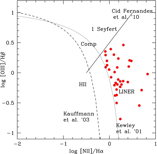
Figure 1. BPT diagram of the LINERs in our sample. The dotted line marks the separation between AGN and starburst galaxies (Kewley et al. 2001). The dashed line defines the region with composite objects (Kauffmann et al. 2003) and the solid line divides LINERs from Seyfert 2 galaxies (Cid Fernandes et al. 2010).
Download figure:
Standard image High-resolution image2.2. Herschel Observations
The above sample of zCOSMOS LINERs was observed by Herschel-PACS as part of the PACS Evolutionary Probe survey (PEP; Lutz et al. 2011). PEP is a guaranteed-time key program to survey the extragalactic sky with the aim of studying the rest-frame far-IR emission of galaxies up to redshift ∼3. PEP blank fields include COSMOS, Lockman Hole, E-CDFS, Groth Strip, GOODS-S and GOODS-N.7 Data processing, map computing, and source extraction are described in Berta et al. (2010).
Out of the 97 LINERs in our sample, 34 have σ > 3 detections in the 100 μm and/or the 160 μm PACS bands (the 3σ limits are 5 mJy and 11 mJy, respectively; see, e.g., PEP COSMOS v. 2.0, 2010 October). The archive reveals five more SDSS LINERs in the COSMOS field that were detected by Herschel. These sources have composite H ii/LINER spectra, and hence we do not include them in the sample of "pure" LINERs considered here. The positions of the PACS-detected LINERs in the BPT diagram are shown in Figure 1.
Of the 34 Herschel LINERs, 18 are detected at both 100 μm and 160 μm, 12 only at 100 μm and 4 only at 160 μm. The redshift range of these sources is 0.255–0.445. More information is provided in Table 1. The remaining 63 zCOSMOS LINERs with σ < 3 are considered non-detections. Among these 63 sources, 40 have optical line S/N > 3 and we stacked them in two subgroups according to the estimated stellar masses of the host galaxies (M*≶109.5 M☉, see Section 3, we chose this threshold in order to obtain subgroups with a similar number of objects) and found LIR=1.68 ± 0.34 × 10¹⁰ L☉ for M* > 109.5 M☉ and LIR < 0.66 × 10¹⁰ L☉ for M* < 109.5 M☉, considering z ∼ 0.3. This allows us to obtain mean M* and SFR, under different assumptions for those sub-samples, as described below.
Table 1. Sample
| ID | z | R.A. | Decl. | Herschel | Herschel | Spitzer | FUV | eFUV | NUV | eNUV | β | Morphology |
|---|---|---|---|---|---|---|---|---|---|---|---|---|
| (deg) | (deg) | PACS 100 μm | PACS 160 μm | IRAC, MIPS | (μJy) | (μJy) | (μJy) | (μJy) | a | |||
| 804277 | 0.361 | 150.41975 | 1.7757300 | X | X | X | 1.45 | 0.10 | 3.83 | 0.12 | −0.41 | 1 |
| 805283 | 0.266 | 150.19297 | 1.7524000 | X | X | X | 3.12 | 0.11 | 7.34 | 0.15 | −0.12 | 2 |
| 810944b | 0.347 | 150.34825 | 1.9489800 | X | X | X | 0.24 | 0.08 | 1.12 | 0.21 | −1.79 | 2 |
| 812596 | 0.342 | 149.98805 | 1.8229900 | X | X | ... | 2.41 | 0.11 | 5.62 | 0.15 | −0.10 | 2 |
| 816998b | 0.425 | 150.41833 | 2.0851500 | X | X | X | 0.77 | 0.14 | 1.78 | 0.14 | −0.07 | 2 |
| 818160 | 0.347 | 150.18249 | 2.0393300 | X | X | ... | 1.22 | 0.32 | 1.75 | 0.42 | 1.10 | 2 |
| 818453 | 0.360 | 150.12748 | 2.1122300 | X | X | ... | ... | ... | ... | ... | ... | 2 |
| 819347 | 0.356 | 149.92088 | 2.0312300 | X | X | X | ... | ... | 2.93 | 0.51 | ... | 2 |
| 820454 | 0.354 | 149.63649 | 2.0201200 | X | X | ... | 1.18 | 0.12 | 3.90 | 0.20 | −0.96 | 2 |
| 825006 | 0.345 | 150.06764 | 2.2429900 | X | X | X | 0.89 | 0.10 | 3.69 | 0.13 | −1.52 | 2 |
| 825904 | 0.344 | 149.89498 | 2.2084100 | X | X | X | 2.74 | 0.36 | 7.04 | 0.59 | −0.34 | 3 |
| 827762 | 0.282 | 149.50944 | 2.2318800 | X | X | X | 4.47 | 1.55 | 6.12 | 1.46 | 1.22 | 2 |
| 827818 | 0.305 | 149.49485 | 2.2806500 | X | X | X | 0.52 | 0.09 | 2.14 | 0.11 | −1.51 | 3 |
| 833627 | 0.373 | 149.74729 | 2.3457300 | X | X | ... | 1.17 | 0.14 | 6.41 | 0.15 | −2.21 | 2 |
| 839646 | 0.346 | 149.97569 | 2.4614300 | X | X | X | ... | ... | 2.43 | 0.06 | ... | 2 |
| 845649 | 0.305 | 150.16024 | 2.6993000 | X | X | X | 1.46 | 0.10 | 3.39 | 0.16 | −0.08 | 2 |
| 845945 | 0.350 | 150.10801 | 2.6955500 | X | X | X | 1.89 | 0.15 | 3.15 | 0.15 | 0.73 | 1 |
| 848329 | 0.353 | 149.58770 | 2.7614100 | X | X | ... | 1.56 | 0.13 | 2.58 | 0.15 | 0.75 | 2 |
| 818456b | 0.382 | 150.12730 | 2.0818700 | ... | X | ... | ... | ... | ... | ... | ... | 2 |
| 827400b | 0.379 | 149.59808 | 2.1583900 | ... | X | ... | 0.40 | 0.09 | 0.79 | 0.09 | 0.31 | 2 |
| 834427 | 0.445 | 149.59079 | 2.4282400 | ... | X | ... | 1.07 | 0.10 | 2.03 | 0.09 | ... | 2 |
| 838271 | 0.376 | 150.22023 | 2.5245400 | ... | X | X | ... | ... | 1.32 | 0.36 | ... | 1 |
| 804573 | 0.309 | 150.34526 | 1.6993800 | X | ... | ... | 0.84 | 0.20 | ... | ... | ... | 1 |
| 808018 | 0.284 | 149.57618 | 1.6434400 | X | ... | ... | 0.77 | 0.22 | 1.19 | 0.53 | 0.90 | 2 |
| 812330b | 0.439 | 150.04893 | 1.9487800 | X | ... | ... | ... | ... | ... | ... | ... | 2 |
| 818225 | 0.310 | 150.17228 | 2.0060500 | X | ... | ... | 0.64 | 0.13 | 1.94 | 0.26 | −0.77 | 2 |
| 819241 | 0.356 | 149.94342 | 2.0962300 | X | ... | ... | ... | ... | ... | ... | ... | 3 |
| 819596b | 0.417 | 149.86483 | 2.0032800 | X | ... | ... | 0.82 | 0.26 | ... | ... | ... | 2 |
| 823616 | 0.255 | 150.36183 | 2.2647600 | X | ... | ... | 4.40 | 0.12 | 7.83 | 0.16 | 0.58 | 2 |
| 830317 | 0.374 | 150.38441 | 2.3912700 | X | ... | ... | 0.43 | 0.14 | 2.01 | 0.22 | −1.83 | 2 |
| 832130 | 0.371 | 150.03523 | 2.4151200 | X | ... | ... | ... | ... | 0.72 | 0.23 | ... | 1 |
| 832902 | 0.333 | 149.88401 | 2.4583800 | X | ... | ... | 4.25 | 1.74 | 14.69 | 2.67 | −1.08 | 2 |
| 833279b | 0.426 | 149.81184 | 2.4412200 | X | ... | ... | ... | ... | ... | ... | ... | 2 |
| 842079 | 0.419 | 149.47718 | 2.5823700 | X | ... | ... | 0.61 | 0.07 | 0.89 | 0.09 | ... | 1 |
Notes. aIPAC Infrared Science Archive (IRSA)—Cassata Morphology Catalog v1.1: (1) elliptical; (2) spiral; (3) irregular. bOptical lines S/N < 3.
Download table as: ASCIITypeset image
2.3. Spitzer Observations
We found 13 of the 34 PACS-detected sources to have mid-IR photometric observations by Spitzer-IRAC (3.6, 4.5, 5.6, 8.0 μm) and Spitzer-MIPS (24, 70, 160 μm). We obtained Spitzer photometry for these sources from Kartaltepe et al. (2010), assuming the separation between the optical and MIR positions is less than 4'' (the MIPS angular resolution at 70 μm is about 8'').
All the sources, excepting 818456 and 812330, have been detected at 24 μm and are included in the S-COSMOS MIPS 24 Photometry Catalog, 2008 October.
2.4. GALEX UV Observations
Among the sample of 34 PACS-detected LINERs, 23 have both GALEX near-UV (NUV, peak at 2271 Å) and far-UV (FUV, peak at 1528 Å) detections within 2'' from the center of the optical images. The angular resolution in the FUV band is 2 5–35 and in the NUV band 35–5'' (Bianchi & GALEX Team 1999) and we consider those as real UV detections. Two objects have only FUV detections and four only NUV detections. Thus, 85% the PACS-detected LINERs have at least one UV detection. Out of the 63 LINERs that were not detected by PACS, 39 were detected by GALEX in both bands, 7 only in the FUV band and 10 only in the NUV band, i.e., 90% of the PACS non-detected sources have at least one GALEX detection. Data for the UV sources were retrieved from the GALEX archive8 and are given in Table 1. We find that LINERs detected by PACS are marginally brighter in the UV, see Figure 2.
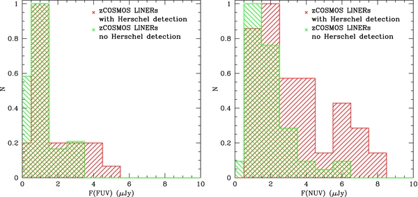
Figure 2. FUV (left panel) and NUV (right panel) flux distribution for LINERs that have been detected in the FIR by Herschel-PACS or not. FIR-detected sources have a slightly higher UV flux.
Download figure:
Standard image High-resolution imageWe used the data from the two GALEX bands to calculate the UV spectral slope, β, assuming Fλ∝λβ (see Table 1). This index is considered a good indicator of dust extinction in LIRGs and other SF galaxies at high redshift (e.g., Meurer et al. 1999; Seibert et al. 2005). The GALEX bands, especially the NUV band, are very broad, which affects our estimates of the spectral slopes. For each β, we can then estimate the rest-wavelength 1528 Å flux, which we then combine with the derived extinction to estimate the UV-based SFR (Section 3).
Meurer et al. (1999), Bouwens et al. (2009), Gallerani et al. (2010), and several others provided empirical relationships between the absorption in the UV (e.g., A(1600 Å)) and β. We derived a similar expression for the objects in our sample based on a Calzetti-type extinction law of the form Aλ∝λ−0.7 (Calzetti et al. 1994). This gives,

The extinction corrected UV fluxes and luminosities are discussed in Section 3.3.
3. STAR FORMATION RATES AND STELLAR MASSES IN LINER HOST GALAXIES
3.1. Star Formation Rate Calibrations
The primary SFR indicators we are considering in this paper are the far-IR luminosity LIR = L(8–1000 μm) as measured by Herschel-PACS and additional information provided by the extinction corrected Hα luminosity L(Hα), the extinction corrected UV monochromatic luminosity Lν(UV) measured at 1528 Å rest wavelength, and SED fitting to the extinction corrected multi-band photometry of our sources.
In using LIR as an SFR indicator, the operational assumption is that a significant (dominant) fraction of the total bolometric stellar luminosity (L*) of the star-forming population is absorbed and reradiated as thermal infrared dust emission. For an unobscured population, L* is simply the total luminosity of the directly observable stellar population. In converting an extinction corrected L(Hα) to an SFR, it is assumed that all of the ionizing Lyman continuum photons emitted by short-lived massive O-type stars are absorbed, photoelectrically, in the surrounding H ii regions with no competition from internal dust. Lν(UV) is a direct measure of starlight produced by mixtures of O-, B-, and A-type stars.
For the SFR calibrations, we have used our synthesis code STARS (Sternberg 1998; Sternberg et al. 2003) to compute L*, L(Hα) and Lν(UV) as functions of the "present-day" instantaneous SFRs (M☉ yr−1), for a wide range of galaxy ages and star formation histories. As is standard, we assume that the SFRs vary exponentially as

where t is the age of the stellar population, τ is the "decay timescale" of the star formation activity, and R0 is the initial SFR at t = 0. In the calculations, we assume Kroupa/Chabrier initial mass functions (IMFs) for the stellar populations (Kroupa 2001). We consider ages t from 1 to 103 Myr, and decay timescales τ equal to 10, 102, 103 Myr, and also τ = ∞, which corresponds to a continuous non-varying SFR.
The resulting SFR calibrations are displayed in Figure 3. The behavior may be understood by first noting that if the timescale τ over which the SFR varies is longer than the time required for a given indicator to equilibrate, then the given indicator will linearly track the instantaneous SFR. For L(Hα), the equilibration time is equal to the lifetime (∼3 Myr) of the Lyc producing O stars. Therefore, for τ ⩾ 10 Myr SFR/L(Hα) is a constant, independent of t or τ, as indicated by the flat line in Figure 3. For our assumed IMFs, SFR/L(Hα) = 2.1 × 10⁻⁸[M☉ yr−1 L−1☉].
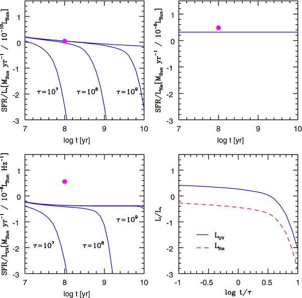
Figure 3. SFR calibrations for L*, L(Hα), Lν(UV) for t = 1–103 Myr and τ = 10–102–103 Myr. τ = ∞ corresponds to continuous SFR. Magenta hexagons show the SFR-to-luminosity ratio for continuous star-forming system in Kennicutt (1998). Top left: SFR/L*, SFR variation is fast in comparison with L* equilibration time, that is influenced by long-living low-mass stars and by reradiation of absorbed emission by dust, therefore SFR/L* drops for t/τ > 1 and is constant if τ = ∞. Top right: SFR/L(Hα), equilibration time for L(Hα) is due to the lifetime of O stars (∼3 Myr) since here τ > 10 Myr, SFR/L(Hα) is always constant. Bottom left: SFR/Lν(UV), equilibration time for UV is ∼102 Myr (life time of A stars), for τ > 102 Myr SFR/Lν(UV) is constant. Bottom right: for continuous system (τ = ∞) L*, L(Hα), and Lν(UV) show the same order of magnitude, for shorter variation (decay) timescale L* increases while L(Hα) and Lν(UV) decrease leading to mismatches up to three orders of magnitude. Our observations, in this scenario, suggest t/τ ∼ 1.
Download figure:
Standard image High-resolution imageIn contrast, any variation in the SFR is rapid compared to the equilibration time for L* for which contributions from long-living low-mass stars are significant. As the SFR drops rapidly, the decline in L* is moderated by the presence of the radiating longer-living stars. Therefore, for all τSFR/L* drops sharply when t/τ > 1. Even for continuous star formation (τ = ∞), SFR/L* declines with t, due to the continuing buildup of low-mass stars.
The UV equilibration time is ∼100 Myr, as set by the lifetimes of A-type stars. Therefore, in Figure 3, SFR/L(UV) declines with t for t/τ > 1 for τ < 100 Myr. However, for τ > 100 Myr, the variation in the star formation activity is sufficiently slow that the UV tracks the instantaneous SFR, and SFR/Lν(UV) is then a constant. In this limit, SFR/Lν(UV) = 6 × 10⁻⁷[M☉ yr−1 L−1☉ Hz−1].
Figure 3 shows the ratios Lν(UV)/L* and LHα/L* as functions of t/τ for different combination of t and τ, in the limit (τ > 100 Myr) where both Lν(UV) and (automatically) L(Hα) track the instantaneous SFR. The limit t/τ ≪ 1 is continuous star formation, and t/τ ≫ 1 is "post-burst" decaying star formation.
The following analysis is based on the comparison of various observed luminosities with the calculations presented in Figure 3. We wish to determine the values of t and τ that best match the observed L*, Lν(UV), and L(Hα). If only the LIR is considered, and viewed as a measure of L* for young (t/τ ≪ 1), dusty star-forming regions, then for our assumed IMF SFR(IR) ≃ 1.1 × 10⁻¹⁰LIR/L☉.
The post-starburst scenario implies that these objects had a higher SFR in the past, e.g., assuming the exponentially decaying star formation histories and parameters as listed in Table 3, they were typically forming stars more actively by a factor of 25 at z = 1, implying SFRs of about 60 M☉ yr−1 at that time. Their SFRs were up to 10 times faster than those estimated in normal star-forming galaxies, with an SFR–z relation of the kind (1 + z)q.
3.2. LFIR Measurements
The PACS FIR observations provide good estimates of LIR, and hence of the total stellar luminosities, L*, in the dusty star-forming regions. They give robust estimates of the SFRs in the optically obscured regions of the host galaxies for the entire galaxy and are not affected much by source geometries or central AGNs. For galaxies with detections in both PACS bands, we find the best-fitting template from the Chary & Elbaz (2001) SED library. The library includes 105 templates with gradual variations in the FIR and represents many types of local star-forming galaxies. To derive the errors on LIR, we repeat the fitting multiple times while adding noise to the fluxes, distributed normally according to the flux errors. The standard deviation of the many LIR derived in this process is taken as the error on the best-fitted LIR.
A collection of fits is shown in Figure 4. As a consistency check, we also show the 24 and 70 μm Spitzer-based luminosities when available. Even though they were not used in the fitting, in most cases Spitzer luminosities are consistent with the best selected template, confirming that the FIR-fitted templates are indeed close to the observed SEDs even at shorter wavelengths. This also suggests that AGN contributions to the 24/(1 + z) μm luminosities are small. Thus, the MIR luminosity in most of our PACS-detected LINERs is not dominated by a central AGN "obscuring torus."
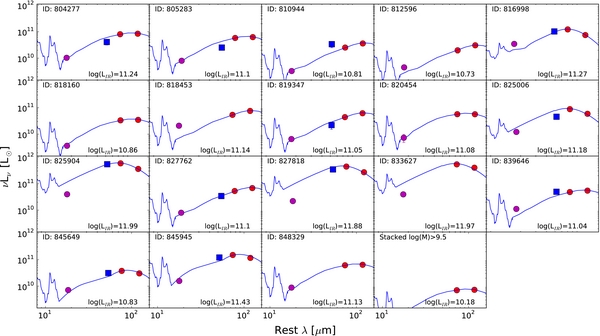
Figure 4. SED fittings of Herschel-detected LINERs in both the 100 μm and 160 μm PACS bands. Also shown are the available 70 μm and 24 μm Spitzer observations. The SED fits use only the PACS observations.
Download figure:
Standard image High-resolution imageFor galaxies detected in one band only, we experimented with relationships of the type LIR = a + blog L(λ), where λ refers to the detection band. Such approximations have been used successfully in several earlier studies, e.g., Symeonidis et al. (2008). Given the nature of our sources, for single-band detections, we prefer to estimate LFIR assuming the L(160 μm)/L(100 μm) ratio is comparable to the mean ratio of 1.975 in our sample. The calculated mean does not include the three brightest objects in our sample, 825904, 827818, and 833627, which have ULIRG-type luminosities of approximately 1012 L☉.
We attempted to estimate the dust temperature in LINERs with measurements in both PACS bands. For these sources, we measured F(100 μm)/F(160 μm) and compared it with the FIR luminosity. This is shown in Figure 5. The diagram can be compared with another sample of non active galaxies at a similar redshift, e.g., those in Hwang et al. (2010). As shown in the diagram, about 70% of our sources are "redder" than the z ∼ 0.3 in Hwang et al. (2010). Using the IR color, we estimated a single dust temperature assuming gray body emitters with an emissivity index of γ = 1.5 (see Gordon et al. 2010 for discussion and a justification of the method). The dust temperatures obtained in this way span a small range, from 24 K to 38 K. The more IR-luminous sources seem to have hotter dust, but this correlation does not appear statistically significant. The three ULIRGs in the sample show temperatures that are significantly above the mean (33 K, 34 K, 35 K) in agreement with known trends found in other samples.
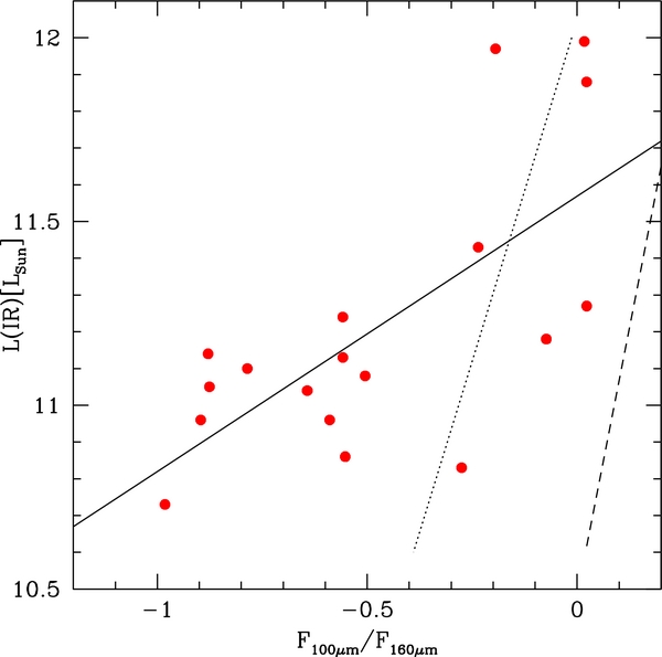
Figure 5. L(FIR) vs. IR color, F(100 μm)/F(160 μm) for 19 LINERs with 100 μm and 160 μm PACS observations. The solid line is a linear fit. The dashed and the dotted lines show similar data for non active galaxies in Hwang et al. (2010). The dashed line is the derived median IR color for objects at z = 0.3 and the dotted line is the lower limit of this group.
Download figure:
Standard image High-resolution image3.3. Lν(UV) Measurements
As explained, we used the observed FUV and NUV fluxes to calculate the spectral slope β and the (rest) 1528 Å luminosity Lν(UV). This has been done for sources with z < 0.41. The limit on the redshift is due to the short-wavelength side of the FUV band that, otherwise, includes part of the dropping stellar continuum below about 950 Å rest wavelength, the Lyman break and the Lyα absorption line. Another uncertainty in the value of β is the possible contribution of the Lyα emission line to the FUV flux. We also compared the β-based extinction estimates with the E(B − V) estimates obtained from the global (i.e., entire galaxy) SED fits (see Section 3.5 below). The SED fit procedure allows reddening by galactic-type extinction of up to E(B − V) = 0.5 mag. The values obtained in this way are considerably smaller than the value derived with the β method.
IRX, the ratio between the IR and the FUV fluxes, is a measure of extinction because it relates the dust-absorbed UV flux to the reprocessed IR flux. Meurer et al. (1999) found an empirical relationship between β and IRX in galaxies at z ∼ 3 and Seibert et al. (2005) applied the same relation to a sample of local galaxies. Such an approximation is appropriate assuming the IR and the extincted FUV arise from the same regions. We do not find a similar relationship in our LINER sample. On the contrary, we found a weak tendency of IRX to decrease in most obscured sources with highest β (see Figure 6). The reasons may be uncertainties in deriving β, the presence of a nuclear AGN source in some of the objects, or in inaccurate FUV modeling.
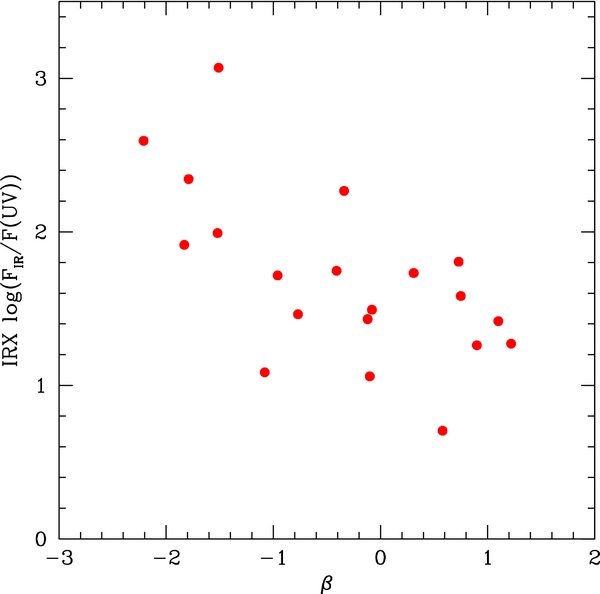
Figure 6. β vs. IRX = log (FIR/F(UV)).
Download figure:
Standard image High-resolution image3.4. L(Hα) Measurements and Reddening Estimates
In analyzing the Hα observations, we considered two alternatives: most of the Balmer line emission is produced in star-forming H ii regions or in AGN photoionized gas.
For star formation, we estimate the intrinsic Hα flux for the entire galaxy assuming that H ii regions outside of the 1'' zCOSMOS slit contribute in proportion to the surface area of the galaxy covered by the aperture. We used an estimate based on the measured iAB mag inside the slit and for the entire galaxy (zCOSMOS project; A. Bongiorno 2011, private communication). Visual inspection suggests that the B- and i-band images have similar dimensions, confirming that the i-band magnitudes provide reasonable measures of the relative fluxes emitted by early-type stars inside and outside the slit.
We apply a standard galactic (screen) extinction correction using the observed Balmer-decrement Hα/Hβ to estimate the intrinsic Hα flux within the spectroscopic aperture. We assume that the derived extinction correction factors also apply to the extrapolated estimates for the Hα emission outside the slit. The extinction corrections are uncertain because of the relatively low S/N, the weakness of the Hβ line, and the severe blending of Hβ with stellar features next to the line. For many objects, the measured Hα/Hβ ratios are below the case-B value of 2.8. For these objects, we assume zero extinction.
We have also experimented with the correction suggested by Calzetti et al. (2007) for young (continuous) star-forming regions,

where L(24 μm) is the 24 μm (dust) luminosity. The value of L(Hα)corr obtained from Equation (3) is larger by a factor of ∼10 compared to the one obtained from the observations using the Hα/Hβ-based reddening. This may indicate that a screen model is not appropriate for the star-forming regions (Bell 2003; Koyama et al. 2010; Villar et al. 2008, 2011) or a basic flow in estimating L(Hα) from the narrow slit observations.
We did not intend to study deeply SFR estimation based on Hα and UV measurements because of their uncertainty, as we said above.
3.5. Optical–MIR SED Fitting and Stellar Mass Determination
All 97 LINERs in our sample also have broadband photometric observations ranging from the U band to the 24 μm mid-IR. These data are presented in Bongiorno et al. (2010), who fit the optical to mid-IR spectral SEDs, yielding photometric estimates of the galaxy stellar masses. In these fits, the resulting system ages are large, ≳ 109 yr, and significantly greater than the inferred star formation decay times. Furthermore, extinction corrections are small. Thus, the optical–MIR SEDs are probing the predominantly unobscured and evolved stellar populations that comprise the bulk stellar mass of the LINER host galaxies. The stellar masses have been computed using the two-component SED fitting technique described in Bongiorno et al. (2012) and are listed in Table 2. We note that the stellar bolometric luminosities L* inferred from the optical–MIR SED fitting are comparable (within a factor ∼2) to the IR luminosities inferred from the PACS observations.
Table 2. Luminosities
| ID | LIR | LIRa | L(Hβ) | L(AGN)b | L(UV) | M* |
|---|---|---|---|---|---|---|
| (L☉) | (L☉) | (L☉) | (L☉) | (L☉) | (M☉) | |
| 804277 | 11.24 | 11.22 | 6.87 | 10.62 | 9.49 | 10.967 |
| 805283 | 10.96 | 10.96 | 6.93 | 10.68 | 9.53 | 10.977 |
| 810944 | 10.96 | 10.69 | 8.95 | 12.70 | 8.62 | 11.18 |
| 812596 | 10.73 | ... | 8.11 | 11.85 | 9.67 | 10.781 |
| 816998 | 11.27 | 11.56 | 7.55 | 11.30 | ... | 10.29 |
| 818160 | 10.86 | ... | 5.89 | 9.64 | 9.44 | 10.67 |
| 818453 | 11.14 | ... | 5.76 | 9.51 | ... | 9.11 |
| 819347 | 11.05 | 10.71 | 7.21 | 10.96 | ... | 11.033 |
| 820454 | 11.08 | ... | 6.58 | 10.33 | 9.36 | 11.028 |
| 825006 | 11.18 | 10.97 | 7.21 | 10.96 | 9.19 | 10.891 |
| 825904 | 11.99 | 11.94 | 6.92 | 10.67 | 9.72 | 10.368 |
| 827762 | 11.10 | 11.00 | 7.84 | 11.59 | 9.83 | 10.941 |
| 827818 | 11.88 | 11.78 | 7.49 | 11.24 | 8.81 | 10.7 |
| 833627 | 11.97 | ... | 7.45 | 11.20 | 9.38 | 11.441 |
| 839646 | 11.04 | 11.12 | 6.78 | 10.53 | ... | 10.915 |
| 845649 | 10.83 | 11.03 | 6.99 | 10.74 | 9.34 | 10.736 |
| 845945 | 11.43 | 11.51 | 7.67 | 11.42 | 9.63 | 10.804 |
| 848329 | 11.13 | ... | 6.94 | 10.69 | 9.55 | 11.077 |
| 818456 | 10.83 | ... | 6.32 | 10.07 | ... | 9.46 |
| 827400 | 10.74 | ... | 7.33 | 11.08 | 9.01 | 10.2 |
| 834427 | 11.02 | ... | 6.81 | 10.56 | ... | 9.723 |
| 838271 | 11.09 | 11.01 | 6.97 | 10.72 | ... | 10.39 |
| 804573 | 10.45 | ... | 6.90 | 10.65 | ... | 10.895 |
| 808018 | 10.31 | ... | 6.77 | 10.52 | 9.05 | 10.967 |
| 812330 | 10.91 | ... | 7.42 | 11.17 | ... | 9.93 |
| 818225 | 10.42 | ... | 6.31 | 10.06 | 8.96 | 10.722 |
| 819241 | 10.86 | ... | 6.15 | 9.90 | ... | 9.27 |
| 819596 | 10.96 | ... | 6.27 | 10.02 | ... | 9.19 |
| 823616 | 10.39 | ... | 6.72 | 10.47 | 9.69 | 10.077 |
| 830317 | 10.87 | ... | 6.78 | 10.53 | 8.96 | 10.787 |
| 832130 | 10.55 | ... | 6.39 | 10.14 | ... | 10.144 |
| 832902 | 10.93 | ... | 7.13 | 10.88 | 9.85 | 10.074 |
| 833279 | 11.00 | ... | 6.49 | 10.24 | ... | 10.02 |
| 842079 | 10.81 | ... | 6.99 | 10.74 | ... | 10.108 |
Notes. aLIR estimated by Kartaltepe et al. (2010). bL(AGN) estimated as in Netzer (2009).
Download table as: ASCIITypeset image
The SFRs derived from the optical–MIR SED fitting rely on the UV emission measurements scaled up by the dust correction factor computed using the full SED. We find that the derived values of instantaneous SFRs for the evolved populations are ∼1 M☉ yr−1, significantly smaller than the ∼10 M☉ yr−1 inferred from the FIR, assuming that the FIR is tracing continuous star formation in young star-forming regions.
To summarize, there are two distinct possibilities. Either (1) the FIR traces young (steady) star-forming regions for which SFR/LIR ≃ 10−10[M☉ yr−1L−10☉] depending only on the assumed IMF. The very different results obtained from the SED fitting could then be due to large obscuration of the H ii regions where most of the SF activity is taking place, and which are optically thick to the optical–MIR radiation. Such regions contribute little, if anything, to the bands used in the SED fitting process. Or (2) the FIR is reradiated luminosity from the evolved post-burst population for which SFR/LIR is declining and depends on the system age t and decay timescale τ, as inferred from the SED fitting and Hα and UV luminosities. The difficulty here is the large amount of dust, and its distribution through the galaxy, necessary to explain the high LFIR. The inferred SFRs for both options are listed in Table 3 together with the values of t and τ for the post-burst decay model. The value of M* obtained from the SED fit is basically independent of the two assumptions and hence we use it in the following analysis.
Table 3. Star Formation Rates
| ID | SFR(IR)a | tb | τb | SFR(IR) τ = ∞ | SFR(Hα)c | SFR(Hα)d |
|---|---|---|---|---|---|---|
| (M☉ yr−1) | (103 Myr) | (103 Myr) | (M☉ yr−1) | (M☉ yr−1) | (M☉ yr−1) | |
| 804277 | 2.68 | 7.00 | 2.00 | 17.38 | 1.46 | 0.36 |
| 805283 | 2.75 | 7.00 | 2.00 | 9.12 | 0.47 | 0.17 |
| 810944 | ... | ... | ... | 9.12 | 222.29 | 52.80 |
| 812596 | 1.99 | 9.00 | 3.00 | 5.37 | 14.95 | 7.59 |
| 816998 | ... | ... | ... | 18.62 | 3.06 | 1.47 |
| 818160 | 0.50 | 9.00 | 2.00 | 7.24 | 0.12 | 0.04 |
| 818453 | 0.13 | 2.00 | 0.60 | 13.80 | 0.06 | 0.03 |
| 819347 | 1.34 | 5.00 | 1.00 | 11.22 | 2.59 | 0.97 |
| 820454 | 1.33 | 5.00 | 1.00 | 12.02 | 0.57 | 0.20 |
| 825006 | 2.56 | 9.00 | 3.00 | 15.14 | 1.49 | 0.65 |
| 825904 | ... | ... | ... | 97.72 | 0.73 | 0.37 |
| 827762 | 2.52 | 7.00 | 2.00 | 12.59 | 11.98 | 4.09 |
| 827818 | 0.003 | 3.00 | 0.60 | 75.86 | 3.87 | 1.85 |
| 833627 | 2.94 | 9.00 | 2.00 | 93.33 | 5.06 | 1.68 |
| 839646 | 2.38 | 7.00 | 2.00 | 10.97 | 0.53 | 0.18 |
| 845649 | 1.58 | 7.00 | 2.00 | 6.76 | 1.56 | 0.58 |
| 845945 | 1.84 | 7.00 | 2.00 | 26.92 | 7.13 | 2.82 |
| 848329 | 1.49 | 5.00 | 1.00 | 13.49 | 2.22 | 0.52 |
| 818456 | ... | ... | ... | 6.75 | 0.09 | 0.04 |
| 827400 | ... | ... | ... | 5.50 | 2.72 | 1.28 |
| 834427 | 1.73 | 3.00 | 3.00 | 10.54 | 0.54 | 0.29 |
| 838271 | 0.71 | 7.00 | 2.00 | 12.40 | 2.16 | 0.56 |
| 804573 | 0.84 | 9.00 | 2.00 | 2.83 | 1.11 | 0.48 |
| 808018 | 0.0025 | 7.00 | 0.60 | 2.05 | 0.55 | 0.35 |
| 812330 | ... | ... | ... | 8.14 | 2.31 | 1.58 |
| 818225 | 0.20 | 4.00 | 0.60 | 2.64 | 0.30 | 0.12 |
| 819241 | 9.95 | 0.26 | 30.00 | 7.19 | 0.35 | 0.05 |
| 819596 | ... | ... | ... | 9.18 | 0.25 | 0.09 |
| 823616 | 1.24 | 2.00 | 0.60 | 2.48 | 1.13 | 0.32 |
| 830317 | 2.01 | 9.00 | 3.00 | 7.43 | 0.98 | 0.36 |
| 832130 | 0.47 | 4.00 | 1.00 | 3.57 | 0.31 | 0.13 |
| 832902 | 3.09 | 2.00 | 1.00 | 8.56 | 1.86 | 0.81 |
| 833279 | ... | ... | ... | 10.01 | 0.25 | 0.17 |
| 842079 | 11.91 | 1.60 | 15.00 | 6.43 | 0.69 | 0.26 |
Notes. aSFR only for LINERs with line S/N > 3. bt, τ are obtained as in Section 3.1. cHα corrected for extinction and aperture. dHα corrected only for extinction.
Download table as: ASCIITypeset image
We have used our data to construct two SFR versus M* diagrams (Figure 7) in order to check analogies between the host galaxies of our sample of LINERs and star-forming galaxies. On the SFR versus M* diagram, star-forming galaxies form a well-defined "main sequence" (MS; see Noeske et al. 2007). For reasons discussed below, we consider the SED derived M* to represent well the stellar mass in both cases. Both diagrams show SFRs based on the measured LFIR which is the one least affected by the observational uncertainties. The diagram includes 34 LINERs with at least one Herschel detection and two stacks representing the remaining 40 sources with Herschel upper limits, see Section 2.2. The uncertainties on the masses are obtained from the SED fitting procedure and reflect only the photometric uncertainties. Uncertainties on SFRs are only observational and reflect the uncertainty on the PACS photometry. They do not include the uncertainty in FIR SED fitting. The uncertainties on the stacked data are due to the scatter between sources in these groups and reflect their variance (due to both intrinsic and observational errors).
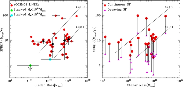
Figure 7. Left panel: SFR vs. stellar mass for the LINER sample. Plotted are 34 objects detected by Herschel with σ > 3, red circles, and stacked point, the green pentagon and the cyan hexagon. Black circles show the average of SFRs in mass bins of eight objects. The error bars represent the standard deviation in the bin. Right panel: SFR vs. stellar mass for Herschel-detected objects considering two possibilities: as continuous SF galaxies (red circles) and post-starburst systems with t and τ as in Section 3.1 (magenta triangles).
Download figure:
Standard image High-resolution imageThe SFR versus stellar mass relations in the two diagrams are very different. For model (1; left panel), our sample lies along the MS for star-forming galaxies. This is illustrated by the two diagonal lines that represent the mean MS at two redshifts, z = 0.1 and z = 1 from Dutton et al. (2010) and references therein. Most of the detected LINERs lie close to the expected location of the z = 0.3 MS with the three ULIRGs well above it. There is a clear tendency for the lower M* sources (those with M* < 109.5) to have smaller SFR. The consistency with the MS, in combination with the HST images that show that most of the galaxies in our sample are spirals, is evidence that the FIR is in fact tracing young embedded star-forming regions, with large inferred SFRs ∼10 M☉ yr−1. Because of the large scatter for the mean values of the SFR(IR), we have calculated the average masses and SFR(IR) of the detected sources divided in four bins of eight objects with similar stellar mass. We also included in the mean the stack with higher M*, considering it as a single source. Consistent with the general result, the three bins including objects with higher stellar mass lie in the MS region, while the smaller mass bin lies above that region.
The right-hand panel of Figure 7 shows the positions of our galaxies, assuming model (2) for which the derived SFRs correspond to post-burst systems with t and τ estimated by our SED fitting procedure. The sources are well below the two MS lines as expected for passive galaxies with declining SFRs. More discussion of these findings is given in Section 4.
4. DISCUSSION
4.1. Comparison with Other Samples of SF Galaxies
Our sample of LINER host galaxies shows clear discrepancies between various SF indicators that are based on the UV continuum, the Balmer emission lines, and the FIR emission, assuming continuous star formation. Such discrepancies have been found in previous studies. For example, Rigopoulou et al. (2000) estimated SFR(Hαobs) up to an order of magnitude smaller than SFR(IR) in their 15 μm selected sample of starburst galaxies at z > 0.4. The typical SFR(IR) in their sample is somewhat larger than the one we find in the LINER sample using the Herschel-based estimates. However, their SFR(Hαobs) is about 10 times larger than ours. Cardiel et al. (2003) found SFR(Hα) > SFR(UV) in a sample (z ∼ 0.4 and 0.8) with a mean SFR(Hα) larger than ours by about a factor six. They also found that SFR(Hα) consistently underestimates the SFR and the discrepancy is larger for higher LIR for a continuous burst. In a sample of 15 μm selected LIRGs at 0.1 < z < 0.8, Flores et al. (2004) obtained SFR(IR) comparable to ours for low-z galaxies. However, their SFR(Hα) is considerably larger than ours and is in better agreement with LIR. These authors suggested emission from two different regions in the galaxy with a different amount of obscuration, similar to our case (1) (see Section 3). Finally, Liang et al. (2004) obtained the same results of Flores et al. (2004) in their 15 μm selected galaxy sample at z < 1.
A general discussion of the various methods and the merit of extinction correction methods is given in Wuyts et al. (2011). These authors used Herschel-PACS data and compared them with various other observations mostly at high redshifts. They discussed the way UV-, Hα-, and FIR-based estimates can be reconciled by using proper dust attenuation correction factors. They find clear evidence for deviation of the various method at SFR > 100 M☉ yr−1, but the sample is not complete enough at low redshift and low SFR to compare with the present LINER sample.
The main conclusion of the above comparison is that L(Hα) is problematic and tends to underestimate the SFR, even in sources (LIRGs or high SFR high-z galaxies) where the assumption of a continuous burst is justified and it is not possible to apply to a decaying scenario.
4.2. Color Morphology and SF in LINER Host Galaxies at z = 0.3
We adopt the morphology based on HST images as listed in the IPAC Archive.9 This reference classifies 24 sources as spirals, seven as ellipticals, and three as irregular galaxies (see Table 1). Additional inspection of the HST images suggests that some, perhaps even all, sources classified as elliptical galaxies may in fact be disky systems. This supports the idea that most of our sources contain H ii regions that are likely to be outside the 1'' slit (assuming it was placed across the centers of these galaxies).
We have also looked at the color of the sources as derived from the multi-band photometry. Most objects have reddish colors and are similar in this respect to the much larger COSMOS galaxy sample discussed in detail in Bongiorno et al. (2010). This again is consistent with a combination of old stellar population and highly obscured H ii regions in the disk. The alternative is that the red color is due to reddening and extinction. Unfortunately, our broadband photometry which lacks information on the very short wavelengths is insensitive to such reddening.
4.3. SFRs and AGN Luminosity in Local and z = 0.3 LINERs
We now consider the possibility that most of the line emission inside the 1'' slit is from AGN-ionized gas. We can then compare the AGN and the SF luminosities to those observed in local LINERs. Our estimated bolometric AGN luminosities, L(AGN), are based on the approximation given in Netzer (2009),
where L(Hβ) is the galactic extinction corrected Hβ luminosity. A more accurate estimate of L(AGN) in LINERs is based on a combination of L([O iii] λ5007) and L([O i] λ6300) (Netzer 2009). This cannot be used in the present case, since the weaker [O i] λ6300 line is not observed in most of the z = 0.3 LINERs. We do not correct the Balmer line flux for the aperture size because we consider only nuclear emission-line regions (this assumption was also used in Bongiorno et al. 2010). Given this approximation, we find that the AGN bolometric luminosity in our sample is between 1042.6 and 1044.9 erg s−1.
Considering that all the LIR is due to SF, and thus LSF = LIR, we compared L(AGN) and LIR in our LINER sample with those of the local (z ⩽ 0.01) LINERs studied by Ho et al. (1997) using only objects classified as type-II LINERs. For most of the local LINERs, we can use the IRAS 60 μm and 100 μm fluxes and the expression provided in Sanders & Mirabel (1996),

where F(60 μm) and F(100 μm) are the fluxes in the relevant IRAS bands to obtain LSF. We do not include the IRAS 12 and 25 μm fluxes since they may be influenced by warm AGN-heated dust. We also calculated L(AGN) for all these sources using the same method as for the Herschel-detected LINERs. The resulting LIR versus L(AGN) for the two samples is shown in Figure 8. The diagram also shows a line indicating the location of AGN-dominated objects from Netzer (2009). Local LINERs show considerably lower L(AGN) and LSF and the two samples form a continuous sequence in both properties.

Figure 8. L(AGN) as in Netzer (2009) vs. LIR in our sample and in Ho et al. (1997). The L(AGN) of the stacked sources is the average L(AGN) of the binned sources and the error bars are the standard deviation from the mean. The solid line is the empirical relationship for AGN-dominated sources from Netzer (2009).
Download figure:
Standard image High-resolution image
There are several possible reasons for the very different properties of the two groups. First, in local LINERs, the line emission is from the very nuclear regions of the galaxy which are much smaller, in terms of physical size, than the regions covered by the 1'' slit in our z ∼ 0.3 sample. Second, most of the z = 0.3 LINERs have not been detected by Herschel and our comparison is based on objects that were detected and hence show the largest LSF. Third, there may well be a population of local (z < 0.1) LINERs with higher LSF that have not been studied, systematically, with sensitive FIR instruments, maybe because the volume probed by local surveys is too small to contain them. Finally, there may well be a real evolution in the AGN and SF properties of LINER host galaxies between z = 0 and z ∼ 0.3. To test this idea, one needs a systematic study based on FIR observations of LINERs over a large redshift range. The gap between the two samples may also be due to a selection effect, because the fainter FIR sources are not included in the diagram. To test this, we plotted on this diagram L(AGN) versus L(IR) for the two stacks shown in Figure 7. If M* > 109.5 M☉, then the stacked source lies anyway in the z ∼ 0.3 LINERs region. For smaller M*, the stacked source descends into the gap region, but its IR measurement is only an upper limit, which may affect the correlation.
4.4. Revised Diagnostic Diagrams for LINERs
Our new FIR observations and stellar evolution analysis suggest that LINER-like spectra from the inner parts of early-type galaxies are not necessarily related to old stellar populations. Obscuration in the nucleus and the disk can hide much of the line emitting gas (Sturm et al. 2006; Dudik et al. 2009), and post-starburst system, as discussed here, (Section 4.2) can result in large LFIR. This raises several general questions regarding the usefulness of some of the commonly used line diagnostics in galaxies showing high LIR and obscuration.
Spectroscopic studies of LINERs in the local universe, e.g., SDSS LINERs, indicate low extinction as judged from the observed Hα/Hβ line ratio (e.g., Kauffmann et al. 2003). These observations refer to the inner 3'' part of the host galaxy (the diameter of the SDSS fiber used for spectroscopy). In contrast, highly ionized type-II sources show a clear correlation of extinction with SFR as measured by the Dn4000 Å index and by GALEX UV observations (e.g., Salim et al. 2007 and references therein). The mean Hα/Hβ in our z ≃ 0.3 sample is also small (about 50% of the Herschel-detected LINERs have Hα/Hβ <2.8, i.e., consistent with no reddening), yet LIR is high, which suggest high obscuration in H ii regions mostly outside the 1'' slit. Thus, the spectroscopic definition of LINERs, which is based on the observed [O iii]/Hβ and [N ii]/Hα line ratios, can critically depend on the aperture size and the H ii regions distribution, and extinction, in the disk. We suspect that larger aperture spectroscopic observations of our LINERs will reveal composite LINER/H ii spectra.
The general issue of composite versus "pure" AGN spectra has been discussed in various papers, most recently by Wild et al. (2010). This paper assesses the fraction of high ionization AGNs in three groups, SF galaxies, composite SF–AGN objects, and pure AGNs. We suggest that our LINER classified objects would be considered composite SF–LINER objects had they been observed with larger spectroscopic aperture. A complex geometry can contrive to mix LINERs and H ii regions and confuse the standard spectroscopic diagnostics.
Another possibility that was already mentioned is related to extreme obscuration in compact, luminous H ii regions. The obscuration in such H ii regions can be so large that the standard use of the Hα/Hβ line ratio to correct for extinction may not be valid. One must therefore consider the possibility that "pure" LINERs, with emission lines that are excited exclusively in AGN photoionized gas, cannot be unambiguously identified in galaxies with large SFRs. The temperatures that we estimated for those galaxies with two PACS detections do not seem high enough to be related to compact H ii regions, but their measurements suffer from uncertainty due to observations and modeling, so that we cannot exclude the existence of heavily obscured H ii regions.
5. CONCLUSIONS
We present the first systematic study of the FIR properties of LINERs at z ∼ 0.3. The sample includes 97 LINERs from the first release of zCOSMOS and their emission-line properties have been studied by Bongiorno et al. (2010). The main findings of our work are as follows.
- 1.Thirty-four of the sources have σ > 3 detections in at least one Herschel/PACS band. The mean LFIR in this group is about 1044.5. We were able to divide the remaining sources in two groups according to their M*. Stacking sources in the first (M* > 109.5) group gave a significant mean L(IR) signal. The remaining sources with M* < 109.5 provided only upper limit.
- 2.Assuming that the FIR arises in young star-forming regions, the FIR luminosities imply typical SFRs of ∼10 M☉ yr−1.
- 3.Almost all LINERs have FUV and/or NUV GALEX detections. The UV flux is slightly larger for objects with PACS detections. However, the SFRs obtained with the UV-corrected fluxes are low compared to the SFRs inferred from the Herschel measurements, assuming the UV is produced in young star-forming regions producing the FIR.
- 4.The assumption that all the Hα line flux is due to SF was used to obtain L(Hα)-based SFRs. These are considerably smaller than the FIR-based SFRs assuming young-and-steady star formation. This may be due to the inaccuracy of the Hα and UV extinction estimates, especially since SF occurs in regions that are optically thick to the UV/Optical radiation. Alternatively, the Hα and UV may be tracing residual "post-burst" star formation in the older underlying population and may be unassociated with the ongoing star-forming regions that produce the FIR.
- 5.The assumption that all the Hα line flux is due to SF was used to study two different SF scenarios. The first assumes continuous SF in highly obscured H ii regions and the second a post-starburst decay. Both scenarios have their own shortcomings, but the first seems to agree better with the observations including the fact that the HST images of most sources show evidence for disk-type systems. Under the more favorable assumption, almost all of the Herschel-detected LINERs are situated on the MS in the SFR versus M* diagram.
- 6.All our Herschel-detected LINERs are situated above the location of local LINERs in the LSF versus L(AGN) diagram in both axes.
- 7.The present work raises the possibility that simple optical line diagnostic diagrams based on spectroscopy of the central parts of galaxies can indicate a typical LINER spectrum in cases where the host galaxy undergoes enhanced SF activity.
We acknowledge Roberto Maiolino and David Rosario for the useful comments and the DFG for support via German-Israeli Project Cooperation grant STE1869/1-1/GE625/15-1.
Footnotes
- 6
- 7
- 8
- 9
IPAC Infrared Science Archive (IRSA)—Cassata Morphology Catalog v1.1.