


ABSTRACT
The present paper provides a possible explanation for the solar wind electron velocity distribution functions possessing asymmetric energetic tails. By numerically solving the electrostatic weak turbulence equations that involve nonlinear interactions among electrons, Langmuir waves, and ion-sound waves, it is shown that different ratios of ion-to-electron temperatures lead to the generation of varying degrees of asymmetric tails. The present finding may be applicable to observations in the solar wind near 1 AU and in other regions of the heliosphere and interplanetary space.
Export citation and abstract BibTeX RIS
1. INTRODUCTION
The electron velocity distribution functions (VDFs) associated with the solar wind near 1 AU and in the upstream region of Earth's bow shock are observed to consist of thermal core plus energetic suprathermal (or halo) populations (Vasyliunas 1968; Montgomery et al. 1968; Feldman et al. 1975; Rosenbauer et al. 1976; Pilipp et al. 1987; Lin et al. 1981, 1986; Lin 1998; Fitzenreiter et al. 1990, 1998; Maksimovic et al. 1997, 2005; Ergun et al. 1998; Ogilvie et al. 1999; Pagel et al. 2007; Nieves-Chinchilla & Viñas 2008; Stverak et al. 2009). The solar wind electron VDFs are customarily modeled by the kappa distribution (Vasyliunas 1968). However, actual electron VDFs often feature highly asymmetric energetic tails such that they cannot always be fitted by a simple one-component kappa model. Examples of asymmetric halo distributions in the solar wind can be found in the papers by Pilipp et al. (1987) and Fitzenreiter et al. (1998). Gaelzer et al. (2008) also provide examples of asymmetric electron VDFs in the solar wind. Asymmetric foreshock electron VDFs can be found in the paper by Fitzenreiter et al. (1990). An excellent collection of asymmetric VDFs can be found in the paper by Nieves-Chinchilla & Viñas (2008), who analyzed data taken inside closed magnetic field structures known as magnetic clouds.
Gaelzer et al. (2008) were the first to address the issue of asymmetric electron VDFs within the context of electron acceleration by the beam-generated Langmuir turbulence. The first actual demonstration that Langmuir turbulence may lead to quasi-kappa-like VDFs by wave–particle acceleration was done by Yoon et al. (2005, 2006) and Rhee et al. (2006). By employing one-dimensional (1D) particle-in-cell simulation, Ryu et al. (2007) subsequently confirmed the above-mentioned findings, which were based on weak turbulence theory. However, the kappa-like VDFs obtained in the papers by Yoon et al. (2005, 2006), Rhee et al. (2006), and Ryu et al. (2007) were all more or less symmetric in the forward and backward directions. Gaelzer et al. (2008) built upon these findings and numerically investigated the situation when there exist counter-streaming electron beams in addition to the background core electrons. According to Gaelzer et al. (2008), suprathermal electron VDFs with varying degrees of asymmetry can be generated when judicious choices of relative beam densities and counter-propagating beam speeds are made.
The justification for considering counter-streaming electron beams may be found in situations when both footpoints of the interplanetary magnetic field line loops are located on the Sun. In such a situation, the field-aligned motion of the electrons may be characterized as counter-streaming. Sufficiently close to Earth's electron foreshock, the reflected electrons off the cross-shock electrostatic potential may coexist with the incoming solar wind electrons. Finally, counter-propagating beams can exist inside magnetic clouds. However, when asymmetric electron VDFs are detected in the fast solar wind for which no apparent connection can be made with magnetic cloud-like structure, the assumption of counter-streaming electrons may not be valid.
In the present paper, we therefore resort back to the situation where there exists only a single component of energetic (beam) electrons. We find that the role of ion-to-electron temperature ratio, Ti/Te, which has been overlooked in the paper, can be important in the final production of asymmetric electron VDFs. In earlier studies by Yoon et al. (2005, 2006), Rhee et al. (2006), Ryu et al. (2007), and Gaelzer et al. (2008), the ratio Ti/Te was not varied, but instead a small (less than unity) fixed value was adopted. This was based on the assumption that small Ti/Te is necessary for the existence of ion-sound turbulence; otherwise, the ion-sound mode suffers damping. The presence of an ion-sound wave is deemed important since it mediates the three-wave decay process, which involves two Langmuir waves and an ion-sound wave. Consequently, their existence promotes the nonlinear mode coupling. For this reason, a small value of Ti/Te was adopted in previous studies. However, the actually measured temperature ratio in the solar wind shows a considerable variation. In an early paper by Gurnett et al. (1979), one finds that Ti/Te ranges from  to
to  in the solar wind. Similar variation of Ti/Te in the range
  to
to  is also reported in the paper by Newbury et al. (1998). This implies that it is necessary to consider a range of Ti/Te when considering the electron–Langmuir turbulence interaction problem. We thus have carried out a series of numerical solutions of the equations of weak turbulence theory for a range of Ti/Te. We find that when Ti/Te is systematically varied, the resulting nonlinear processes lead to asymmetric electron VDFs even though the initial configuration consists of only one electron beam moving in the background plasma. In the rest of the present paper, we report our findings in a systematic manner.
2. THEORETICAL FORMULATION AND NUMERICAL ANALYSIS
2.1. Theoretical Equation
The theoretical framework of the present paper is the self-consistent weak turbulence equations that describe nonlinear interactions among Langmuir and ion-sound modes, as well as with the particles. In the present analysis, we resort to 1D approximation and assume that only electrostatic interaction is of importance. The equations of weak turbulence theory can be found in the papers by Yoon et al. (2006), Rhee et al. (2006), Pavan et al. (2009), and Ziebell et al. (2008, 2012). These consist of Langmuir and ion-sound wave kinetic equations and the particle (electron) kinetic equation. For the sake of completeness, we reproduce the fully 3D version of the self-consistent set of equations, although in the actual numerical computation only the 1D situation shall be considered,

where fe is the electron VDF (normalized to unity, ∫dvfe = 1) and  is the stationary ion VDF. The quantities IσLk and IσSk stand for Langmuir and ion-sound mode intensities, respectively, and are related to the total spectral fluctuating electric field energy density by

In the above σ = ±1 designates the direction of the wave phase speed, the plus/minus denoting the forward/backward direction. The quantities me and mi are electron and ion rest masses, respectively, ω2pe = 4πne2/me represents the square of the plasma frequency, and v2Te = 2Te/me and v2Ti = 2Ti/mi are the squares of electron and ion thermal speeds, respectively, Te and Ti being electron and ion temperatures, respectively. The wave dispersion relations for L (Langmuir) and S (ion-sound) waves are well known in the literature,
The quantity μk is defined by
The physical meaning of the various terms in the particle (electron) kinetic equation and the wave kinetic equations for L and S modes has already been discussed in previous papers by Yoon and his colleagues (Yoon et al. 2006; Rhee et al. 2006; Pavan et al. 2009; Ziebell et al. 2008, 2012), so we shall not repeat them in full detail, but briefly, we shall only note that those terms dictated by the resonance condition delta function δ(σωLk − k · v) or δ(σωSk − k · v) represent linear wave–particle interactions, those dictated by  or
or  stand for nonlinear wave–wave resonant interactions, and finally the term associated with δ[σωLk − σ'ωk'L − (k − k') · v] depicts nonlinear wave–particle resonance.
We have solved the set of Equation (1) in 1D approximation for an initial electron VDF given by the combination of a core Maxwellian component and a beam population, which in 1D is given by

where v2Tb = 2Tb/me is the thermal spread associated with the beam electrons. In general the beam component is not observed for quiet-time solar wind, although during impulsive events such as the type III radio bursts, the electron beam is often observed together with enhanced Langmuir turbulence and electromagnetic radiation (Lin et al. 1981, 1986). The actual presence of a field-aligned beam component is not easy to detect by experimental means, however. In the present paper, we consider an initial beam component to facilitate the excitation of Langmuir turbulence so that we may allow faster dynamical evolution. Our purpose is to compare the long-time solution, not the initial VDF, with observed VDFs, so that the choice of admittedly somewhat arbitrary initial electron beam is immaterial in the end. In the computation, we therefore assume that the ratio of electron beam speed to background thermal speed is given by Vb/vTb = 4 for all the cases considered. We also assume that the initial Gaussian thermal spread associated with the beam component is equal to the background temperature, Tb = Te.
Initial wave intensities are specified by requiring the balance of spontaneous and induced emission processes, which in 1D are specified by

In the numerical analysis there are other physical parameters that must be specified. For instance, one of the crucial parameters is the so-called plasma parameter, g = 1/nλ3De, which represents the inverse of the number of particles in the sphere of radius equal to the Debye length. Here, λ2De = Te/(4πne2) is the electron Debye length squared, Te, n, and e being the electron temperature, ambient density, and unit electric charge, respectively. For a typical solar wind near 1 AU, the electron temperature is of the order 104–105 K, and the ambient density can be as low as 1 cm−3 and can reach up to  cm−3, and sometimes even higher. When the plasma parameter g is computed on the basis of these quantities, we find that
  to
to  or so. In the present weak turbulence simulation, the finiteness of the g parameter is crucial in that if we set g = 0 exactly, then all the terms corresponding to spontaneous thermal effects vanish—the term associated with the drag coefficient A in the electron kinetic equation, the term ne2fe/π in the Langmuir wave kinetic equation, the term associated with
  in the nonlinear term of the Langmuir wave kinetic equation, and finally the term ne2(fe + fi)/π in the ion-sound wave kinetic equation. It was shown by Yoon et al. (2006) and Rhee et al. (2006) that without these terms, no suprathermal tail forms.
Often, the finiteness of the g parameter is related to the collisionality of the solar wind. Near 1 AU, it is often said that the solar wind is "collisionless." However, even though g may be small, it is nevertheless finite. The finiteness of g leads to the formation of suprathermal tails in the electron–Langmuir turbulence scenario. In the present analysis, we shall consider a slightly higher value of g than the actual observation so as to facilitate the numerical computation and to demonstrate the formation of an energetic tail within a reasonable timescale. Specifically, we shall consider g = 5 × 10⁻³. Another input parameter is the energetic-to-core electron density ratio, nb/ne. Observations of the solar wind near 1 AU and beyond show that the halo-to-core electron number density ratio is of the order  or so (Maksimovic et al. 2005; Stverak et al. 2009). From this we choose the ratio nb/ne = 10−2. We consider a range of the ratio of ion and electron temperature Ti/Te: specifically, Ti/Te = 1/15, 1/10, 1/7, 1/4, 1/2, and 1. Note that Yoon et al. (2005, 2006), Rhee et al. (2006), Ryu et al. (2007), and Gaelzer et al. (2008) all considered a fixed value of Ti/Te sufficiently less than unity. In contrast, we consider Ti/Te ranging from 1/15 to as high as 1.
2.2. Numerical Results
Figure 1 displays the electron VDFs for six different cases corresponding to (1) Ti/Te = 1/15, (2) Ti/Te = 1/10, (3) Ti/Te = 1/7, (4) Ti/Te = 1/4, (5) Ti/Te = 1/2, and (6) Ti/Te = 1, for initial input physical parameters nb/ne = 10−2, Vb/vTe = 4, and g = 5 × 10⁻³. The first two cases, namely, Ti/Te = 1/15 and Ti/Te = 1/10, show that over a long computational period (up to ωpet = 2 × 10⁴), the initial core plus beam system evolved to a system composed of the core population, which did not undergo much change, plus a prominent pair of quasi-symmetric tail populations that emerged gradually over time. For cases (3) and (4), for which Ti/Te = 1/7 and Ti/Te = 1/4, respectively, it can be seen that the tail formation is slightly reduced over the same time period when compared with the previous two cases. Note that the two cases appear nearly identical, which shows that the variation on Ti/Te in the range Ti/Te = 1/7 to 1/4 appears to have little impact on the change in the dynamics. It can also be seen that the forward and backward components are slightly asymmetric, with the backward tail slightly more prominent than the forward tail. The case of Ti/Te = 1/2, on the other hand, shows that it definitely has more influence on the change in the dynamics. Specifically, it can be seen that the asymmetry has increased when compared with the previous two cases. The final case of Ti/Te = 1 shows a further increase in the asymmetry. From the results shown in Figure 1, it is clear that varying Ti/Te affects the degree of asymmetry—the higher the ratio, the more prominent is the asymmetry.
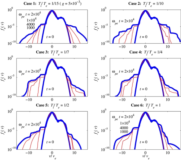
Figure 1. Electron VDFs for six different cases corresponding to (1) Ti/Te = 1/15, (2) Ti/Te = 1/10, (3) Ti/Te = 1/7, (4) Ti/Te = 1/4, (5) Ti/Te = 1/2, and (6) Ti/Te = 1, for initial input physical parameters nb/ne = 10−2, Vb/vTe = 4, and g = 5 × 10⁻³.
Download figure:
Standard image High-resolution imageIn order to understand the physical reason why the change in the ion-to-electron temperature ratio should have such a definite impact on the formation of the asymmetric tail distribution, we now plot the Langmuir wave intensity as a function of normalized wave number kvTe/ωpe and normalized time ωpet. For the case of low Ti/Te = 1/15, one may observe that, after an initial excitation of bump-in-tail instability near kvTe/ωpe ∼ 1/4, the subsequent evolution of the spectrum involves the backscattering to negative k mode and the formation of the so-called Langmuir condensate near small k. It can be seen that the wave spectrum is rather smooth in k space, and near the end of the temporal plotting range, ωpet = 104, the level of Langmuir wave intensity in the positive (k > 0) and negative (k < 0) wavenumber space is comparable in strength.
For the next three cases, Ti/Te = 1/10, 1/7, and 1/4, one can see that the spectrum develops fine structure in k space, and the backward Langmuir wave component shows increasingly higher intensity as the case moves from Ti/Te = 1/10, to Ti/Te = 1/7, to Ti/Te = 1/4. This explains why the negative v tail becomes more and more prominent. Note that the cases of Ti/Te = 1/7 and Ti/Te = 1/4 are nearly identical, but upon careful examination, one can discern small but noticeable differences in the fine-structure spectrum. Finally, the trend of increasing negative k mode intensity continues as the case moves to Ti/Te = 1/2 and to Ti/Te = 1. It is interesting to note that for Ti/Te = 1 the fine structure has somewhat dissipated and the Langmuir wave spectrum again looks rather smooth in k space.
To further understand the dynamics, let us examine the wave spectrum associated with the ion-sound mode. Shown in Figure 3 is the plot of ion-sound spectral intensity in the same format as Figure 2. For the first case of Ti/Te = 1/15, for which the linear theory predicts that ion-sound damping should be small, it can be seen that the ion-sound turbulence is generated via three-wave decay instability, in both the forward and backward propagation directions. The strong excitation of S mode via the decay process takes the wave energy out of L mode, and as such the corresponding Langmuir wave spectrum shown in Figure 2 case (1) indicates relatively low L mode wave energy when compared to other cases. Moving on to case (2) where Ti/Te = 1/10, for which the Landau damping rate should increase slightly, it can be seen from Figure 3 case (2) that the ion-sound mode intensity has decreased somewhat when compared to case (1). Also, note the appearance of fine structure in the S mode spectrum. This is consistent with similar fine structure in the corresponding L mode. As Ti/Te increases, Figure 3 cases (3)–(6) show steady decline in the S mode wave intensity. Note that in the final case (6), for which Landau damping of S mode should be the highest among the cases considered, the fine structure in the spectrum has decreased, which is again consistent with the corresponding L mode spectrum.
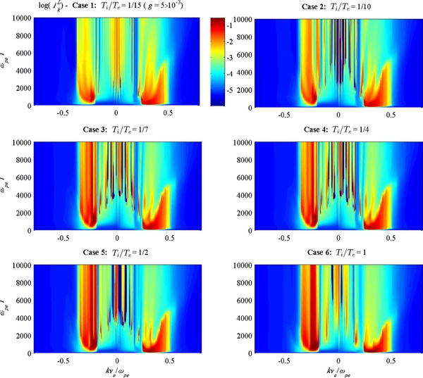
Figure 2. Time evolution of the Langmuir wave intensity for six different cases corresponding to (1) Ti/Te = 1/15, (2) Ti/Te = 1/10, (3) Ti/Te = 1/7, (4) Ti/Te = 1/4, (5) Ti/Te = 1/2, and (6) Ti/Te = 1, for initial input physical parameters nb/ne = 10−2, Vb/vTe = 4, and g = 5 × 10⁻³.
Download figure:
Standard image High-resolution image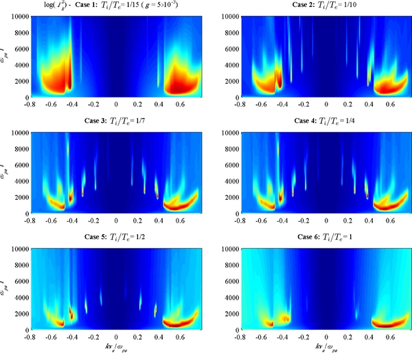
Figure 3. Time evolution of the ion-sound wave intensity for six different cases corresponding to (1) Ti/Te = 1/15, (2) Ti/Te = 1/10, (3) Ti/Te = 1/7, (4) Ti/Te = 1/4, (5) Ti/Te = 1/2, and (6) Ti/Te = 1, for initial input physical parameters nb/ne = 10−2, Vb/vTe = 4, and g = 5 × 10⁻³.
Download figure:
Standard image High-resolution image
We have also repeated the same set of calculations for lower values of the g parameter. As expected, the formation of the tails in the case of lower values of g was found to be less pronounced over the same computational timescale. Upon examining the Langmuir wave and ion-sound mode spectral intensities in the case of lower values of g, we found that the overall spectral features were consistent with the case of g = 5 × 10⁻³. However, the important consequence of a lower g parameter seems to be the delay in the formation of the energetic tail population. We have not shown numerical examples in order to avoid repetitions. However, it is important to note that as long as a finite g value is chosen, eventually the energetic electron population will be generated by the Langmuir turbulence process. As a matter of fact, Yoon (2011, 2012a, 2012b) and Yoon et al. (2012) showed that the balance of spontaneous and induced processes will always produce the energetic tail population in the time-asymptotic state, t → ∞, regardless of the value of g.
3. CONCLUSIONS AND DISCUSSION
The present paper puts forth a possible explanation for the observed electron VDFs in the solar wind near 1 AU that shows varying degrees of asymmetry associated with the energetic suprathermal tail population. In a recent paper, Gaelzer et al. (2008) proposed a mechanism for the generation of asymmetric suprathermal electrons. In their work, a pair of initially counter-streaming energetic but tenuous electron beam populations is hypothesized. On the basis of such an initial configuration, they demonstrated that a wide variety of asymmetric energetic tail distributions result. However, the existence of counter-streaming electrons may be realized only under special situations such as near Earth's collisionless shock or inside magnetic clouds.
In contrast to Gaelzer et al. (2008), the present paper assumes a single beam moving along the field line in the background of core Maxwellian electrons, which is probably more applicable to a general situation. The new and interesting finding in the present work is that the varying ratios of proton to electron temperatures, Ti/Te, play a crucial role in determining the degree of asymmetry in the electron VDF. The observation of Ti/Te in the solar wind (Gurnett et al. 1979; Newbury et al. 1998) indicates that Ti/Te can vary from  to order unity. We have thus varied Ti/Te in a similar range and found that the resulting nonlinear mode coupling between Langmuir and ion-sound turbulence dictates how the asymptotic electron VDF should form. We find that in general, low Ti/Te leads to a more symmetric VDFs, while higher Ti/Te leads to an asymmetric electron VDF. However, this conclusion is based on the variation of Ti/Te, while other parameters such as the beam density and beam speed are fixed. Consequently, further more systematic parametric study is necessary. The present preliminary finding that lower Ti/Te correlates to more symmetric VDFs and vice versa can be validated from observations, which we leave as a task for the observation and data analysis community.
The research at the University of Maryland was supported by NSF Grant AGS0940985. The research carried out at Kyung Hee University, Korea, was supported by WCU Grant R31-10016 from the Korean Ministry of Education, Science, and Technology.