
Abstract
PET (positron emission tomography) with its high sensitivity in combination with MRI (magnetic resonance imaging) providing anatomic information with good soft-tissue contrast is considered to be a promising hybrid imaging modality. However, the integration of a PET detector into an MRI system is a challenging task since the MRI system is a sensitive device for external disturbances and provides a harsh environment for electronic devices. Consequently, the PET detector has to be transparent for the MRI system and insensitive to electromagnetic disturbances. Due to the variety of MRI protocols imposing a wide range of requirements regarding the MR-compatibility, an extensive study is mandatory to reliably assess worst-case interference phenomena between the PET detector and the MRI scanner. We have built the first preclinical PET insert, designed for a clinical 3 T MRI, using digital silicon photomultipliers (digital SiPM, type DPC 3200-22, Philips Digital Photon Counting). Since no thorough interference investigation with this new digital sensor has been reported so far, we present in this work such a comprehensive MR-compatibility study.
Acceptable distortion of the B0 field homogeneity (volume RMS = 0.08 ppm, peak-to-peak value = 0.71 ppm) has been found for the PET detector installed. The signal-to-noise ratio degradation stays between 2–15% for activities up to 21 MBq. Ghosting artifacts were only found for demanding EPI (echo planar imaging) sequences with read-out gradients in Z direction caused by additional eddy currents originated from the PET detector. On the PET side, interference mainly between the gradient system and the PET detector occurred: extreme gradient tests were executed using synthetic sequences with triangular pulse shape and maximum slew rate. Under this condition, a relative degradation of the energy (⩽10%) and timing (⩽15%) resolution was noticed. However, barely measurable performance deterioration occurred when morphological MRI protocols are conducted certifying that the overall PET performance parameters remain unharmed.
Export citation and abstract BibTeX RIS

Content from this work may be used under the terms of the Creative Commons Attribution 3.0 licence. Any further distribution of this work must maintain attribution to the author(s) and the title of the work, journal citation and DOI.
For more information on this article, see medicalphysicsweb.org
1. Introduction
Positron emission tomography (PET) distinguishes itself from other imaging technologies with its high sensitivity enabling the visualization of metabolic processes. However, PET images contain only poor anatomic information which is why PET gets combined with other imaging modalities providing high resolution and good tissue-contrast (Townsend 2008). Commonly, computed tomography (CT) is used to provide the anatomic information and the hybrid PET/CT devices found their way into clinical practice (Beyer et al 2000). In recent years, the combination of PET with magnetic resonance imaging (MRI) gains interest since MRI has several advantages over CT such as a better soft tissue contrast, the lack of ionizing radiation as well as the possibility to apply the entire range of all different contrast mechanism developed in the field of MRI (e.g. dynamic contrast enhancement (DCE) MRI (Jackson et al 2005), functional MRI (fMRI), BOLD (Ogawa et al 1990), CEST (Walker-Samuel et al 2013), IRON (Stuber et al 2007), chemical shift imaging (Brateman 1986)). To benefit from this combination to the highest extent, both imaging devices have to work simultaneously to facilitate e.g. the best possible registration quality (in a spatial and temporal sense) (Torigian et al 2013) or to enable other features such as motion compensation (Soultanidis et al 2013) or economy of time. A serious downside of this approach is the technical complexity to integrate a PET detector with an MRI system: an MRI scanner is on the one hand a very sensitive device and depends strongly on its surrounding which is why it gets easily disturbed by other electronic devices (e.g. a PET detector). On the other hand, the strong magnetic field, fast switching gradients and the emission of radio-frequency (RF) pulses provide a harsh environment for any electronic device. Thus, a PET detector operated inside or close to the MRI system is expected to interact with all three of the MRI scanner's sub-systems (a strong solenoid providing the B0 field, a gradient system responsible for the spatial encoding, an RF system used for spin excitation and signal acquisition). Despite this challenge, several combined PET/MRI devices were developed and presented in recent years (an overview about different devices can be found in e.g. Disselhorst et al (2014) and Zaidi and Guerra (2011)). The underlying utilized photon detection technology, whereby the choice of technology is driven by the need for operability inside strong magnetic fields, changed over the years: starting from optical coupling of scintillation crystal arrays to photomultiplier tubes (PMT) (Shao et al 1997), the choice of solid state detectors enabled the operation inside the MRI bore (Pichler et al 2006). Avalanche Photodiodes (APD) used in several devices (e.g. Delso et al (2011) and Judenhofer et al (2008)) and recently also silicon photomultipliers (SiPM), providing a better temperature stability, higher gain and a better timing performance, are commonly utilized (Schulz et al 2009, Hong et al 2013, Weissler et al 2014). While in more conservative approaches most of the electronics is installed outside the MRI bore to avoid interference problems, our group has presented a solution (the Hyperion-I PET detector (Weissler et al 2014)) where the entire digitization process takes place inside the bore consequently avoiding the need for long cables for signal transmission and thus reducing the threat to signal degradation (Timms 1992). A drawback of this solution is the need for extensive electronics inside the MRI bore potentially leading to interference problems with the MRI system. Examples for these kind of interference phenomena reported also by several other groups range from MR image degradation (Schenck 1996, Le Bihan et al 2006, Wehrl et al 2011, Yamamoto et al 2011, Hong et al 2013) to observations of PET performance degradation (Schlyer et al 2007, Weirich et al 2012). In this work, we investigate the MR-compatibility of a preclinical digital PET/MRI insert, the Hyperion-IID detector which is the successor of the Hyperion-I PET detector. This insert utilizes a digital version of SiPMs (digital SiPM, dSiPM) invented a few years ago (Degenhardt et al 2009, Frach et al 2009). Besides improvements over analogue devices such as features like deactivation of noisy cells, one of their main advances is the digitization directly on sensor level meaning that no analogue signal has to be transmitted and later on digitized and may be harmed due to interference with the gradient/RF system. However, the operation of the entire detector electronics inside the MRI bore (similar to Hyperion-I) might lead to degradation effects ranging from distortion of the B0 field homogeneity, disturbances of the gradient or the RF system on the MRI side to PET performance deterioration such as count rate losses (e.g. as shown in Kolb et al (2012) and Weirich et al (2012)) or flood map distortions (described e.g. in Pichler et al (2006)). As a consequence, the aim of this paper is the assessment of MR-compatibility of our PET/MRI insert. Since interactions on both imaging systems might occur with all three of the MRI scanner's sub-systems, the study comprises compatibility tests evaluating the influence of all three sub-systems on the PET detector and vice versa. Instead of only testing the device in morphological imaging scenarios, we use dedicated (also newly implemented) test sequences to evaluate the MR-compatibility and to investigate the scaling behavior (also to extreme scenarios) of the phenomena observed. This is necessary to provide a comprehensive assessment of MR-compatibility.
2. Materials
The Hyperion-IID scanner is made of MR-compatible PET detectors and was designed for a clinical MRI system (Philips Achieva 3.0 T) (Weissler et al 2012): the PET scanner is mounted on top of a patient table top, thus creating a quickly installable system (see figure 1(a)) (Weissler et al 2012, Wehner et al 2014b). The inner diameter of the PET ring (measured between the front faces of opposing scintillation crystals), which is built up of 10 PET modules, is 209.6 mm. Each PET module hosts six so-called detector stacks yielding a total amount of 60 detector stacks for the entire scanner. A detector stack comprises an interface board equipped with a local FPGA which controls and reads out a sensor tile (Duppenbecker et al 2012b). This sensor tile is equipped with 4 × 4 dSiPM (DPC 3200 manufactured by Philips Digital Photon Counting) sensor dies whereas one sensor die consists of 2 × 2 SiPM pixels (Degenhardt et al 2009, Frach et al 2009). For photon detection, a LYSO crystal array (30 × 30, 1 mm pitch) is mounted on top of the 32 × 32 mm2 large sensor array using a 2 mm light guide needed for light sharing in order to identify the individual crystals. Per module, a centralized FPGA collects and forwards the detector data from multiple detector stacks (firmware architecture described in Gebhardt et al (2012)) via plastic optical fibers (POF, 1 GBit s−1 ethernet link per PET module) to a data acquisition and processing server (DAPS, infrastructure similar as described in Goldschmidt et al (2013)). The purpose of the optical link is to avoid any electromagnetic interference between the MRI system and the DAPS which is located outside the MRI examination room, a shielded environment. Each module is supplied by three voltages (2 × for power supply of the electronics, 1 × for the bias voltage) provided by a switched mode power supply which is operated inside the MRI examination room. We used carbon fiber shielding for RF-screening of the PET modules which provides a high gamma transparency and a light tight environment for the dSiPMs. Carbon fibers are expected to provide good RF shielding properties while being much more transparent for gradients than copper screens (Duppenbecker et al 2012a).
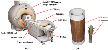
Figure 1. (a) Hyperion-IID scanner mounted on a patient table-top of a clinical 3 T MRI scanner thus creating a quick installable system. (b) Dedicated Tx/Rx MRI coil designed for the Hyperion-IID PET/MRI insert (shown separately).
Download figure:
Standard image High-resolution imageSince the 10 PET modules with their RF screens build an RF shielded environment in the inside, we decided to use a dedicated Tx/Rx MRI RF coil: a 12-leg-birdcage resonator (high pass version, tuned to the 1H frequency at 3 T, figure 1(b)) is used as an Tx/Rx coil for the MRI acquisition. The cylindrical mouse coil has a diameter of 46 mm and the sensitive area in axial direction covers approximately 12 cm yielding in combination with the PET system's field of view (FOV), which has an axial length of 10 cm, a combined cylindrical FOV with following dimensions: ∅ 46 mm × 100 mm. The resonator itself is surrounded by an RF screen that has a large distance of 7 cm to the resonator (air-filled to be PET transparent). Thus, the MRI RF coil is well isolated from its surrounding (including the PET detector) and is expected to provide a decent signal-to-noise ratio (SNR) performance.
The MRI system which was used to test the Hyperion-IID scanner is a Philips Achieva 3 T clinical MRI running software release 3.2.1.0. All system patches to add new functionality to the scanner were written and tested with this version. The MRI system is equipped with a Dual Quasar gradient system which employs two gradient amplifiers thus increasing the available slew rate of the system up to 200 T m−1 s−1.
3. Methods
3.1. Influence on MR performance
For data analysis and since all MRI data sets are typically shown scaled, all MRI data sets acquired and utilized in the following are rescaled to absolute values, so-called floating point values (FP values), enabling the comparison between scans. The only exceptions are MR images which are not further analyzed.
3.1.1. B0 field.
To evaluate the B0 field quality, volumetric B0 distortion maps for the entire FOV were acquired using a dual-echo FFE (fast field echo) sequence (TR/TE: 567/6.9 ms, TE extension ΔTE: 1 ms, Voxel size (VS): 1 × 1 × 1 mm3, volumetric scan) whereby the time difference between both echoes was ΔTE = 1 ms. A large water (clear water without additions) phantom filling the entire FOV served as signal source. The recorded phase images for each echo were unwrapped using an implemented 3D phase unwrapping algorithm. Per voxel the B0 deviation ΔB0 was calculated according to equation (1).

Here, Δϕ is the measured phase advance between the two echoes and γ is the gyro-magnetic ratio (42.576 MHz T−1) for protons. This experiment was performed without the PET scanner, which serves as reference scenario, and with the PET scanner to evaluate the influence of the PET system on the B0 field homogeneity. Since the MRI system is equipped with a dedicated shim system, we performed this experiment without any shimming (switched off in the preparation phases of the MRI scanner) and with an automatic volume shimming (higher-order shimming up to the 2nd order) implemented at the scanner. The size of the cuboid shim volume was set approximately to the size of the combined FOV (10 cm length in axial direction, 50 mm edge length).
In addition, we performed single voxel spectroscopy (SVS, free induction decay (FID) sampling without spatial encoding) for all four cases to study the line broadening effect of the B0 field inhomogeneity and to measure the altered field strength on absolute scale. The f0 determination preparation phase, responsible for the frequency locking typically necessary due to B0 field alterations, was switched off to keep the reference frequency of the synthesizer constant for all measured scenarios.
3.1.2. RF system.
Since the RF system is responsible for two tasks, spin excitation using RF pulses and signal acquisition, we performed two different characterization approaches: mapping of the B1 field strength in the FOV and evaluation of the noise level deterioration during signal acquisition (noise scans, SNR measurements).
B1 mapping. Since the presence of the PET scanner might influence the B1 distribution of the MRI RF coil and thus the distribution of the effective flip angle αe, we performed αe map measurements using a dual angle B1 mapping technique implemented at the MRI system (SE sequence, TE/TR: 10/600 ms, VS: 0.5 × 0.5 mm2, slice thickness: 0.5 mm, matrix: 300 × 300 (coronal, sagittal)/100 × 100 (transversal), FA: 90°, saturation delay: 250 ms). Since the scale of the flip angle (FA) distribution might fluctuate due to the power optimization preparation phase, which determines the peak power necessary to produce a 90° flip angle, and we are only interested in structural changes in the FA maps, all maps are normalized to the highest value. We used a 50 ml syringe filled with an CuSO4 phantom fluid (1000 ml demineralized water, 770 mg CuSO4.5H2O, 2000 mg NaCl, 0.05 ml H2SO4-0.1N solution) as homogeneous MRI phantom. The phantom was in fact rather large in comparison to a mouse phantom (20–30 ml) but still allowed a proper power optimization. Sagittal, coronal and transversal oriented B1 maps were acquired without and with PET detector installed in the system.
Noise scans. To study the impact on the MRI system's noise performance in detail, we performed dedicated noise scans (measurement protocol pre-installed at the MRI system): five consecutive TSE sequences (TSE sequence, TR/TE: 1044/256 ms, TSE factor: 32, acq. matrix: 1024 × 1024, bandwidth per pixel: 180 Hz) with shifted center frequencies (Δf0 = 0, ± 170 kHz, ± 340 kHz) are recorded and combined into one noise scan. For each bin along frequency encoding axis, the values along the phase encoding axis are histogrammed. Fits of Rayleigh distributions are performed for each bin to extract the intrinsic width of the 2D gaussian noise distribution. This width is then plotted as function of frequency yielding a noise scan with an overall bandwidth of about 1 MHz. This noise scan method was used to characterize the influence of the PET system by acquiring noise spectra without PET system and with PET system and for different optimization stages of the PET scanner: we have shown in Wehner et al (2014b) that the main noise source without optimization was the switched mode power supply unit (PSU) and that the optimization of the PSU's shielding led to a strong reduction of the induced noise during tests with single PET modules.
This optimization is in the present work extended to and evaluated with the fully populated scanner. In addition, we improved the power cabling of the scanner, meaning that all potential closed loops, created by pairs of power cables, are minimized especially in the proximity to the PSU's connection panel.
Typically, these noise scans are based on a standard imaging protocol and thus are performed with a very small flip angle (e.g. FA: 1° for the Philips Achieva system) leading to a major drawback of this method: to perform the test, no phantom causing an MRI signal after excitation is allowed to be inside the MRI system's FOV, thus the study of realistic PET/MR imaging (using e.g. FDG inside the FOV) scenarios is not possible. To overcome this limitation, a system patch was implemented which avoids the emission of RF pulses in general while keeping the remaining sequence structure untouched. In this way, noise scans using a FDG line source (starting activity A ≈ 21 MBq) were recorded to evaluate the impact of the PET system's workload on the noise performance.
Signal-To-Noise Ratio measurements. In addition to the noise scans, we performed SNR measurements using two different SE (Spin Echo) sequences (FA: 90°, TR/TE: 1000/50 ms, VS: 0.5 × 0.5 × 0.5 mm3, matrix size: 160 × 160) with different acquisition bandwidths: a scan with a small bandwidth (BW) (35 Hz/pixel, overall BW = 5.6 kHz) and a scan with a larger BW (220 Hz/pixel, overall BW = 35.2 kHz). We imaged a transversal slice of a cylindrical phantom filled with 20 ml (to ensure a proper load of the MRI coil) CuSO4 solution (same composition as described above) together with the above mentioned FDG line source which was attached to the phantom. In this way, SNR measurements were recorded as function of activity. The phantom itself was fixed in a dedicated phantom holder ensuring a proper and constant load of the MRI coil. The noise floor histograms of the different scans were taken according to NEMA Method 4 (NEMA 2008), namely in the outer regions in the image where no backfolding artifacts of the signal source occur. Fits of Rayleigh distributions to the noise floor histograms were performed for each scan to extract the quantitative level of the noise. The signal intensities were calculated by filling the signal carrying voxels in a histogram yielding a Gaussian distribution. After fitting, the mean value served as signal intensity measured in the specific scan.
3.1.3. Gradient system.
To investigate the influence on the gradient performance, we measured phase advances per voxel induced by additional eddy currents which, in turn, may be caused by the presence of the PET system. The technique is similar to correction methods used to improve echo planar imaging (EPI) sequence quality (Chen and Wyrwicz 1999). The basic idea is sketched in figure 2. The phase advances as function of time are, in a simplified model, determined by two main sources: (1) the B0 distortion causing a linear increase of phase as function of time (see figure 2 left, top) and (2) a constant phase advance caused by the modification of the gradient time course due to eddy currents induced in any conducting material (e.g. the PET scanner). By measuring phase maps for multiple echos, the odd echoes suffer from e.g. a positive phase advance whereas the even echoes suffer from an opposite one (see figure 2 left, middle and bottom). Both effects superimpose and lead to a time course indicated in figure 2 (right). Equation (2) describes the model:
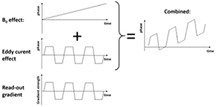
Figure 2. Sketch of the phase advance mapping technique: besides the temporary linear phase advance caused by a B0 distortion (left, top), eddy currents caused by fast switching gradients produce an alternating phase shift (left, middle) in a multi-echo readout (left, bottom). Both phase advance phenomena superimpose leading to a phase advance scheme shown on the right side.
Download figure:
Standard image High-resolution imageHere, Δf0 is the frequency shift caused by the B0 distortion, ϕEC is the height of the step function and thus quantifies the phase shift caused by the eddy currents, TE is the echo time of the first echo and ΔTE is the echo spacing between adjacent echoes.
To measure ϕEC caused by the switching gradients distortion, we recorded multiple phase images (10 echoes) using an FFE sequence (FFE sequence, TE/TR: 2.5/1311 ms (X and Z gradient) or 2.6/1319 ms (Y gradient), ΔTE: 3.2 ms, FA: 30°, VS: 2 × 2 mm2, slice thickness: 2 mm, matrix: 72 × 72, number of slices: 20, gradient strength: 4.5 mT m−1, slew rate: 26.5 T m−1 s−1). The same phantom as for the B0 scans was used. The plurality of phase images was unwrapped in 4D (in the three spatial and in the time dimension) to get an unwrapped time course of the measured phase per voxel. A fit of the model described above was performed per voxel to extract the phase advance ϕEC of the switching gradients. This parameter is then plotted per voxel yielding characteristic maps which contain the phase advances caused by eddy currents. Since the different gradient systems (X, Y and Z) might interact differently with the PET system (different magnetic fluxes due to geometric orientation), the sequence was modified in a way that, depending on the gradient switching direction under investigation, the read-out gradient trains were switching in X, Y or Z direction yielding ϕEC maps for all three gradient systems. These scans were performed without and with PET scanner to study the impact on the gradient performance due to the presence of the PET system.
To relate these findings to commonly used imaging sequences and to demonstrate the creation of ghosting artifacts, six 0.5 ml Eppendorf tubes, arranged along the Z axis of the MRI scanner with a pitch of 2 cm were imaged using EPI sequences with high EPI factor, extreme gradient strength and slew rates (FFE sequence, EPI factor: 17 (multi-shot acquisition), TE/TR: 32/66 ms, FA: 25°, VS: 0.25 × 0.25 mm2, slice thickness: 4 mm, coronal slice orientation, gradient strength: 30.9 mT m−1, slew rate: 198.2 T m−1 s−1). In contrast to the multi-echo FFE sequences used above, a small phase encoding gradient is inserted between the echo read-out. Thus, the phase shifts ϕEC lead to shifts in the acquired k space, in turn, yielding ghosting artifacts (multiple ghosts are expected since the EPI images are recorded in multi-shot mode (Hennel 1997)). As for the multi-echo acquisition, the direction of the EPI read-out gradient was changed accordingly.
3.2. Influence on PET performance
All PET data acquired to analyze the influence of the MR operation on the PET performance are acquired in raw mode, meaning that the raw detector data is dumped to disk. The sensor tiles are in all following cases operated with an overvoltage (OV) of 2.5 V, trigger scheme 3, a validation scheme of 4-OR, a validation length of 40 ns and an integration length of 165 ns. Using these settings, a dSiPM pixel requires on statistical average 3.0 ± 1.4 microcell (also called SPAD (Single Photon Avalanche Diode)) breakdowns (assuming an uniform photon distribution) to generate a trigger signal which starts a validation phase of programmable length (validation length). At the end of this validation phase, a validation threshold has to be passed to accept the trigger event. Assuming an uniform photon distribution, the aforesaid validation scheme of 4-OR requires on average 17 ± 6.2 fired microcells. If the event is accepted, the event is read out at the end of an integration phase of programmable length (integration length). Details about the working principle and the different trigger schemes and possible validation schemes can be found in Frach et al (2009) and Tabacchini et al (2014).
The cooling chiller was set to 5 °C, which leads to tile temperature on average of around 12 °C, and we configured each sensor tile with inhibit maps with 20% deactivated cells. We have chosen these parameters as they were repeatedly used and thus can be considered as a stable, conservative operating point. The PET raw data was clustered in to single events and an Anger algorithm was used for crystal identification. An energy calibration was applied on crystal level. The following quality criteria are applied to select single events:
- Neighbor criteria: all neighboring sensor dies have to be triggered
- Minimum number of photons: 400
- Maximum number of photons: 2600
- Energy window: (411–561) keV
After selection, flood map histograms are generated for each sensor stack and the energy resolution is calculated per stack for the entire scanner whereby all quality criteria are applied except for the energy window yielding a complete energy histogram. After performing a coincidence search, coincident events were used to perform a time delay calibration on sensor die level and later on utilized to determine the system's coincidence resolution time (CRT) (Schug et al 2014).
3.2.1. B0 field.
The influence of the B0 field on the PET scanner was studied by monitoring the scanner's environmental sensors (temperature, voltage and current monitors) and acquiring PET raw data to compare flood map histograms for two scenarios: (1) the scanner outside the B0 field and (2) inside the B0 field. All acquired data for both scenarios were compared and analyzed to search for influences.
3.2.2. RF system.
To test for sensitivity of the PET system's electronics for RF pulses, we applied extensive demanding TSE sequences (TSE factor: 16, TE/TR: 21/333 ms, peak B1 amplitude: 30 µT, matrix: 160 × 128, VS: 2.5 × 2.63 mm2, slice thickness: 20 mm, BW: 442.8 Hz px−1) while acquiring PET raw data. This test sequence was applied in a time window of about 30 s while the rest of the PET data acquisition was unharmed by the MR operation and thus served as reference scan. Energy and CRT resolution were determined accordingly to the description above and are compared for the two scenarios without and with MR operation.
3.2.3. Gradient system.
Gradient stress tests.
As shown in Wehner et al (2014b), the PET detector shows sensitivity to gradient switching, especially when the Z gradients are operated. To study this phenomena in detail and to investigate the scalability of the observed degradation effects, we have implemented a dedicated test sequence, sketched in figure 3, which allows the precise definition of gradient parameters such as the gradient strength (GS), slew rate (SR), switching direction, switching duty cycle (SDC). We used this sequence to test the influence on the PET performance using various gradient parameter sets: for three different gradient strengths (10, 20, 30 mT m−1), parameter scans with variable SR and SDC were performed. The gradient amplifiers were in all cases operated in high SR mode to increase the available SR to 200 T m−1 s−1. The maximum gradient strength was set to 30 mT m−1 in the system configuration for security reasons. As gradient switching direction, we chose the Z gradient since most degradation is expected from this gradient system as already described earlier (Wehner et al 2014b). The applied parameter sets are summarized in table 1. The different test sequences were applied in time windows of about 20 s while taking PET raw data. After raw data processing, the energy and CRT resolution, as typical performance parameters of the PET system, were calculated for each scenario and compared to reference scans performed without any gradient activity.
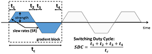
Figure 3. Sketch of the newly implemented gradient test sequence: it gives complete control over the gradient system meaning that strength, slew rate, switching direction as well as asymmetries or duty cycle can be adjusted accurately.
Download figure:
Standard image High-resolution imageTable 1. Overview of the parameter ranges of the gradient test sequences which were applied while taking PET raw data. The gradients were switching in all test scenarios in z direction.
| Parameter | Range |
|---|---|
| Direction | z |
| Strength (mT m−1) | 10, 20, 30 |
| Slew rate (T m−1 s−1) | 25, 50, 100, 150, 200 |
| Switching duty cycle (%) | 20, 40, 60, 80,100 |
Imaging protocols.
To relate the findings from the dedicated test sequence to real-life imaging scenarios, we performed typical MR imaging sequences such as T1 and T2 weighted TSE (Turbo Spin Echo) sequences, T1 and T2 weighted FFE sequences and EPI sequences. The parameters for the imaging examples are motivated by clinical predefined MR image acquisition protocols which were pre-installed on the MRI scanner. These clinical MRI sequences were adapted for our small animal coil, meaning that most notably the voxel size, slice thickness and acquisition matrices were changed. Supplementary table S1 (stacks.iop.org/PMB/60/062231/mmedia) summarizes the most important sequence parameters. All imaging sequences were applied while following the same procedure as described above, namely taking PET raw data and processing it accordingly. The resulting performance parameters are then compared to a reference scan without MRI activity.
4. Results
4.1. Influence on MR performance
4.1.1. B0 field.
The results of the B0 field characterization are shown in figure 4: representative slices in sagittal slice orientation from the center of the FOV are shown for all four scenarios (top row: before shimming, bottom row: after shimming, left: without PET system, middle: with PET system). A comparison of profile lines in axial direction from the center of the FOV without (black) and with (red) PET system is shown on the top right before shim optimization and at the bottom right after the application of shimming. Without shimming, the presence of the PET scanner clearly changes the distortion profile in axial direction from a linear distortion profile to a 2nd order profile. The VRMS (volume RMS) values (without PET system: 0.34 ppm, with PET system: 0.28 ppm) as well as the peak-to-peak values (without and with PET system: 1.2 ppm) are in both cases on a similar level. After the shim optimization, the linear distortion profile of the scenario without PET detector is almost corrected as shown by the profile line: we measure a peak-to-peak value of about 0.28 ppm and a VRMS value of 0.03 ppm. For the scenario with PET system, the higher order shim of the MRI system was able to correct the 2nd order profile strongly. Here, the VRMS and peak-to-peak values are reduced down to 0.08 ppm and 0.71 ppm, respectively. Figure 5 shows the results of the SVS (left: before shimming, right: after shimming, black: without PET system, red: with PET system). Without the application of shimming, we measure a lowering of about 1.5 ppm (200 Hz) on absolute scale when the PET system is inserted into the MRI. The spectra show a clear line broadening/peak splitting caused by the unoptimized field distribution, whereas after shimming, the spectrum without PET insert shows an unsplitted Lorentz peak as expected from a single water line. With PET system present, the spectra is clearly improved after shimming, but still shows a residual off-center component caused by remaining higher-order components (see the corresponding profile line in figure 4 (bottom, right, red)).

Figure 4. Results of the B0 characterization: example slices in sagittal slice orientation are shown for the scenarios without (left) and with (middle) PET system before (top row) and after shimming (bottom row). Characteristic profile lines from the center of the FOV along the Z axis are shown on the right (black: without PET, red: with PET).
Download figure:
Standard image High-resolution image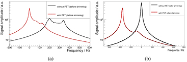
Figure 5. Results of the single voxel spectroscopy measurements are shown before shimming (a) and after the application of shimming (b). The 'without PET' scenario is shown in black, the one with PET system in red.
Download figure:
Standard image High-resolution image4.1.2. RF system.
B1 scans.
Figure 6 shows the results of the B1 scans: the normalized flip angle distribution (color coded) is shown for the sagittal slice orientation in the top row, the coronal orientation in the middle row and the scans in transversal orientation in the bottom row. The measurements without PET detector are shown on the left, the ones with PET system in the middle and a difference map is shown on the right. We measure no critical structural change in the flip angle distribution. Only minor changes in the sagittal and coronal orientations in the range of ± 5% are visible. These changes are located in the marginal regions (in axial direction) of the sensitivity profile. The transversal slice was acquired in the axial center of the FOV and, in agreement with the sagittal and coronal scans, no considerable changes are observed for this orientation.
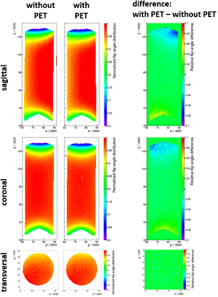
Figure 6. Results of the B1 map measurements (sagittal: top, coronal: middle, transversal: bottom): the normalized flip angle distribution is shown color coded for the scenario without (left) and with (middle) PET system. A difference map is shown on the right (note the difference in the color scale).
Download figure:
Standard image High-resolution imageNoise scans.
Noise scan results of the different optimization steps are shown in figure 7: a reference scan is shown in black, a scan using the unoptimized, single-ring equipped prototype scanner (equipped with 20 of 60 possible detector stacks, as presented in Wehner et al (2014b)) is shown in red for comparison reasons. All further measurements were performed with the fully populated PET scanner (see section 2). A measurement with optimized PSU shielding as described in Wehner et al (2014b) is shown in cyan and the final result of the optimization (including a optimized power cabling of the PET scanner) is shown in green. As clearly visible, we were able to suppress the noise floor degradation from initial 70–320% down to 2–15% by applying all optimizations. Without improving the cabling of the PET scanner, the noise level degradation is still clearly improved (30–210%), but still considerably higher than the fully optimized version. All scans with active PET system feature peaks which are high harmonics of the PSU's switching frequency (≈250 kHz) meaning that even after optimizing the PET system, the PSU remains the main noise source (Wehner et al 2014b).
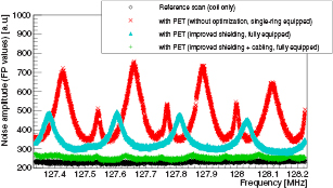
Figure 7. Noise scan results: a reference measurement is shown in black, a measurement using the unoptimized version of the PET system is shown in red. After optimization of PSU's shielding, the cyan colored curve was obtained and the results after the full optimization is shown in green.
Download figure:
Standard image High-resolution imageFigure 8 summarizes noise scans of the optimized PET system with different activities inside the PET scanner: a reference scan is shown again in black, a scan with the PET system switched on but without activity is shown in green and two example scans with different activities A are shown in orange (A ≈ 7.6 MBq) and red (A ≈ 20.2 MBq.). Despite the presence of the 250 kHz harmonics already described above, it is to note that the peak height is not changing for the different 'with PET' scenarios, but the peak position is. The peak position is shifting because of the changing load of the switched-mode PSU. Consequently, the noise level degradation expected during a simultaneous PET/MRI experiment is depending of the peak position. Overall, the noise level degradation (NLD) is expected to range in all scenarios between 2% and 15% . No narrow peaks indicating digital noise artifacts are observed in any scans meaning that no zipper artifacts are expected in imaging experiments.
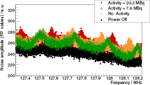
Figure 8. Noise scan results for different activities: a reference scan is shown in black, a scan with the PET system switched on but without any activity is shown in green. Two example measurements with activity are shown in orange (7.6 MBq) and red (20.2 MBq).
Download figure:
Standard image High-resolution imageSNR study.
Results of the SNR study are shown in figure 9(a): the signal intensities (top row), the noise levels (middle row) and the measured SNR values (bottom row) are shown for the SNR scans with small BW (left) and larger BW (right) as function of activity A. The signal intensities are for all measurements on a stable level (within 5%). However, we observe a slight decreasing trend for higher activities (towards the beginning of the measurements series) which could be related to a temperature change over time of the MRI phantom itself or the RF-coil affecting the contrast of the images acquired. For the noise level, we observe a clear worsening, when the PET insert is switched on (the scan without PET insert is shown at A = − 1 MBq). The same holds true for the SNR measurement. Overall both SNR imaging sequences (small and large BW) show the same behavior. The NLD, defined as the ratio between the noise level measured with PET and the one measured without PET (shown at A = − 1 MBq), is drawn as function of activity in figure 9(b) (blue: SNR measurement with small BW, red: SNR measurement with large BW, green: calculated from noise scans): In agreement to the noise scans shown above, the NLD measurements stay for all activities between 2–15% . The modulation observed in this study is related to the position of the 250 kHz harmonics with respect to the sensitive frequency bandwidth of the SNR imaging protocol as the NLD measurements calculated from the noise scans (green) show. More importantly, no strong dependence of the NLD is observed as function of activity.
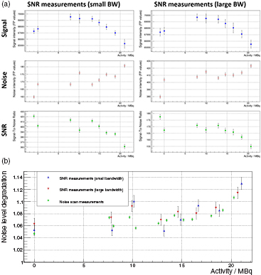
Figure 9. Signal (top), noise (middle) and SNR (bottom) measurements as function of activity for the SNR measurement sequences (left: small BW, right: large BW) are shown in (a). Noise level degradation as function of activity are shown in (b) (blue: small BW SNR scans, red: large BW SNR scans, green: noise scans).
Download figure:
Standard image High-resolution image4.1.3. Gradient system.
Figure 10(a) shows the results of the gradient performance study: the ϕEC maps are shown for all three gradient systems (left: X, middle: Y, right: Z) without (top row) and with (bottom row) PET system present. A profile line comparison for the Z gradient from the center of the FOV in axial direction is shown in figure 10(b) (black: without PET system, red: with PET system). While almost no eddy current disturbance is visible in the measurement without PET system for all three switching directions, a significant phase advance is observed when the PET system is present and the Z gradient is used as read-out gradient.
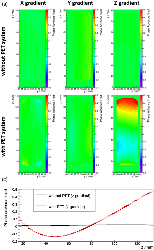
Figure 10. Results of the ϕEC mapping: ϕEC maps without (top row) and with (bottom row) PET insert are shown in (a) for all different read-out directions (left: X, middle: Y, right: Z). Characteristic profile lines (for Z read-out gradient) are shown in (b) and demonstrate the impact of the PET electronics on the gradient performance.
Download figure:
Standard image High-resolution imageThe results of the EPI scans are shown in supplementary figure S2 (stacks.iop.org/PMB/60/062231/mmedia) and support the observations made above: when using the Y gradient as read-out gradient, no difference between both scenarios are observed. None of the two images show severe ghosting artifacts leading to a signal drop in the signal volume. However, when using the Z gradient as read-out gradient (in agreement to the results of the gradient performance study), the image acquired with PET insert shows ghosting artifacts whereas the one without PET insert does not.
4.2. Influence on PET performance
While the PET system shows a clear influence on all the three sub-systems of the MRI system, only the operation of the MRI machine's gradient system reveals a sensitivity of the PET electronics to gradient switching. For the other sub-systems (B0 field and RF system) only minor influences which do not impact the PET performance are observed.
4.2.1. B0 field.
Figure 11 shows representative, normalized flood map histograms of a single (out of 60) sensor stack measured outside the B0 field (left) and inside the B0 field (middle). A difference map of both flood map histograms is shown on the right. No structural differences such as flood map distortions and thus no influences on the flood map quality due to B0 field are observed. The same holds true for all other 59 detector stacks. Supplementary figure S3 (stacks.iop.org/PMB/60/062231/mmedia) shows the corresponding energy spectra after energy calibration on crystal bin level for the entire sensor stack (sum of the energy spectra of all crystal bins) measured outside (blue) and inside (red) the B0 field. We measure for both scenarios an energy resolution of about 12.4% . No significant difference between both measurements is observed.
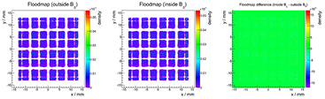
Figure 11. Normalized flood map histograms for Anger positioned singles events measured outside the B0 field (left) and inside the B0 field (right). A difference map (inside B0–outside B0) is shown on the right.
Download figure:
Standard image High-resolution imageWe only observed some minor impacts on the PET system while being operated inside the B0 field:
- Small shifts of the bias voltage of about 0.05 V.
- Systematic shifts of the temperature measurement to lower values of about 0.3 °C.
4.2.2. RF system.
We did not observe any PET performance degradation caused by the emission of RF pulses. Both the singles and coincidences count rate as well as performance parameters such as the energy and timing resolution are unaffected. Temperature, voltage and current measurement did not show any abnormalities like heating effects or ripples on the supply voltages. An example measurement while applying the RF stress test is given in supplementary figure S4 (stacks.iop.org/PMB/60/062231/mmedia).
4.2.3. Gradient system.
As stated above and shown in Wehner et al (2014b), the application of highly demanding stress tests revealed a sensitivity of the PET electronics to switching gradients. This sensitivity manifests itself in a degradation of the energy and timing resolution. The energy resolution degradation is related to a ripple in the bias voltage induced by switching gradients and amplified by the low-dropout voltage regulators (Wehner et al 2014a, 2014b).
Figure 12 shows the maximum degradation ((a): energy resolution, (b): timing resolution) observed for the scanner (single stack, green: without gradient activity, red: with switching gradients): these measurements were acquired with a GS of 30 mT m−1, a maximum SR of 200 T m−1 s−1 and a SDC of 100% (for the energy resolution degradation) (80% for the CRT degradation). Thus, the gradient waveform is triangular (for the CRT degradation almost triangular) and at the limit of what the gradient amplifiers are able to supply. For the energy resolution, we measure a relative degradation of approx. 10.4% (without Z gradient: Eres ≈ 12.87%, with Z gradient: Eres ≈ 14.2%). For the timing resolution, we measure without Z gradient a FWHM of about 555 ps and with Z gradient a worsening of the FWHM to 635 ps (degradation: 14.4%).
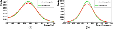
Figure 12. Worst case scenarios with maximum possible slew rate (200 T m−1 s−1) and switching duty cycle of 100% (left) or 80% (right): The application of the test sequences lead to a degradation of the energy resolution ((a), green: without switching z gradients, red: with switching z gradients) of up to 10.4% and timing resolution ((b), green: without switching z gradients, red: with switching z gradients) of up to 14.4%.
Download figure:
Standard image High-resolution imageFigure 13(a) shows the angular dependence of the energy resolution degradation (ERD). The ERD of each sensor stack (in percentage points) is plotted as function of the ring position (as indicated in figure 13(b)). This measurement was acquired using the maximum demanding Z gradient test sequence (GS: 30 mT m−1, SR: 200 T m−1 s−1, SDC: 100%). We observed a mirror symmetry to 180° and that the stacks at the bottom of the PET ring (around 180°) show less degradation than the modules at the top. This is caused by a shift of the PET iso-center with respect to the MRI iso-center (the PET iso-center is approx. 4.5 cm higher than the MR iso-center). Thus, the modules at the top are closer to the gradient coils and see a higher magnetic flux. Consequently, they are more prone to any induction related degradation effects.
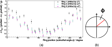
Figure 13. Energy resolution degradation (ERD) for each sensor stack as function of the ring position (as depicted in (b)) in shown in (a). For reasons of clarity, the stack positions of the first (third) ring shifted by +(−)2°. We observe a mirror symmetry of the scanner and that the modules on the top of the ring (modules with ϕ of about 0° or 360°) show more degradation than the modules at the bottom of the ring.
Download figure:
Standard image High-resolution imageTo investigate the scalability of these findings, we studied the performance degradation as function of the different gradient parameters. For the ERD, we measured a graph as shown in figure 13 for each parameter set (GS, SR, SDC). Since the modules on the top of the ring are most sensitive, we averaged the ERD levels of the top four modules (20 detector stacks in total) and used the resulting value as measure for the maximum observed degradation strength (Max. ERD). Since the impact on the entire system is also of relevance, we calculated the average ERD on system level including all modules (Avg. ERD). The CRTD (CRT degradation) was calculated on system level, meaning that all PET modules were considered in the calculation, since the highly affected modules at the top are counterbalanced by opposing less effected modules. A separate treatment for the modules at the top as we did for the ERD measurement is not possible because the CRT is measured in coincidence mode.
Figure 14 depicts the results of the gradient parameter scans: for three gradient strengths (left: 10 mT m−1, middle: 20 mT m−1, right: 30 mT m−1), the avg. ERD (top row), the max. ERD (middle row) as well as the CRTD (bottom row) are shown. The maximum degradation level for the avg. ERD is about 5.8%, for the max. ERD 8.8% and for the CRTD 14.3% . For a given gradient strength, we observe that the SDC (determines the statistical weight of PET data acquired during gradient switching) and SR (determines dB/dt) have a severe control over strength of the degradation effects (examples for a GS of 20 mT m−1 are given in supplementary figure S5 (stacks.iop.org/PMB/60/062231/mmedia)). In addition, a saturation effect for increasing SDC at high SR becomes apparent. This saturation effect seems to intensify for lower gradient strength leading to a shift of the peak degradation level to lower SDCs. Impacts on singles or coincidences count rates as described in Wehner et al (2014b) are observed if provoked by applying narrow energy cuts (see supplementary figure S6 (stacks.iop.org/PMB/60/062231/mmedia) for a measurement with maximum SDC (100%) and SR ranging from 25 T m−1 s−1 up to 200 T m−1 s−1). Without this provocation (by e.g. using a wider energy window), no losses of events were observed. Since the switching gradients obviously couple to the PET detector's hardware leading to eddy current dissipated, we monitored temperature sensors on the PET modules: although we observed temperature changes on SPU level (temperature measurements are shown in supplementary figure S7 (stacks.iop.org/PMB/60/062231/mmedia)), the temperatures measured on the sensor tile were stable and did not show any heating effects.
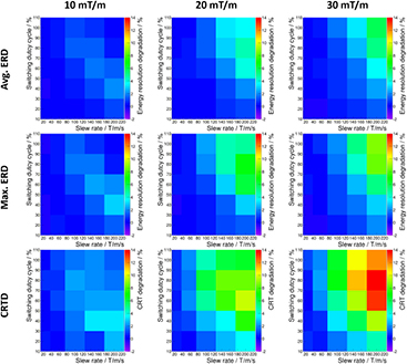
Figure 14. Energy (top: average. ERD, middle: max. ERD) and timing (bottom) resolution degradation for three different gradient strengths (left: 10 mT m−1, middle: 20 mT m−1, right: 30 mT m−1). For each gradient strength, the relative degradation is measured as function the SDC and the SR.
Download figure:
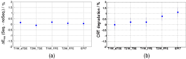
Standard image High-resolution imageFigure 15 shows the results of the imaging sequence test: in agreement to the parameters tests presented above and due to the comparatively small SDC of ⩽20%, we did not observe any severe degradation effects. Only for the EPI and T2W-FFE sequences which also provide the highest SR and SDC of all test sequences, we observe in the CRT degradation a hardly measurable impact.
Figure 15. Enery (evaluated for the upper modules, max. ERD) (a) and timing (b) resolution degradation for imaging test sequences: only for the EPI sequence, a measurable degradation effect was observed.
Download figure:
Standard image High-resolution image
5. Discussion
5.1. The B0 field
On the MRI side, the B0 field distribution is substantially altered when the PET system is inserted into the MRI system: without shim optimization, the PET system with its mainly positive susceptibility distribution lowers the B0 field strength in the combined PET/MRI FOV resulting in a 2nd order distortion. In comparison to the linear distortion profile caused by the unoptimized shim for the scenario without PET system, this 2nd order distortion is expected to impose stronger requirements on the MRI scanner's shimming system meaning that a higher order shimming system is required. After the application of shimming, especially the field homogeneity measured with the RF-coil only is strongly improved: with a VRMS value of about 0.03 ppm (4 Hz) and a peak-to-peak value of about 0.28 ppm, the RF-coil itself provides an MRI environment likely good enough to enable also the application of more advanced MR imaging (with e.g. spectral selective prepulses) or spectroscopic protocols. With the PET system installed and after applying an automatic higher order shim, we obtain a clearly improved field homogeneity in comparison to the measurement before shimming. The VRMS value of about 0.08 ppm, the peak-to-peak value of 0.71 ppm as well as the axial distortion profile are clearly better than before shim optimization showing that the MRI scanner's shim system is able to compensate most of the distortion. However in comparison to the 'coil-only' scenario, the field quality with PET system is noticeably worse (we measure approximately a factor of 2.5 worse VRMS and peak-to-peak values) and the axial distortion profile reveals remaining higher order components. Nevertheless, we consider the field quality as probably good enough for many (also challenging) MR acquisition protocols especially for morphological MRI scans. Negative impacts on specific protocols need to be evaluated for the given situation. It is to note that this investigation profits from the usage of a small animal coil with a diameter of 46 mm. Using a coil with a larger diameter (e.g. designed for rabbits) would increase the available FOV. As a consequence, the outer regions in radial direction of this increased FOV would be closer to the PET modules. Thus a localized distortion induced by the PET modules might have a more severe influence on the field quality and could reveal stronger higher order components which are not recoverable by the MRI's shim system. The application of local shimming (active or passive) on PET detector level, as described in Wehner et al (2014a), might help to overcome this potential issue.
On the PET side, only minor influences are observed. When the PET system is inside the B0 field, the measured temperature shifts can be regarded as mismeasurements. The temperature sensors show a clear B0 dependence. These kind of mismeasurements are of limited relevance, especially because the PET system is operated inside a constant B0 field, hence we are dealing with a constant mismeasurement which is easily correctable. More relevant is the observed shift of the applied bias voltage caused by a magnetic field sensitivity of the voltage regulators. However, the shifts of about 50 mV are smaller than the step size of the used digital-to-analogue converters, thus are almost negligible and hardly correctable. A corresponding mismatch in the energy calibration is easily corrected by a recalibration for the 'inside B0 field' scenario.
5.2. The RF system
On the MRI side, the B1 map measurements suggest only minor differences when the PET system is present. Additionally, these alterations are only visible in the marginal regions of the sensitivity profile of the MRI coil. Hence, no substantial impact on the overall imaging performance of the MRI coil is expected especially because the sensitivity of the MRI coil is dropping in this region anyhow and thus is not the preferred region to choose when performing imaging experiments. The induction of noise originating from the PET scanner is on an acceptable level. The SNR degradation of about 2–15% can easily be covered by e.g. increasing the MRI scan time by only up to ∼4–30% . This result was achieved after optimizing the PET system, namely the PET system's PSU as described in Wehner et al (2014b) and the power cabling. More importantly, the noise scans did show only a broadband modulation, but no digital noise peaks, meaning that no zipper artifacts are observed and expected in imaging experiments. This is in particular notable since the entire PET scanner is based on digital technology and is operated inside the MRI system's FOV. However, things might change when the PET scanner is used in combination with another RF-coil (e.g. an RF-coil with a larger diameter designed for larger animals): the utilized Tx/Rx mouse coil is isolated quite well from its surrounding due to the large distance of the RF screen to the resonator. As a consequence, the NLD optimization might have been easier compared to scenarios with other coils which might interact much more with their surrounding. Besides a potential increased SNR loss, the higher proximity of the PET modules to a larger RF resonator might result in a stronger alteration of the B1 field (and thus flip angle) distribution.
On the PET side, we did not observe any performance degradation caused by the emission of RF pulses. Three main reasons support this observation: First, the peak power used by the MRI system to produce the target B1 field strength of 30 µT is in the range of only a few Watts (4–10 W, depending on the load of the RF-coil). Especially in comparison to other MRI coils such as a Tx/Rx head coil (peak power in the order of 500–1000 W), the peak power is rather small. Second, the MRI resonator is isolated quite well from its surrounding, meaning that the current distribution on the RF screen is expected to be comparatively small. Consequently, the B1 distribution in the outer region, where an interaction with PET modules might occur, is expected to be negligible. Finally, the PET modules themselves are enclosed by a carbon fiber housing which additionally protects the PET electronics from any RF pulses. This reasoning is of course only valid for scenarios where a well isolated RF-coil is used. As stated above, things might change when different RF-coils are used such as RF-coils designed for larger animals. As a consequence, larger peak powers would be needed to produce the desired B1 field strength and the strength of the B1 fields in the outer region (beyond the RF screen of the resonator) would intensify. This might result in more severe consequences for the PET electronics leading to a potential performance degradation. However, no interference investigations with a different RF coil were performed (e.g. a coil with a larger diameter).
5.3. The gradient system
On the MRI side, eddy-current-induced phase advance measurements showed that the PET insert introduces additional disturbances to the gradient switching: while the distortions are relatively small for the X and Y gradient system, a clear profile change is observed for the Z gradient system. This is not surprising since we observe also for the switching Z gradients the strongest degradation of the PET system's performance (Wehner et al 2014b). However, when performing EPI sequences to evaluate the impact on real imaging scenarios, the differences between the 'with PET' and 'without PET' scenarios are almost negligible especially when the X and Y gradients are used as read-out gradients. Only for high EPI factors in combination with a read-out gradient in Z direction, differences between the measurements without and with PET system appear. Hence, for e.g. diffusion-weighted imaging or fMRI, where intense and fast EPI acquisitions are used, we might face some limitations when the PET system is installed.
On the PET side, we observed a degradation of the energy (up to 10%) and timing (up to 14%) resolution when the gradient system is switching. We see the most severe degradation in combination with the switching Z gradient (Wehner et al 2014b), the maximum SR available at the MRI system (200 T m−1 s−1) and very high SDC (80–100%). All three gradient parameters (GS, SDC and SR) had a strong influence on the degradation observed. Interestingly, we observed a saturation effect which led to a shift of the measured peak degradation level to smaller SDC while being always observed for the highest SR. This saturation effect is likely caused by a smoothing effect on the gradient edges (Lenz's law), which becomes more prominent for higher SRs and higher SDCs, thus lowering the overall dB/dt for a gradient cycle. The effects intensifies for lower GS presumably explainable by the higher switching frequency of the gradients for the lower GS (the switching frequency is increased because the SDC and SR are kept constant). This increased frequency in combination with the smoothing effect also leads to a reduced overall dB/dt (for a larger time window) thus lowering the degradation level. Despite this saturation effect, the degradation level shows a linear behavior as function of the SR, which determines dB/dt and thus controls the strength of the induction process, and SDC, controlling the statistical weight of PET data acquired during a rising or falling gradient slope. More importantly, we observe in regions with small SR (SDC) and arbitrary SDC (SR) hardly measurable degradation effects. In agreement with this observation and since the SDC of normal imaging protocols is expected to be rather small (for the presented set of sequences ⩽20%), we observed barely measurable influences. Nevertheless, the set of imaging protocols we presented covers of course only a small part of all potential useful MRI acquisition protocols. One can define more demanding sequences (e.g. fast EPI sequences used in functional MRI) with higher 'slew rate/duty cycle' combination which would lead to a more dramatic influence. However, we already presented the maximum degradation level observed for our PET configuration and these degradation levels are still acceptable in a preclinical environment: On the one hand, the energy resolution degradation with up to 10% is covered by a wide energy window (in the range of (265–650) keV) used to select interesting events for image reconstruction. Hence, no relevant event rate drops caused by the application of the energy filter are expected and more importantly, we did not see losses of events (without the application of the energy filter) caused by the switching gradients. On the other hand, the timing resolution is currently, and especially for the presented PET system, in a preclinical environment not of great relevance since the combined FOV of our PET/MRI scanner has a diameter of about 46 mm and is thus too small to dramatically benefit from TOF-PET. However, things might be different when the same PET architecture is used at different geometries. As the observation in figure 13 showed, the degradation levels scales drastically with the proximity to the gradient coils where the magnetic flux of the gradient fields intensifies. In addition, the results presented are performed with the trigger setting 3, which is working well for PET image acquisition but is also known not to provide the best timing performance. Using the first photon trigger, the CRT of our system is substantially better (CRT ∼ 250 ps) (Schug et al 2014). Consequently, the strength of degradation effect observed might become more prominent. Thus, a PET scanner with modules closer to the gradient coils which is operated at lower trigger setting (e.g. in a more clinical environment) might face much higher degradation effects. To solve this issue, the PET detector's hardware needs to be improved. Investigations regarding the origin of the CRT degradation and the bias voltage ripple causing the energy resolution degradation are currently on-going.
6. Conclusion
Since MRI measurement protocols in their diversity impose a wide range of different requirements regarding MR-compatibility, a comprehensive study including scalability tests on interference phenomena between the PET detector and all of the MRI scanner's subsystems and vice versa is mandatory to reliably assess the MR-compatibilty of such a hybrid device. We have presented such an MR-compatibility study of a preclinical, digital PET/MRI insert which is designed to be operated inside a 3 T clinical MRI system. In contrast to other PET/MRI systems, the entire PET detector's electronics are installed and operated inside the MRI system's FOV. Overall the level of performance degradation on both imaging systems is on an acceptable level meaning that a simultaneous image acquisition is possible. However, we see a clear influence on the MRI environment when the PET system is installed: the B0 field is substantially distorted with the PET system installed. This induced distortion profile is dominated by lower orders, thus allowing the application of higher order shimming to recover most of the field homogeneity (VRMS value = 0.08 ppm, peak-to-peak value = 0.71 ppm). With respect to the RF and gradient system, we observe a noise level degradation of 2–15% and an occurrence of phase advances caused by induced eddy currents in the PET system's hardware components (mainly with switching Z gradients). These effects might have a limiting influence on the MRI performance when advanced MR protocols are applied which impose high requirements on the MRI environment. Examples for such protocols are fMRI studies which make extensive use of EPI sequences (limitations due to eddy currents) or MRI scans with highly selective prepulses depending on a high B0 field homogeneity (e.g. CEST, Bright Iron sequences). On the PET side, we almost exclusively see a sensitivity of the PET electronics to gradient switching which manifest itself in a degradation of energy (up to 10% degradation) and timing (up to 14% degradation) resolution. This level of degradation can still be considered acceptable since the timing resolution is not critical in a preclinical environment and the energy resolution degradation has no influence on the PET performance if larger energy windows as typically used in preclinical imaging are applied.
Acknowledgments
The presented work is financially supported by Philips Research Europe, Aachen, and is part of the ForSaTum project (NRWEU Ziel 2- Programm 2007 -2013) and MEC (Wellcome Trust 088641/Z/09/Z).