


Abstract
In this paper, we study a high-order finite element approach to simulate an ultrahigh finesse Fabry–Pérot superconducting open resonator for cavity quantum electrodynamics. Because of its high quality factor, finding a numerically converged value of the damping time requires an extremely high spatial resolution. Therefore, the use of high-order simulation techniques appears appropriate. This paper considers idealized mirrors (no surface roughness and perfect geometry, just to cite a few hypotheses), and shows that under these assumptions, a damping time much higher than what is available in experimental measurements could be achieved. In addition, this work shows that both high-order discretizations of the governing equations and high-order representations of the curved geometry are mandatory for the computation of the damping time of such cavities.
Export citation and abstract BibTeX RIS

Original content from this work may be used under the terms of the Creative Commons Attribution 3.0 licence. Any further distribution of this work must maintain attribution to the author(s) and the title of the work, journal citation and DOI.
1. Introduction
In 2012, Serge Haroche and David Jeffrey Wineland were jointly awarded the Nobel prize in physics for ground-breaking experimental methods that enable measuring and manipulation of individual quantum systems [1]. Basically, they succeeded in building devices where quantum particles (such as photons or ions) can be trapped [2]. A few years before, in 2007, Serge Haroche and his coworkers were able to record the birth and death of a photon in a cavity [3, 4], by using an ultrahigh finesse Fabry–Pérot superconducting resonator [5]. This open cavity consists of two superconducting (niobium at 0.8 K) toroidal mirrors (see figure 1) with an extremely high manufacturing precision, as shown on the geometrical parameters of table 1.
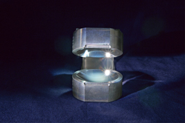
Figure 1. Picture of the two mirrors developed in [5] (used with the kind permission of Michel Brune, Laboratoire Kastler Brossel, Paris, France).
Download figure:
Standard image High-resolution imageTable 1.
Geometry of the mirrors in  .
.
| Diameter | Radius of curvature | Maximum deviation | Distance between apexes |
|---|---|---|---|
| 50 | 40.6 (major) | 3 × 10⁻⁴ (peak-to-valley) | 27.57 |
| 39.4 (minor) |
The cavity is resonant at  with a measured damping time of approximately
  . Simply put, this high damping time means that, if a photon appears inside the cavity, it will somehow bounce back and forth for a very long time without interfering with the outside world. By taking advantage of the extremely long lifetime of the photon inside the cavity, Serge Haroche and his coworkers were then able to record the birth, life and death of a photon.
In 2014, attempts were made to model the photon cavity, by using the classical time-harmonic Maxwell equations with the finite element (FE) method and a quasimodal analysis [6]. In particular, by analyzing the eigenmodes of the cavity, the resonance frequency as well as the damping time can be recovered. In their paper, the authors were able to compute the resonance frequency of the cavity, but did not reach a numerically converged value for the damping time with respect to the FE mesh density. The purpose of this paper is to compute the damping time of the photon cavity by using a high-order FE method. In addition, by studying an idealized setup, the performance limits of the cavity are assessed. To the best of our knowledge, the following analysis with high-order techniques is performed for the first time.
This paper is organized as follow. First, in section 2, it is explained how classical electromagnetic numerical computations, exploiting the FE method and a perfectly matched layer (PML), can be used to estimate the lifetime of a photon in an open cavity. Furthermore, the use of a high-order FE approach is motivated. Then, in section 3, the numerical setup is presented. The paper continues with some numerical results in section 4. Section 5 discusses the computational bottleneck introduced by the memory scaling. In order to push further our analysis of the cavity, a two-dimensional setup presenting the same limitations regarding the lifetime is studied in section 6. Finally, conclusions are formulated in section 7.
2. Computation of the lifetime of a single photon: PMLs and high-order FE methods
One of the fundamental problem in computational electromagnetism is to treat open problems, i.e. enforcing an outgoing wave condition. In 1994, Bérenger [7, 8] introduced the PML in the framework of the finite difference time-domain method. This method turned out to be extremely efficient and became very popular. It appeared to be equally efficient in the time-harmonic case and it was soon realized that it could be introduced as a complex-valued change of coordinates [9]. It was also applied to the eigenmodes computation of open structures [10] and is indeed a powerful theoretical tool to define the concept of resonance.
Despite the fact that, in that time, it was an innovative technique in computational electromagnetism, this concept was first introduced as a theoretical tool, named analytical dilation, in quantum mechanics [11, 12]. From a technical point of view, this technique is well adapted to electrodynamics, since, by using the concept of transformation optics [13–15], the change of coordinates can be encapsulated in the material characteristics: the relative electric permittivity  and the relative magnetic permeability
  .
.
It may seem paradoxical to use concepts from classical physics to compute the lifetime of a single photon. However, the fact that similar techniques, analytical dilation and PML, can be used to compute resonances of open systems, electrons in the first case and electromagnetic waves in the second case, is not a coincidence. Indeed, electromagnetic fields can be considered cautiously as the wave functions of photons [16–18]. In this case, the Maxwell equations are the Schrödinger equations of the photon (relativistic null mass spin one case in the Wigner classification [19]). In summary, a classical electrodynamics computation is legitimate to estimate the lifetime of a single photon.
The next step is to set up a proper discretization of the Maxwell operator. In this paper, we use the FE method. It has been proved [20, 21] that edge elements, respecting the de Rham complex at the discrete level, provide a correct approach to tackle electromagnetic eigenvalue problems and the so-called spurious modes. In the present cavity quantum electrodynamics (QED) problem with an extremely high quality factor, we need a very accurate computation of the complex-valued eigenfrequency and especially of its imaginary part. For this purpose, high-order mesh elements and high-order FE shape functions [22] are used. As demonstrated hereafter, high-order mesh elements are mandatory for the representation of the toroidal mirror, since they alleviate the artificial roughness present in straight mesh elements. Furthermore, high-order FE shape functions are known to substantially improve the precision of high-frequency simulations, by reducing the impact of the pollution effect [23, 24]. A previous attempt [6] has shown encouraging results, but pointed out the need of high-order elements for the proper numerical convergence of the damping time, as shown in figure 2. From these results, it can be directly seen that the computed damping time depends strongly on the mesh density, although this effect is not observed for the resonance frequency.
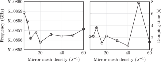
Figure 2. Numerical convergence of the resonance frequency and damping time performed in [6] (the mirror mesh density is labeled in number of mesh elements per wavelength λ).
Download figure:
Standard image High-resolution imageSince we are looking for resonances associated to complex-valued eigenfrequencies, we are led to solve a non-Hermitian eigenvalue problem. Indeed, the equivalent materials introduced to model the unboundedness of the domain (the PML) are non-Hermitian and destroy the Hermitian nature of the initial lossless problem. Unfortunately, it is well known that these problems are hard to solve [25]. Moreover, the FE discretization leads to very large sparse matrices, but, over the last few years, powerful algorithms implemented in open source libraries have been developed [26, 27]. Formally, the complex-valued resonance angular frequency is defined as:
where  is the cavity resonance frequency,
  the damping time and
  the imaginary unit.
All these elements together led us to the proposed numerical model for the computation of the lifetime of a photon in a QED cavity.
3. Computational setup
In this work, we used a homemade high-order FE code4 , which takes advantage of an efficient assembly technique, as described in [28]. Indeed, quite often with high-order techniques, the computational bottleneck is found to be the assembly of the discrete operator itself. It is worth mentioning that the discrete high-order FE spaces used are those proposed in [22]. Regarding the eigenvalue solver, the developed tool relies on the SLEPc library5 [26, 27]. When an LU decomposition has to be carried out (see section 3.5), the MUMPS6 [29, 30] library is called, and is configured for parallel analysis with the ParMETIS7 [31] reordering.
Among the eigenvalues in the  region of the spectrum, we expect to find one with a high ratio between the real and imaginary parts. This eigenvalue corresponds then to a mode where the cavity exhibits a large damping time (or equivalently, a high quality factor): the photon 'trapping' mode. Our objective is to find a numerically converged damping time: i.e. quasi-independent to both an increase of the FE discretization order and the mesh size.
Before going any further, one last point must be raised. Since the mirrors are toroidal, the cavity actually exhibits two resonant modes: one for each radius. They are both TEM900 modes near  and are separated by
  [5, 32]. In the following, these modes will be referred to as polarization 1 and 2.
3.1. Geometry
Let us now discuss the geometry considered for the simulations. In order to reduce the number of unknowns, only one quarter of a single mirror is modeled, as shown in figure 3. Furthermore, the air surrounding the quarter mirror is represented by a rectangular parallelepiped, as shown in figure 4(a). As discussed in section 2, a PML is added to model the surrounding space, as depicted in figure 4(b). As a first guess, the PML thickness is taken as 1λ (where  is the wavelength at
  ), and its distance from the mirror is also set to 1λ. More details on the PML can be found in sections 2 and 3.4.

Figure 3. Geometry of the mirrors.
Download figure:
Standard image High-resolution image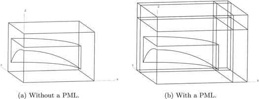
Figure 4. Computational domain.
Download figure:
Standard image High-resolution imageThe final geometry is depicted in figure 4(b), and was generated by the Open CASCADE8 engine. This library was driven using the python9 interface provided by Gmsh10 [33]. Finally, the computational domain is meshed using the Gmsh mesh engine. Since our objective is to use high-order FE discretizations, curved mesh elements are mandatory [34], not only to achieve a precise representation of the curved mirror, but also to keep the number of mesh elements to an acceptable value.
3.2. Eigenvalue problem
Our objective is to find the eigenvalues of the photon cavity. In other words, we need to find every possible value of the angular frequency ω, such that
holds, where  is the speed of light in vacuum,
  the electric field, and where Ω is the computational domain (i.e. the quarter mirror surrounded by the PML). To clarify the presentation, the treatment of the boundary conditions is discussed in the next subsection.
From a FE point of view, this eigenvalue problem writes [35]:
where  is a finite-dimensional subspace (of size N) of
  , the space of square integrable functions with a square integrable curl (these function are also commonly referred to as edge elements). The electrical field
  is then approximated by:
where the coefficients aj are unknown. Thus, the (generalized) eigenvalue problem writes:

By identifying the terms in equation (1), we have:
- the vector
![${{\bf{a}}}_{k}={[{a}_{k,0},...,{a}_{k,N-1}]}^{T}$](data:image/png;base64,iVBORw0KGgoAAAANSUhEUgAAAAEAAAABCAQAAAC1HAwCAAAAC0lEQVR42mNkYAAAAAYAAjCB0C8AAAAASUVORK5CYII=) containing the degrees of freedom for
containing the degrees of freedom for
- the matrix
- the matrix .
![${{\bf{a}}}_{k}={[{a}_{k,0},...,{a}_{k,N-1}]}^{T}$](https://content.cld.iop.org/journals/1367-2630/20/4/043058/revision2/njpaab6fdieqn19.gif)

In this paper, the eigenvalue problem (1) is solved by the Krylov–Schur algorithm [36, 37] from the SLEPc library [26, 27]. The relative tolerance of the eigenvalue solver is set to 10−15.
3.3. Boundary conditions
As motivated above, only one quarter of a single mirror is modeled. To simulate the actual configuration, appropriate boundary conditions have to be imposed on the geometry of figure 4(b). In what follows,  is the unit vector outwardly oriented normal to Ω.
- (i)A zero tangential magnetic field on the Oxy-plane:
- (ii)Depending on whether polarization 1 or 2 is considered.
- Polarization 1: a zero tangential magnetic field on the Oxz-plane, and a zero tangential electric field on the Oyz-plane:
- Polarization 2: a zero tangential magnetic field on the Oyz-plane, and a zero tangential electric field on the Oxz-plane:
- (iii)A zero tangential electric field on the outer boundary of the PML:

Moreover, since the mirror is made of superconducting material, we assume that it has a zero resistivity:

For simplicity, we also consider the frame of the mirror to have a zero resistivity:

3.4. Perfectly matched layer
Let us now specify the PML used for the considered simulations. Since we chose a parallelepiped to surround the mirror, it is a natural choice to use a Cartesian PML [7, 8]. A PML is usually described by its damping functions σx(x), σy(y) and σz(z). In this paper, we chose the following hyperbolic profiles:
where ΔX (or ΔY, or ΔZ) is the thickness of the PML in the x (or y, or z) direction, and where Xmax (or Ymax, or Zmax) is the distance between the center of the mirror and the PML in the x (or y, or z) direction. These profiles are inspired from [38], where a  (with α∈{X, Y, Z}) term is added to remove the jump between the truncated domain and the PML.
From these damping profiles, it is then possible to compute an equivalent relative electrical permittivity and relative magnetic permeability in the PML domain:
where  for all i ∈ {x, y, z}.
3.5. Spectral transform
In our cavity problem, it is not required to extract the entire spectrum of (1): indeed, only the TEM900 mode is of interest. Therefore, a spectral transform is used. The idea is to modify the eigenvalue problem, so that the eigenvalues around a given target are easier to compute [39]. In practice, the shift-and-invert transform [39, 40] is used. That is, instead of solving (1), the following equivalent (from the eigenvalue point of view) problem is solved:
where σ is a well chosen shift and where  . Since the resonance frequency of the cavity is known to be
  [5], the shift σ is taken as:

It is worth noticing that the spectral transform involves an LU decomposition of  , which is handled by the MUMPS library.
4. Three-dimensional high-order FE simulations
With all these tools in hand, let us now discuss some three-dimensional high-order FE simulations. It is worth mentioning that in the following results, some data are missing because of memory limitations (see section 5).
4.1. Solution convergence: mesh density and FE discretization
Based on the computational setup presented previously, a first set of simulations is run in order to assess the numerical convergence of the computed solutions. In practice, five tetrahedral meshes are generated, with 3 to 7 mesh elements per targeted wavelength (i.e.  , as mentioned in section 3). In each case, the mesh exhibits a 3rd-order curvature. From the FE point of view, three discretizations are considered: order 3, order 4 and order 5. Each simulation is carried out with 120 MPI11
processes. Depending on the problem size, these processes are distributed between 5 and 120 computing nodes. On each node,
, as mentioned in section 3). In each case, the mesh exhibits a 3rd-order curvature. From the FE point of view, three discretizations are considered: order 3, order 4 and order 5. Each simulation is carried out with 120 MPI11
processes. Depending on the problem size, these processes are distributed between 5 and 120 computing nodes. On each node,  of memory is available.
For each simulation, three eigenvalues are computed. In each case, only one eigenvalue exhibits a very large damping time and is selected as the resonant one. Figure 5 depicts the numerical convergence of the computed resonance frequencies and damping times for polarization 1.
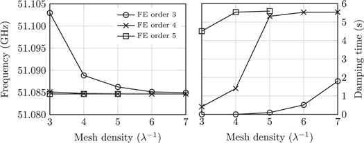
Figure 5. Resonance frequencies and damping times: polarization 1 and 3rd-order mesh elements.
Download figure:
Standard image High-resolution imageFor the resonance frequency, we may conclude that convergence is achieved: the resonance frequency for polarization 1 is found at  . However, for the damping time, convergence is more delicate to assess. Clearly, the 3rd-order simulations did not yet converge. The 4th- and 5th-order simulations seem to converge toward a damping time around
  . More accurate discretizations would of course be welcome, but, due to memory limitations discussed in section 5, these data are not accessible. Nevertheless, a few indicators suggest that the computed damping time will remain in this range. First, the 4th- and 5th-order curves suddenly saturate around
  . Secondly, at a mesh density of 5 mesh elements per wavelength, the damping time varies by only a factor of 5% between the two highest-order solutions. Finally, a variation of only 1% is recorded between the best 4th-order estimate and the 5th-order one.
Compared to the damping time of  determined experimentally, the computed one is 43 times higher. Four major idealizations made in our model could explain this discrepancy. First, our geometry is ideal: the mirrors are exactly toroidal and perfectly aligned. Secondly, our model consists of only the two mirrors floating alone in the void, whereas the mirrors are surrounded by sophisticated equipment in the actual experiment [5], that could introduce additional losses. Thirdly, the residual resistivity of the superconducting material has not been taken into account. Indeed, since we are not operating at absolute zero temperature, some carriers are not in a superconducting state, leading thus to ohmic losses. Furthermore, it can be shown that these losses are increasing with the square of the frequency [41]. And finally, the roughness of the actual mirror is not modeled. As we will see in the following section, this has a dramatic effect on the value of the computed damping time. Let us stress that these issues can be alleviated by technical improvements, while the open nature of the cavity, and the associated computed losses, is an intrinsic property of the device.
To conclude, and for illustration purposes, figure 6 depicts the eigenmode associated to the cavity resonance. For clarity, the vectorial electric field is shown only on the Oxz- and Oxy-planes. It can be directly noticed that this mode exhibits a cylindrical symmetry around the z axis and 4.5 antinodes. Because of the boundary condition on the Oxy-plane, the total number of antinodes is doubled, confirming thus that polarization 1 is a TEM900 mode.
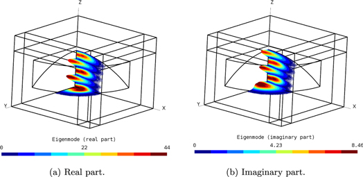
Figure 6. Eigenmode associated with the polarization 1 resonance (field distribution plotted only on the Oxz- and Oxy-planes).
Download figure:
Standard image High-resolution image4.2. Polarization 2
In the previous convergence test, only polarization 1 was considered. Let us now focus on polarization 2. Based on the previous simulations, only the 4th- and 5th-order FE solutions are considered. Figure 7 depicts the computed frequencies and damping times for polarization 1 and 2. In addition, the frequency difference between the two polarizations is provided in table 2.
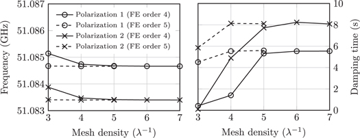
Figure 7. Resonance frequencies and damping times: 3rd-order mesh elements, 4th- and 5th-order finite element discretizations.
Download figure:
Standard image High-resolution imageTable 2. Frequency difference between polarization 1 and 2: 3rd-order mesh elements, 4th- and 5th-order finite element discretizations.
| Frequency difference (MHz) | ||
|---|---|---|
Mesh density 
|
FE order 4 | FE order 5 |
| 3 | 1.2631 | 1.2638 |
| 4 | 1.2659 | 1.2638 |
| 5 | 1.2636 | 1.2639 |
| 6 | 1.2639 | — |
| 7 | 1.2639 | — |
As for polarization 1, we can directly notice that the cavity resonance frequency has numerically converged to  . Moreover, we have reached a frequency difference of
  , which matches the difference measured experimentally [5, 32].
For the damping time, we get a result similar to polarization 1: the computed damping seems to converge toward a value around  . Again, the computed damping time is significantly larger than the measured one. It is worth noticing that the damping time is larger for polarization 2 than for polarization 1. This phenomenon is quite easy to explain, since polarization 2 is associated to the largest radius.
4.3. Mesh curvature
So far, the geometry has been meshed with 3rd-order mesh elements. Let us now analyze the impact of the mesh curvature on the simulations. To do so, only polarization 1 is considered for simplicity. Moreover, we limit ourselves to FE discretizations of order 4. As done previously, the geometry is meshed with a density of tetrahedra varying between 3 and 7 mesh elements per wavelength. However, this time, the geometrical order of the elements ranges between 1 and 4. Figure 8 shows the computed frequencies and damping times.
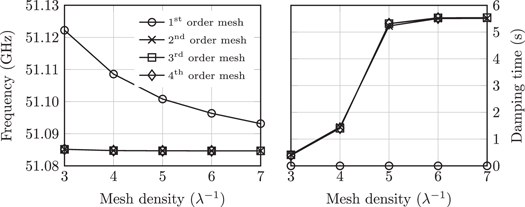
Figure 8. Resonance frequencies and damping times: polarization 1 and 4th-order finite element discretization.
Download figure:
Standard image High-resolution imageBy analyzing the data of figure 8, we can directly notice that the damping time does not converge with 1st-order mesh elements. On the other hand, there is no significant difference between simulations using high-order meshes. Obviously, straight mesh elements fail to compute the cavity damping time. Since the shape of the mirrors is curved, approximating it with 1st-order elements introduces some kind of numerical roughness on its surface. This roughness does not significantly impact the resonance frequency. However, it can lead to unwanted scattering, destroying the stability of the wave. This problem has been noticed in the previous attempt to simulate the photon cavity [6].
A last question remains: can the lack of curvature of the 1st-order mesh elements be compensated by a better mesh refinement of the mirrors? To answer this question, let us setup the following simulations. A mesh with 5 tetrahedra per wavelength is used everywhere in the computational domain, except on the surface of the mirror, where refinements of 5, 10 and 20 elements per wavelength are used. The geometrical order of the mesh ranges between 1 and 4, and a 4th-order FE discretization is used for the computations. Let us note that only polarization 1 is considered. The computed damping times are reported in figure 9.

Figure 9. Damping times: polarization 1, 5 tetrahedra per wavelength (except on the mirror) and 4th-order finite element discretization.
Download figure:
Standard image High-resolution imageBased on the results of figure 9, we can directly notice that increasing the mesh density on the surface of the mirror does not help to achieve convergence for the damping time, at least when straight mesh elements are used. Thus, we can conclude that the damping time is highly sensitive to the numerical roughness introduced by the mesh. Therefore, using curved mesh elements is mandatory to simulate the cavity in order to avoid this virtual roughness.
4.4. Sensitivity of the solution with respect to the PML
Let us now study the sensitivity of the computed solution with respect to the parameters of the PML: its distance from the mirror and its thickness. For this analysis, the following setup is used:
- a tetrahedral mesh of order 4, with a density of 5 mesh elements per wavelength;
- a FE discretization of order 4;
- a PML thickness ranging from 0.25λ to 2λ;
- two distances between the mirror and the PML, 1λ and 2λ.
The computed damping times are shown in figure 10. The mean resonance frequency and the maximum deviation from this mean are given in table 3.

Figure 10. Damping times: polarization 1, 5 mesh elements per wavelength, 4th-order mesh elements and 4th-order finite element discretization.
Download figure:
Standard image High-resolution imageTable 3. Resonance frequency: polarization 1, 5 mesh elements per wavelength, 4th-order mesh elements and 4th-order finite element discretization.
Distance PML-to-mirror 
|
Mean frequency (GHz) | Maximum deviation (GHz) |
|---|---|---|
| 1 | 51.08468 | 2.5 × 10⁻⁶ |
| 2 | 51.08468 | 2.3 × 10⁻⁶ |
Let us start by analyzing the results presented in table 3. Based on the available data, we can conclude that the resonance frequency does not depend on the PML parameters. On the contrary, figure 10 indicates that the damping time is very sensitive to these parameters. Therefore, we cannot conclude that the damping time converged with respect to the PML-to-mirror distance and the PML thickness, since the behavior is too oscillatory. However, the variations of the damping time seem to remain bounded, which indicates that, even though a larger PML (in term of PML-to-mirror distance and thickness) is preferred, the cavity damping lies in the  range.
To conclude this subsection, it is also worth mentioning that two additional numerical experiments were carried out. First, in addition to the boundary condition given in section 3.3 for the PML boundary, we also imposed:
Secondly, in addition to the PML equivalent materials given in section 3.4, we also tested the following constant PML parameter:

In both cases, the same conclusions were drawn. Furthermore, our findings are also supported by additional PML convergence results presented in section 6 for a two-dimensional setup. There, the numerical convergence of the PML is clearly observed, and it is shown that a PML-to-mirror distance of 1λ, as well as a PML thickness of 1λ, already give numerically sharp results.
4.5. Simulation time
To conclude the analysis of our three-dimensional high-order computations, let us give some order of magnitude about the wall clock time taken by the simulations. The smallest simulation (3 mesh elements per wavelength with a 3rd-order FE discretization) counted 517556 unknowns and took less than 1 minute. It was run using 5 computing nodes. On the other hand, the largest simulation (7 mesh elements per wavelength with a 4th-order FE discretization) counted 11443760 unknowns and took less than 11 hours. It was run using 120 computing nodes.
5. Memory scaling
In order to increase the accuracy on the damping time of the previous computations, a higher mesh resolution, FE discretization order and/or PML size are needed. However, for now and with the available computational resources, it is not possible to increase the problem size, since the memory scaling limit of the MUMPS solver seems to be reached.
It is worth noticing that the memory scaling problem is not specific to the MUMPS implementation, but affects the entire family of direct solvers. Another approach would be to use instead a preconditioned iterative method. However, this technique is known to perform poorly for wave problems, at least with classical preconditioners [42]. The design of good preconditioners for wave problems [43, 44] and of memory efficient direct solvers [45] remains an active field of research.
In the following of this section, two examples are discussed to illustrate the memory scaling performance.
5.1. Two fifth-order test cases
Let us look at the two simulations hereafter:
- FE discretization of order 5;
- mesh curvature of order 5;
- two mesh densities, 5 and 6 mesh elements per wavelength;
- polarization 1.
These two simulations led to, respectively, 8019588 and 13363722 unknowns. The test cases were launched on 120 computing nodes, with 64 GB of memory available on each node. The smallest simulation ran successfully, whereas the largest simulation failed because of a memory deficiency during the LU factorization stage. This latter case was run again with 240 nodes but failed for the same reason.
Let us now look at the peak virtual memory allocated by each process for the problem with 8019588 unknowns, as shown in figure 11. Statistics are available in table 4. From these data, we can see that the memory usage is not uniformly distributed across the computing processes. On average, we use 17 GB with a quite low standard deviation. However, we have two spikes above 25.5 GB (i.e. 50% above the mean). It is those spikes that limit the memory scaling of our simulations.
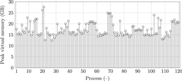
Figure 11. Peak virtual memory allocated per process: 8019588 unknowns, 5th-order case.
Download figure:
Standard image High-resolution imageTable 4. Peak virtual memory allocated: statistics (8019588 unknowns, 5th-order case).
| Mean value | Standard deviation | Maximum value | Minimum value |
|---|---|---|---|
| 17 GB | 3 GB | 28 GB | 13 GB |
5.2. Two fourth-order test cases
Let us take another example:
- FE discretization of order 4;
- tetrahedral mesh of order 4, with a density of 7 mesh elements per wavelength;
- polarization 1.
We ran this setup (11443760 unknowns) successfully on 120 and 240 computing nodes. The peak virtual memory distribution is available in figure 12, and statistics are available in table 5.
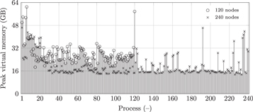
Figure 12. Peak virtual memory allocated per process: 120 and 240 nodes, 11443760 unknowns, 4th-order case.
Download figure:
Standard image High-resolution imageTable 5. Peak virtual memory allocated: statistics (120 and 240 nodes, 11443760 unknowns, 4th-order case).
| Nodes | Mean value | Standard deviation | Maximum value | Minimum value |
|---|---|---|---|---|
| 120 | 28 GB | 7 GB | 61 GB | 17 GB |
| 240 | 19 GB | 7 GB | 46 GB | 13 GB |
From the above results, we have once again some memory spikes far above the mean value. Let us focus only on the two largest spikes: 46 GB (240 nodes) and 61 GB (120 nodes). We can directly notice that by increasing by  the total available memory, the largest spike is decreased by only 25%, thus limiting the scaling performance.
6. Further analysis with a similar two-dimensional model
As we saw in the previous sections, the memory scaling is the main computational bottleneck of our simulations. In order to push our analysis of the photon cavity further, we built a two-dimensional model. Since the mirrors have different curvature radii, our cavity is inherently a three-dimensional structure, and thus cannot be described in two-dimensions. One of the closest two-dimensional counterparts are infinitely long cylindrical mirrors. Note that this is still an open structure and the very same numerical convergence challenges are expected. Therefore, we consider in this section a similar, but not equivalent, model. An alternative model would be to consider two spherical mirrors with a two-dimensional axisymmetric approach. However, this strategy does not exhibit any additional feature in term of open cavity resonances. Furthermore, the three-dimensional spherical mirrors exhibit a degenerated mode, which is not the case with the infinitely long cylindrical version.
The structure studied hereafter consists of two cylindrical mirrors in the Oxz-plane, that extend to infinity along the y axis. The mirrors have a radius of  (the major radius of the three-dimensional cavity). By applying symmetries, in analogy to the three-dimensional numerical setup, our two-dimensional model consists of only one half of a single mirror. Again, PMLs are used to model the infinite domain, as depicted in figure 13. Finally, let us mention that except from the changes mentioned above, the numerical parameters of the three-dimensional cases are reused in the two-dimensional simulations.

Figure 13. Two-dimensional geometry used for the simulations (with PML).
Download figure:
Standard image High-resolution image6.1. Numerical convergence of the damping time
Since our two-dimensional model exhibits fewer unknowns, let us first use larger mesh densities compared to the three-dimensional case, in order to assess the convergence of the damping time. From our previous analysis, we found that 2nd-order mesh elements were sufficient to represent the geometry precisely. Thus only this kind of element is used. The mesh density varies between 5 and 40 mesh elements per wavelength. For the FE discretization, 3rd-, 4th- and 5th-order FE bases are considered. The PML is located at one targeted wavelength of the structure, and its thickness is set to one wavelength. The computed resonance frequencies and damping times are reported in figure 14.
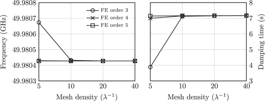
Figure 14. Two-dimensional resonance frequencies and damping times with high-order discretizations.
Download figure:
Standard image High-resolution imageThis figure indicates that the computed resonance frequencies are monotonously converging to  for increasing mesh densities and FE discretization orders. Regarding the computed damping times, the calculated results are also monotonously converging to
  . This value is below the
  found for the three-dimensional polarization 2 case. However, let us recall that this two-dimensional case is modeling a similar, but not equivalent, situation. Furthermore, it is worth mentioning that already with 5 mesh elements per wavelength, with a 4th- or a 5th-order FE discretization, numerically valid damping times are computed. This observation agrees with the analysis performed for the three-dimensional case, and is an additional indicator that the results presented in the sections 4.1 and 4.2 are numerically valid. Finally, it is worth noticing that for both two- and three-dimensional situations, the computed damping time is well above the
  found experimentally. This comforts us in our assumption that the discrepancy between the simulations and the experimental data has to be attributed to our idealizations, rather than in numerical convergence problems.
6.2. Sensitivity of the solution with respect to the PML
Let us now analyze the sensitivity of the results with respect to a variation of the PML thickness and position. In this numerical experiment, the following parameters are used: a mesh density of 5 mesh elements per wavelength, 4th-order mesh elements and a 5th-order FE discretization. Based on the previous analysis, we know that these parameters are sufficiently accurate. In this numerical experiment, both the PML thickness and position (with respect to the mirror) are taken equal and in the  set. This parameter sweep leads to the results presented in figure 15 and table 6.

Figure 15. Two-dimensional resonance frequencies and damping times for a sweep of the PML parameters (both thickness and position are taken equal): 5 mesh elements per wavelength, 4th-order mesh and a 5th-order FE discretization.
Download figure:
Standard image High-resolution imageTable 6. Two-dimensional resonance frequencies and damping times for a sweep of the PML parameters (both thickness and position are taken equal): 5 mesh elements per wavelength, 4th-order mesh and a 5th-order FE discretization.
| Moment | Resonance frequency (GHz) | Damping time (s) |
|---|---|---|
| Mean value | 49.9804 | 7.15 |
| Standard deviation | 2.27 × 10⁻¹⁰ | 1.46 × 10⁻³ |
Based on these data, we can conclude that both the computed resonance frequencies and the damping times are not significantly impacted by a change of the PML parameter. It is however interesting to notice that, as expected, the damping time is more sensitive to a PML variation as compared to the resonance frequency. Again, the numerical stability of the results obtained for this two-dimensional case, with a large PML parameter sweep, comforts us that our three-dimensional simulations are correct. In particular, we can directly notice that numerically valid results can be obtained with a PML-to-mirror distance, as well as a PML thickness, of 1λ.
6.3. Comparison with a first-order finite element simulation
For this numerical experiment, we compared a 1st-order FE method with our high-order simulations. Figure 16 depicts the computed frequencies and damping times for a mesh density ranging from 5 to 320 straight mesh elements per wavelength. As expected (based on our three-dimensional analysis), the virtual roughness introduced by the straight mesh significantly impacts the numerical results. Indeed, we need at least 160 mesh elements per wavelength to reach a value close to the expected value of  .
.
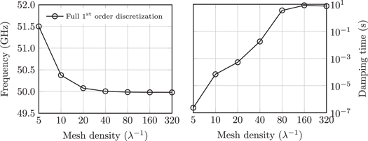
Figure 16. Two-dimensional resonance frequencies and damping times with a 1st-order FE method on straight meshes.
Download figure:
Standard image High-resolution imageIt is worth noticing that the largest simulation setup leads to 20363036 unknowns, corresponding to a linear system with twice the size of the largest three-dimensional case. Nevertheless, this simulation does not suffer the same memory limitations. This phenomenon is easily explained by the better non-zero structure of the matrices of the two-dimensional computations, resulting in a lower fill-in.
6.4. Simulation time
In this section, let us compare the computation time taken by different mesh densities and FE discretization orders. The results are summarized in table 7. As can be noticed directly, the computation time can be reduced by increasing the FE discretization order and decreasing the mesh density at the same time (while keeping the accuracy constant). This leads to a reduction of the number of unknowns, and thus a decrease of the computation time.
Table 7. Computation time for different parameters with the two-dimensional model.
| Order | |||||
|---|---|---|---|---|---|
| FE (–) | Mesh (–) | Mesh density 
|
Unknowns (–) | Comp. time (s) | Damping (s) |
| 1 | 1 | 320 | 20363036 | 2682 | 7.43 |
| 2 | 2 |

|

|

|
7.17 |
| 3 | 2 |

|

|

|
7.16 |
| 4 | 2 |

|

|

|
7.16 |
| 5 | 2 |

|

|

|
7.15 |
6.5. Other modes
For this last part of our two-dimensional simulations, we computed the resonance frequency and the associated damping time for the other 'trapping' modes of the cavity. Based on our previous convergence analysis, we chose to use a 5th-order FE discretization. The mesh exhibits a density of 10 mesh elements per targeted wavelength and a 2nd-order curvature. It is worth stressing that, since the resonance frequencies are different for each mode, the meshes are also different. This is also the case for the actual length of the PML and its distance to the mirror. Let us also note that because of the symmetry conditions, only the odd modes were computed.
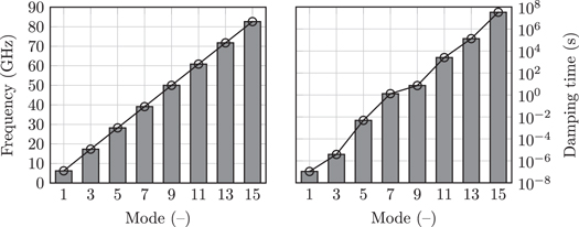
By analyzing the results displayed in figure 17, we can directly notice the linear dependence of the resonance frequency on the mode number. This can be also observed for the damping time in a logarithmic scale, with the notable exception of the transition between the 7th and the 9th modes, where the slope suddenly decreases. It is worth noticing that, after a deeper investigation, this phenomenon does not seem to come from a numerical problem. Finally, let us recall that in our simulations, the surface resistivity of the superconducting mirrors was neglected. However, this parameter is expected to limit the damping time increase with the mode number, since it grows with the frequency [41].
Figure 17. Photon trapping modes calculated for the two-dimensional model.
Download figure:
Standard image High-resolution image
7. Conclusion
In this paper, we simulated the photon cavity designed by Serge Haroche and his coworkers, for recording the birth and death of a photon, by using the classical electromagnetic theory, PMLs, and the finite element method. This problem has already been treated in the literature with straight tetrahedral meshes and a second-order finite element discretization. Unfortunately, the authors were not able to compute the damping time, because of its high sensitivity with respect to the mesh refinement.
In this work, we improved the computations substantially, by using curved mesh elements combined with finite element discretizations of high orders. We demonstrated that they are mandatory for tackling the computation of the damping time of the photon cavity, since they alleviate both the virtual roughness introduced by the mesh and the pollution effect impacting time-harmonic wave problems. We also showed that computing the damping time of the cavity is computationally demanding, and pushes the direct solvers and modern computing facilities to their limits. Nevertheless, a satisfactory convergence study was performed in two steps. First, the convergence of the damping time has been established on the basis of a few points in a three-dimensional setup. Then, a two-dimensional model, exhibiting the same behavior as its three-dimensional counterpart, has been studied. By enabling finer discretizations, this additional analysis consolidated the numerical validity of the three-dimensional model. Furthermore, thanks to the two-dimensional model, we showed that a classical first-order finite element approach requires at least 160 mesh elements per targeted wavelength in order to reach a sufficient accuracy, whereas a fifth-order discretization gives the same accuracy with only 5 second-order mesh elements per wavelength.
The computed damping times, with either a three- or a two-dimensional approach, are significantly higher than the one found experimentally: the simulations suggests a damping time of about 5.6 s or  , depending on the polarization, whereas the experiment shows a damping time in the
  range. This discrepancy is explained by the simplifications made in our model: we indeed focused only on the losses introduced by the open nature of the cavity. Among these idealizations, (i) we considered perfectly aligned and exactly toroidal mirrors; (ii) we assumed that the two mirrors are floating alone in the void; (iii) we neglected the residual resistivity of the superconducting material; (iv) we did not consider the surface roughness. It is worth noticing that these issues can be alleviated, e.g. by technological improvements in manufacturing and material science. On the other hand, the open nature of the cavity is intrinsic to the device.
Acknowledgments
This work has been supported by the Belgian Science Policy Office (BELSPO) under Grant IAP P7/02 and the ANR RESONANCE project, grant ANR- 16-CE24-0013 of the French Agence Nationale de la Recherche. The computational resources have been provided by the Consortium des Équipements de Calcul Intensif (CÉCI), funded by the Fonds de la Recherche Scientifique de Belgique (F.R.S.–FNRS) under Grant 2.5020.11. Furthermore, this work has benefited from computational resources made available on the Tier-1 supercomputer of the Fédération Wallonie–Bruxelles, infrastructure funded by the Walloon Region under the grant agreement 1117545. The work of N Marsic has been supported by the Belgian Research Training Fund for Industry and Agriculture (FRIA). Finally, the authors would like to express their gratitude to the referees for their constructive comments, and to Michel Brune (Laboratoire Kastler Brossel, CNRS, ENS, UPMC, Collège de France) for the picture of the mirrors, shown in figure 1, and his valuable feedback on the manuscript.
Footnotes
- 4
Available from the Gmsh repository (http://gitlab.onelab.info/gmsh/small_fem); let us note that this software is a general purpose FE library, and not a dedicated solver for our cavity problem.
- 5
Available at: http://slepc.upv.es
- 6
Available at: http://mumps-solver.org
- 7
ParMETIS is a graph partitioner, used by MUMPS for minimizing the fill-in, by reordering the matrix terms; ParMETIS is available at: http://glaros.dtc.umn.edu/gkhome/metis/parmetis/overview
- 8
Available at: http://opencascade.com
- 9
Available at: http://python.org
- 10
Gmsh is a three-dimensional FE mesh generator with built-in pre- and post-processing facilities; available at: http://gmsh.info
- 11
The message passing interface (or MPI) is a standard describing a message-passing system allowing computer processes to exchange data; more details can be found at: http://mpi-forum.org/