

Abstract
Forest degradation is widespread around the world, due to multiple factors such as unsustainable logging, agriculture, invasive species, fire, fuelwood gathering, and livestock grazing. In the Brazilian Amazon forest degradation from August 2006 to July 2016 reached 1,1 869 800 ha. The processes of forest degradation are still poorly understood, being a missing component in anthropogenic CO2 emission estimates in tropical forests. In this work, we analyzed temporal trajectories of forest degradation from August 2006 to July 2016 in the Brazilian Amazon and assessed their impact on the regional carbon balance. We combined the degradation process with deforestation-related processes (clear-cut deforestation and secondary vegetation dynamics), using the spatially-explicit INPE-EM carbon emission model. The trajectory analysis showed that 13% of the degraded area ended up being cleared and converted in the period and 61% of the total degraded area experienced only one event of degradation throughout the whole period. Net emissions added up to 5.4 GtCO2, considering the emissions from forest degradation and deforestation, absorption from degraded forest recovery, and secondary vegetation dynamics. The results show an increase in the contribution of forest degradation to net emissions towards the end of the period, related to the decrease in clear-cut deforestation rates, decoupled from the forest degradation rates. The analysis also indicates that the regeneration of degraded forests absorbed 1.8 GtCO2 from August 2006 and July 2016—a component typically overlooked in the regional carbon balance.
Export citation and abstract BibTeX RIS

Original content from this work may be used under the terms of the Creative Commons Attribution 4.0 license. Any further distribution of this work must maintain attribution to the author(s) and the title of the work, journal citation and DOI.
1. Introduction
Forest degradation carbon emissions are still poorly quantified, although climate change mitigation schemes, such as the UN-led Reducing Emissions from Deforestation and Forest Degradation (REDD +), will require accurate estimates of carbon emissions following forest disturbance (Olander et al 2008, Aragão and Shimabukuro 2010, Rappaport et al 2018, Maxwell et al 2019). In general terms, forest degradation is a reduction in the capacity of a forest to produce ecosystem services such as carbon storage and wood products as a result of anthropogenic and environmental changes (Thompson et al 2013). It is a process with a broad distribution in the global forests and is one of the major responsible of biodiversity loss (IPBES 2019), due to multiple factors such as unsustainable logging, fire, agriculture, invasive species, firewood gathering, and livestock grazing. In this paper, we limit the analysis of forest degradation to the occurrence of forest fires and disordered selective logging activities and assess the possible impacts on annual emissions of greenhouse gases.
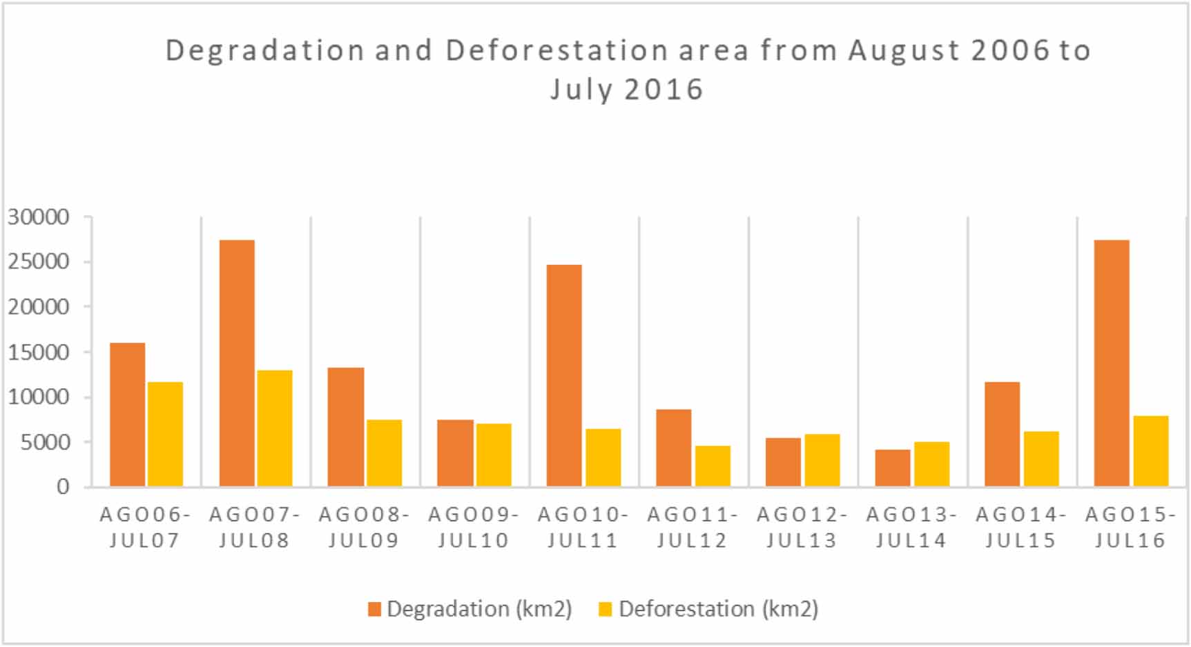
In the Brazilian Amazon, forest degradation is mostly associated with logging and fire, or a combination of both (Nepstad et al 1999, Cochrane et al 1999, Barlow et al 2003, Asner et al 2006, Aragão and Shimabukuro 2010, Alencar et al 2011, Berenguer et al 2018). In the last years, forest degradation has shown significant values, frequently higher than deforestation (INPE 2020). In dryer years, such as 2007, 2010, and 2015, the total degradation area reached over 2000 000 ha (figure 1). The processes leading to degradation impact biodiversity (Barlow and Peres 2008, Berenguer et al 2018), carbon stocks(Gerwing 2002, Foley et al 2007, Blanc et al 2009, Anderson et al 2015, Lennox et al 2018, Silva et al 2018) and increase forest vulnerability to future burning (Nepstad et al 1999).

Figure 1. Forest degradation (orange) and clear cut deforestation (yellow) annual rates as estimated by the PRODES and DEGRAD monitoring systems.
Download figure:
Standard image High-resolution imageAccording to (Rappaport et al 2018), the type of degradation, its frequency, timing, and severity influence changes in the biomass. Therefore, to quantify the carbon emissions derived from forest degradation, it is important to depict its pathways. This knowledge allows us to assess the impact of the different patterns of land cover changes in carbon accounting systems. (Santos et al 2001) mapped and followed the evolution of polygons of logging between 1988 and 1998, leading to clear cutting or forest regeneration, using remote sensing techniques. Of the total area of 17 146 km2, mapped in the Brazilian Amazon, 15.6% were converted into clear-cut deforestation, 43.5% were characterized as degraded forest, and 40.9% regenerated the vegetation cover. (Kury 2016) performed a similar analysis, tracing trajectories from degradation started at 2006. The results pointed out that, of the areas designated as degraded in 2006, 21% were converted into clear-cut by 2012 and 31% followed a trajectory of more degradation events. In the remaining area (48% of the area), no new degradation events or clear-cut occurred.
In this paper, we trace degradation trajectories in the Brazilian Amazon from August 2006 to July 2016 to analyze the degradation dynamics, based on (Santos et al 2001) and (Kury 2016). Then, we adapted the degradation component of the spatially-explicit INPE-EM carbon emission model (Aguiar et al 2016) to represent biomass changes following degradation events and assess their impact in the carbon balance.
2. Methods
2.1. Degradation and clear-cut data
We used the DEGRAD system (INPE 2020) as our source of old-growth forest degradation information. DEGRAD is an operational system that identifies old-growth forest areas exposed to forest fires and disordered selective logging. The system is a complement to the PRODES system, also developed by (INPE 2020) that identifies the total removal of vegetation (clear-cut deforestation) in old-growth forest areas.
The mapping of the degraded areas is performed independently each year, without removing areas identified as degraded in the previous years from the analysis. Thus, the DEGRAD system allows assessment of areas that are in the process of regeneration after the degradation event—as well as those in which this degradation is recurring. Therefore, we can consider the information provided by the DEGRAD system in a given year as the indicator of an on-going degradation process caused mostly by fire or logging activities, although some natural disturbance events cannot be differentiated from anthropogenic ones by the DEGRAD product.
PRODES and DEGRAD systems generate annual products based on Remote Sensing images acquired from August of the previous year to July. Therefore, our analysis and estimates of emissions in 2007, for example, refer to the period from August 2006 to July 2007 as they are inferred using PRODES/DEGRAD products. Our analysis covers the period from August 2006 to July 2016. Figure 1 presents the annual forest degradation and deforestation rates as estimated by the two systems. In terms of extension, the PRODES and DEGRAD system only monitor old-growth forests. Once an area is clear-cut, it is not monitored in the following years, even when these areas are eventually abandoned, giving way to secondary forests. Future land cover changes in these areas are monitored by a third INPE system, called TerraClass.
2.2. Degradation trajectories
The trajectories area built by analyzing the fate of all polygon identified by DEGRAD in a given year (the trajectory initial reference year). We intersect them with the DEGRAD and PRODES polygons in the following years, looking for overlaps. As a result, we identified three degradation trajectories
- Degradation to Clear Cut Trajectory: areas identified by the DEGRAD system in a reference year (e.g. 2007) that ended-up being fully cleared and converted (i.e. as detected by PRODES) in any of the following years.
- Multiple Degradation Events Trajectory: areas under recurrent degradation (detected by DEGRAD at least in two distinct years), but that was not fully cleared during the analyzed period.
- Single Degradation Event Trajectory: degradation polygons identified in the reference year that did not intersect with any other degradation or clear-cut polygons in subsequent years.
Polygons identified as part of the trajectory were not considered for the following reference years to avoid double-counting. For example, a polygon observed by DEGRAD 2007 and DEGRAD 2008 is considered part of the 2007 Multiple Degradation Events Trajectory, and discarded from the 2008 trajectory analysis.
2.3. INPE-EM modeling approach
We used the INPE-EM carbon emission model to estimate the CO2 balance for the Amazon region until 2016, considering the clear-cut deforestation and forest degradation processes. INPE-EM (Aguiar et al 2012, Aguiar et al 2016) combines spatially explicit maps of biomass and land cover changes in three distinct components: (a) clear-cut deforestation, (b) secondary vegetation, and (c) forest degradation, to represent emission processes in an integrated way. INPE-EM is based on the bookkeeping model proposed by (Houghton et al 2000) and aims to generate annual estimates of emissions of greenhouse gases (GHG) by land cover change in a spatially explicit way. This model estimates 1st order emissions that assume that all emissions occur at the time of the land cover change and 2nd order emissions, used in this paper, which represent the gradual process of liberation and carbon absorption as occurs in fact. These 2nd order emissions estimates have an attenuated response in relation to land cover changes and carry the influence of lagged emissions due to historical processes that occurred in previous years.
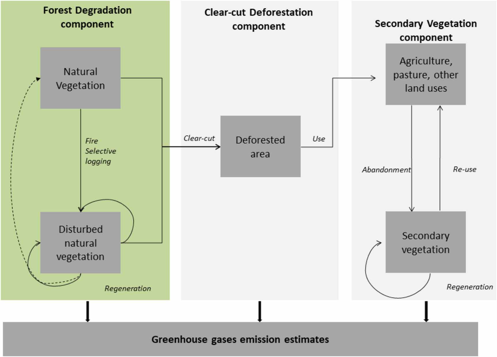
INPE-EM Vegetation Removal Component calculates 1st order and 2nd order emissions due clear cut deforestation. Second order estimate represents the carbon release rate into the atmosphere over time (figure 2), considering that part of the biomass is converted into wood products, part is burned, and part is left on the ground, suffering gradual decomposition (above or below ground). In addition to gross emissions derived from clear cut deforestation of pristine areas, INPE-EM calculates net emissions that combines the dynamics of secondary vegetation in deforested areas. The secondary vegetation component works independently, estimating the dynamics not in the old-growth forest areas, but only in deforested areas, considering the abandonment cycle (regrow and cut) of the secondary vegetation. We used TERRACLASS land use and cover data (IPBES 2019) to estimate the secondary vegetation growth in the model.

Figure 2. INPE-EM model diagram.
Download figure:
Standard image High-resolution imageAdditionally, the biomass stock can increase or decrease according to degradation events. The INPE-EM degradation component, introduced by Aguiar et al (2016) calculates CO2 emission and absorption, dynamically altering the biomass of the old-growth forest areas as the result of degradation events and post-event regeneration. Thereby, it captures both the short-term (carbon release and uptake) and long-term effects (changes in carbon stock due to forest regeneration after the disturbance) of the degradation process. After computing the total amount of lost biomass and consequent CO2 emission in a given year, the model allows for the regeneration of the aboveground live biomass (AGB), assuming the original value will be reestablished after a given number of years, with a constant growth rate, in the original version of the model. The CO2 absorption is calculated considering this growth rate and the forest area remaining in each spatial aggregation unit (cell).
We modified the original version of the INPE-EM degradation component to improve the representation of the biomass changes following a degradation event. We adapted this component to permit the use of different growth curves to represent the regeneration of the AGB and allow the use of multiple AGB loss factors in the same model. This modification allowed us to describe how distinct elements influence the changes in biomass during degradation events, such as its recurrence.
2.4. INPE-EM parametrization
The model was run from 1960 to 2016 to take into account historical emissions of land cover change in Amazonia. A relatively long time interval is necessary to represent the gradual process of carbon liberation and absorption throughout the years. Thereby, present emissions carry the influences of historical land-use processes, and contemporary processes will influence future carbon emissions.
We used 50 × 50 ha cells to represent the spatial variables in the model. In this paper, we used INPE-EM non-spatial mode from 1960 to 2006 and spatial mode from 2007 to 2016. Spatial data is available from 2007 to 2016. To account for lagged emissions and historical disturbances in the biomass, we used historical non-spatial data, based on the literature (table 1) for the 1960 to 2006 period, following the approach adopted in (Aguiar et al 2012). In the INPE-EM model the non-spatial models equivalent to using a single cell for the entire area, which is added to the results of the spatial mode (Aguiar et al 2012). If, on the one hand, this adds uncertainties related to the absence of spatial data for the historical period, on the other hand this procedure allows us to estimate the impact of emissions from past processes on current emissions. Table 1 describes the parameters settings for the INPE-EM degradation component.
Table 1. Parameters settings for the INPE-EM degradation component.
| Parameter | Description | Non-spatial | Spatial |
|---|---|---|---|
| Biomass | Average biomass in a cell unit | 233 MtCO2 ha−1 | Brazilian Third National GHG Inventory (Brazil 2016) |
| Degradation | Percentage of cell unit identified as degraded that year by fire/logging events | 155 872 ha (Santos et al 2001) | DEGRAD/INPE |
| AGB loss | Percentage of AGB lost as result of the event | 54,2% (Rappaport et al 2018) | 54,2% and 83% (Rappaport et al 2018) |
| BGB loss | Percentage of BGB lost as result of the event | 0 | 0 |
| Dead wood loss | Percentage of dead wood lost as result of the event | 0 (Berenguer et al 2014) | 0 (Berenguer et al 2014) |
| Litter loss | Percentage of litter lost as result of the event | 0 (Berenguer et al 2014) | 0 (Berenguer et al 2014) |
| Growth curves | Rates of regeneration of the AGB along the years | Based on (Rappaport et al 2018) relationship between intact and 1x burned forests | Based on (Rappaport et al 2018) relationship between: (a) intact and 1x burned forests, (b) intact and 2x burned forests |
We adopted the biomass spatial data from the Brazilian Third National GHG Inventory (Brazil 2016). The average AGB used for the historical period before the availability of spatial data was 233 Mt CO2 ha−1, corresponding to the average of AGB in the degraded areas for the spatial period considered, according to the National Inventory of GHG emissions (Brazil 2016). We used the DEGRAD System to provide degradation data for the INPE-EM spatial mode. For the non-spatial mode, we used the results of (Santos et al 2001), who assessed an area of 1 714 600 ha degraded forests in the Brazilian Amazon between 1988 and 1998. We considered homogeneous annual average value (155 872 ha) for the period from 1988 to 2006. No degradation was considered before this period (1960–1987), following (Aguiar et al 2016).
We used the relationship between intact and degraded forests over the years described by (Rappaport et al 2018) to represent the biomass loss and recovery in a degraded area. Their results presented the biomass changes following conventional logging and fire pathways. We adopted the '1 time burned (average)' for the historic period. For the spatial mode we combined '1 time burned (average)' e '2 times burned' relations. We based on it to define the AGB loss and generate the AGB regeneration curves.
Since the degradation polygons are frequently smaller than spatial model resolution, the information about the recurrence of degradation in a cell is not enough to decide which relations between intact and degraded forests to use. To improve this relation, we combined this information with the results of the trajectories analysis, presented in section 2.2. If the cells showed degradation recurrence and more than 50% of its degradation fits on the Multiple Degradation Events Trajectory, the model adopted '2 times burned' relations (Rappaport et al 2018) to define AGB loss and AGB regeneration curves for this cell. Otherwise, the model uses the '1 time burned (average)'. The other model parameters were based on (Aguiar et al 2016) and are available in the supplementary material (available online at stacks.iop.org/ERL/15/104035/mmedia).
3. Results
3.1. Trajectories distribution
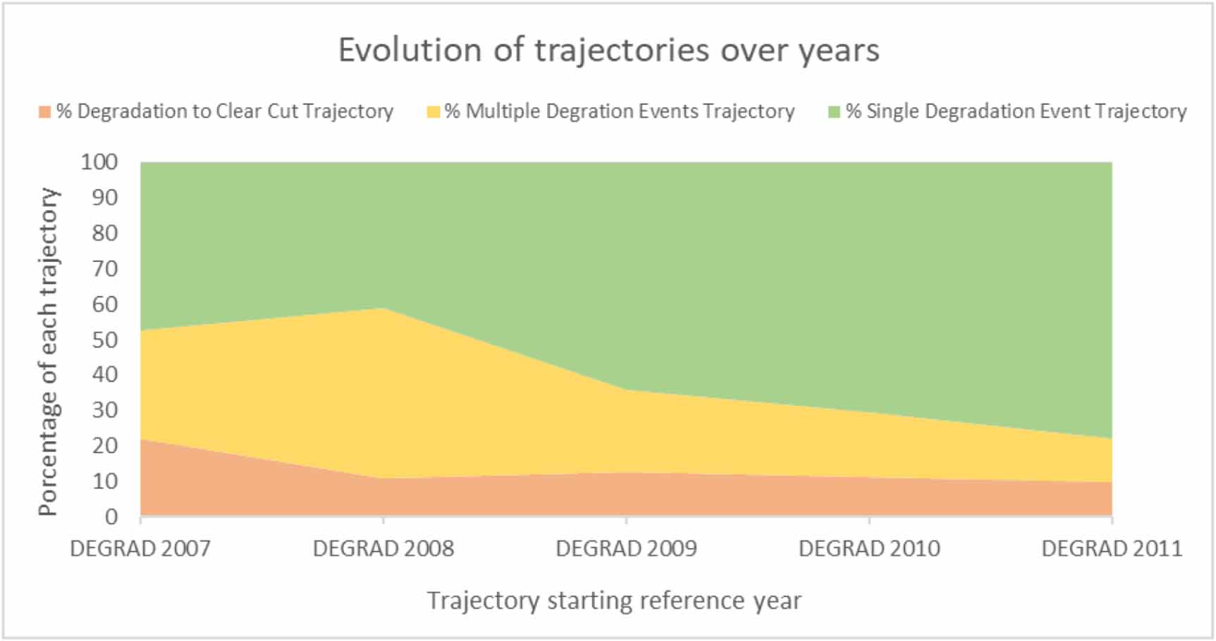
The trajectory analysis shows that the Single Degradation Event Trajectory is prevalent in the Amazon, during all the analyzed period covering 61% of the total degraded areas in a regeneration path without subsequent disturbances in the following 10 years. Although in this section we focus on trajectories starting from DEGRAD 2007 (August 2006–July 2007) to DEGRAD 2011 (August 2010–July 2011) we observed this trend throughout the other years (supplementary material).
Analysis of the evolution of trajectories shows a substantial increase in the Single Degradation Event Trajectory since DEGRAD 2010, reaching more than 70% of the total (figure 3). Contrastingly, our analysis also show that 13% are on the Degradation to Clear Cut Trajectory—a tendency observed since DEGRAD 2008. The other 26.5% of areas are part of the Multiple Degradation Events Trajectory, with recurring events of fire or logging.
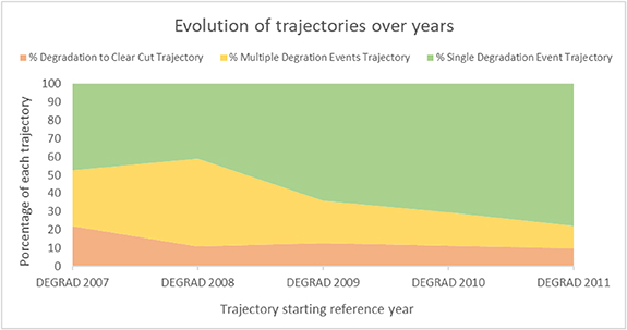
Figure 3. Temporal distribution of degradation to clear cut trajectory the (orange), single degradation event trajectory (green) and multiple degradation events trajectory (yellow).
Download figure:
Standard image High-resolution imageFigure 4 illustrates the heterogeneous spatial distribution of the three trajectories. The Single Degradation Event Trajectory was found all over the Amazon, widely scattered in remote areas, although more concentrated closer to previously opened areas and to the new deforestation frontiers. The Multiple Degradation Events Trajectory was found in areas with high levels of historical deforestation, mainly in Mato Grosso and Tocantins States. Degradation to Clear Cut Trajectory appears close to previously opened deforested areas, expanding towards the Central Amazon from the south.

Figure 4. Spatial distribution of the three trajectories of this study for the period August 2006 to July 2016.
Download figure:
Standard image High-resolution image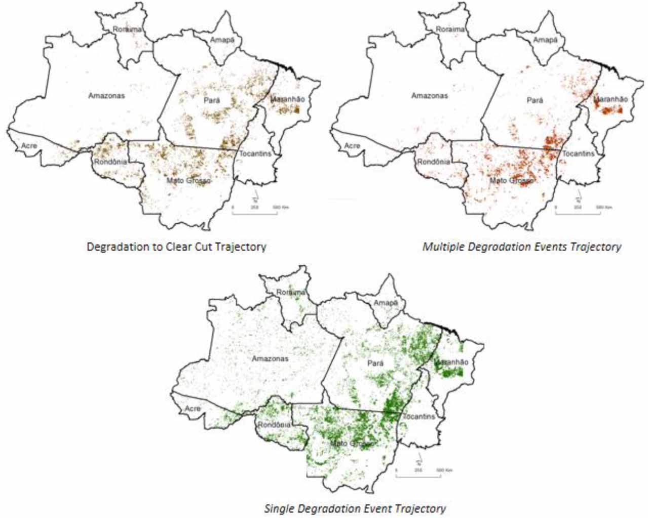
3.2. CO2 emission estimates
The INPE-EM model allowed us to estimate the carbon balance in an integrated way and to assess the impact of the degradation process on it. Within the entire model period, CO2 net emissions totaled 34.943 Gt CO2, considering the emissions from forest degradation and deforestation, absorption from degraded forest recovery, and secondary vegetation growth and emission from the cut of secondary vegetation. The results show an increase in the contribution of forest degradation to net emissions. While degradation (emission and absorption presented in table 2) corresponds to 1.3% from 21.9 Gt CO2 net emissions from 1981 to 2006, it corresponds to 16.2% from 5.4 Gt CO2 emitted from 2007 to 2016.
Table 2. Carbon balance for the Brazilian Amazon from 2007 to 2016 (lagged processes since 1960 due to degraded areas regeneration and secondary vegetation regrowth in clear cut areas).
| CO2 Emissions (Mt Co2) | CO2 Absorption (Mt Co2) | ||||||
|---|---|---|---|---|---|---|---|
| Secondary | Secondary | Degraded | Gross | ||||
| vegetation | vegetation | forest | Emission | CO2 Balance | |||
| Year | Deforestation | cut | Degradation | growth | recovery | (Mt CO2) | (Mt CO2) |
| 2007 | 807 | 89 | 317 | −156 | −32 | 1213 | 1026 |
| 2008 | 748 | 93 | 499 | −161 | −214 | 1340 | 965 |
| 2009 | 633 | 98 | 190 | −164 | −230 | 921 | 527 |
| 2010 | 555 | 103 | 157 | −166 | −196 | 815 | 454 |
| 2011 | 492 | 107 | 395 | −168 | −182 | 994 | 644 |
| 2012 | 413 | 110 | 159 | −169 | −233 | 682 | 280 |
| 2013 | 381 | 114 | 97 | −170 | −215 | 592 | 206 |
| 2014 | 348 | 119 | 78 | −172 | −183 | 545 | 191 |
| 2015 | 343 | 123 | 180 | −173 | −165 | 646 | 308 |
| 2016 | 369 | 127 | 622 | −174 | −172 | 1118 | 771 |
| Total 2007–2015 | 5089 | 1083 | 2694 | −1673 | −1822 | 8866 | 5372 |
| Total 1981–2006 | 22 851 | 1265 | 806 | −2484 | −523 | 24 922 | 21 910 |
| Total 1960–1980 | 7952 | 84 | 0 | −371 | 0 | 8036 | 7661 |
Table 2 shows the estimates of CO2 emissions divided into three periods: (a) from 1960 to 1980, (b) from 1981 to 2006, and (c) from 2007 to 2016. Although all the period before 2007 considered historical non spatial data, 1981–2006 included forest degradation process, while 1960–1980 period only estimated emissions from clear cut deforestation. We emphasize that, as we used PRODES and DEGRAD as our spatial deforestation and degradation source data, 2007 for example, refers to the period from August 2006 to July 2007. The annual estimates from 1960 to 2016 are available in supplementary material.
Our results indicate the increasing importance of degradation in CO2 gross emissions. Forest degradation emissions add up to 0.8 Gt CO2 from 1981 to 2006, while between 2007 and 2016, they were 2.7 Gt CO2. Of the total of 24.9 Gt CO2 of gross emissions from 1981 to 2006, the degradation corresponds to 3.2%, whereas clear cut deforestation shares to 91.7% (22.9 Gt CO2). However, degradation is responsible for 30.4% of the 8.9 Gt CO2 gross emissions between 2007 and 2016. In the same period, clear cut deforestation share decreased to 57.4% (5.1 Gt CO2).
The aggregate effects of the post-disturbance regeneration partially offset these emissions. The CO2 absorption due to degraded forest recovery from 1981 to 2006 was 0.5 Gt CO2, which amount 64.9% of the 0.8 Gt CO2 emitted due degradation in the same period. This proportion is 67.6% when we consider the period from 2007 to 2015 (2.7 Gt CO2 emitted due forest degradation and 1.8 Gt CO2 absorbed due to degraded forest recovery).
4. Discussion
The INPE-EM model allowed us to estimate the net carbon balance in an integrated way and assess the impact of the degradation process on it. We link the analyses of the three trajectories of forest degradation in the Brazilian Amazon to the INPE-EM results, discussing the results in the context of previous studies.
4.1. Trajectories of forest degradation
The increasing dominance of the Single Degradation Event Trajectory points to the significance of isolated degradation events spread all over the Amazon (figure 3). While this trajectory represents 47.5% of the fate of degraded areas identified by DEGRAD 2007, very similar to the results pointed out by (Kury 2016), its share increased in the following reference starting years. For example, for the degraded areas identified by DEGRAD 2010, 70.6% belonged to this category. Spatial pattern of Single Degradation Event Trajectory (figure 3) possibly indicates that those events are not merely linked to anthropic factors. Although this degradation can also indicate non-anthropic disturbances, it requires more investigation to pinpoint how much of that might be due to natural phenomena such as climate events which cause forest blowdowns (Negrón-Juárez et al 2018). (Aragão et al 2018) highlighted the influence of severe droughts in the increase of Amazon forest fires, although our results show the prevalence of Single Degradation Event Trajectory even in non-drought years.
At the same time, our trajectory results also show a slight decrease in the share of the Clear-cut trajectory. While for degraded areas identified in DEGRAD 2007 represented 22% of their fate, after DEGRAD 2008 its share stabilized around 11%. This trajectory shows a concentrated spatial pattern close to previously deforested areas, indicating the initial stages of the clear-cut deforestation process (Pinheiro 2015). Two interlinked factors may explain the decrease in the temporal share of this trajectory. First, the sharp decrease in deforestation rates from 2006 to 2014 is not observed in the temporal evolution of forest degradation rates (figure 1). Second, the increase of scattered degradation events discussed above. This decoupling of deforestation and forest fires events have been reported in the literature before (Aragão et al 2018).
The trajectory of repeated degradation events within a 10 year period, Multiple Degradation Events Trajectory, was found in areas with high levels of historical deforestation, mainly in Mato Grosso and Tocantins States. These areas represent the most degraded and vulnerable forests.
4.2. How these different trajectories impact net CO2 emissions?
The decoupling between deforestation and forest fires observed in the trajectory analysis can also be seen in the CO2 emissions estimated in the INPE-EM model. Our results indicate that forest degradation contribution to the gross emissionsincreased from 3.2% (from 1981 to 2006) to 30.3% (from 2007 to 2016). On the other hand, deforestation contribution decreased from 91.7% to 57.4%. The decrease in Brazilian Amazon deforestation rates since 2004 contributed to this situation (figure 1). Although our results show expressive degradation emissions in the carbon balance, its values presented lower values than deforestation emissions even in dryer years, which agrees with the results obtained by Aguiar et al (2016) and Aragão et al (2014). However, there is enormous uncertainty about the future of these processes. Evidence of an increase of droughts due to climate change (Marengo et al 2018), associated with the recent rise of clear-cut deforestation rates (INPE 2020), pose considerable threats to the region, with potential feedback on the global climate.
The prevalence of the Single Degradation Event Trajectory highlights the importance of considering the absorption by degraded forest recovery in the carbon balance in the Brazilian Amazon. Although the prevalence of this trajectory can have positive effects on the carbon balance compared to the other trajectories, degradation events drastically affect biodiversity (IPBES 2019). These events may drive long term consequences altering forest structure and composition, leading to the impoverishment of forests and further increase flammability for several years (Barlow and Peres 2008). The pulverized pattern observed in the Single Degradation Event Trajectory contributes to more areas throughout the Amazon being exposed to these forest degradation impacts.
4.3. Carbon balance in relation to previous studies
Studies estimating carbon emissions from multiple land cover change processes are becoming more common. For example, (Tyukavina et al 2017) pointed that by 2013, secondary vegetation deforestation, together with old growth forest degradation became comparable to clear cut deforestation. (Aragão et al 2018) also pointed to the growing contribution of forest degradation to gross emissions. Their results indicated that gross emissions derived by wildfire corresponds to more than 50% of those from forest deforestation during drought years. Our results show proportions varying from 37.2% to 55.6% between degradation and gross emission in dryer years (see table 2). However, we only considered the degradation in old growth forests. On the other hand, both (Tyukavina et al 2017,Aragão et al 2018) did not consider the absorption due to the regeneration of degraded old-growth forests.
(Baccini et al 2017) estimated net emissions considering forest growth and losses result from deforestation and forest degradation. Their results indicated 324.8 MtCO2 year−1. Our results pointed 537 MtCO2 year−1 in the same period. Two factors can explain this difference. First (Baccini et al 2017) analyzed only AGB, whereas our model also considers belowground biomass, litter and dead wood. Second, our model considers the historic process evolving land change dynamic and some lagged emissions such as wood products, not estimated by (Baccini et al 2017).
Aguiar et al (2016) also calculated net emissions considering deforestation and forest degradation dynamics, using the INPE-EM model. The positive variation verified in our degradation emission is probably due to the AGB loss factor. We adapted INPE-EM to work with two AGB loss factors to represent the impact of recurrent degradation within a cell in the model. On the other hand, the refinement of regrowth curves to represent the degraded forest regeneration lightly attenuated our degradation absorption estimates in relation to Aguiar et al (2016).
4.4. Uncertainties, limitations and future research
Although the processes of forest degradation are still poorly understood in the Brazilian Amazon, recent efforts are contributing to advance the understanding through field observation (Berenguer et al 2014, Anderson et al 2015, Berenguer et al 2018, Rappaport et al 2018, Withey et al 2018). Such efforts are essential to better represent the forest degradation processes in greenhouse gases models. AGB losses due to the degradation are one of the main uncertainties in the model. We used our trajectories analysis to decrease this uncertainty by combining trajectories information with degradation recurrence within a cell to decide which AGB losses and regrowth curves assume in each case.
Another improvement for future work relates to the trajectories definition. We used 10 year period since we are aware that the longer the interval, the larger the chance of capturing multiple events. However, this should reduce the comparable intervals within each trajectory. Although DEGRAD data is only available from 2007 to 2016, data from other systems could be combined, for example, from the DETER B system (INPE 2020).
Despite the uncertainties associated with the fact that there is no spatial data for the historical period, our results show the importance of including the legacy emissions in the analyzes related to the carbon balance.
5. Conclusion
The INPE-EM model made possible an integrated analysis of the CO2 emissions and absorptions from land cover changes over the period. The results obtained for the Brazilian Amazon confirm the potential impact of forest degradation in the regional carbon balance. The total CO2 emission arising from degradation is smaller than that from deforestation, but it is still expressive.
The decoupling between degraded and deforested areas observed from the low occurrence of the Degradation to Clear Cut Trajectory reinforces the importance of considering CO2 emissions from degradation since their impacts cannot be calculated from the deforestation CO2 emissions alone. The CO2 absorption from degraded forest recovery presented an essential role in the carbon balance. The prevalence of the Single Degradation Event Trajectory can increase this role. Future research could advance on understanding the links between the increase of such events to biophysical, climatic, and anthropogenic factors, as they are spatially decoupled from the clear-cut deforestation process and not restricted to drought years.
Acknowledgments
The authors acknowledge the support of the project 'Development of systems to prevent forest fires and monitor vegetation cover in the Brazilian Cerrado' (World Bank Project #P143185)—Forest Investment Program (FIP) for development of the INPE-EM model.
Data availability
The data that support the findings of this study are available from the corresponding author upon reasonable request.