Integrating Economic and Ecological Benchmarking for a Sustainable Development of Hydropower

Abstract

Hydropower reservoirs play an increasingly important role for the global electricity supply. Reservoirs are anthropogenically-dominated ecosystems because hydropower operations induce artificial water level fluctuations (WLF) that exceed natural fluctuations in frequency and amplitude. These WLF have detrimental ecological effects, which can be quantified as losses to ecosystem primary production due to lake bottoms that fall dry. To allow for a sustainable development of hydropower, these “ecological costs” of WLF need to be weighed against the “economic benefits” of hydropower that can balance and store intermittent renewable energy. We designed an economic hydropower operation model to derive WLF in large and small reservoirs for three different future energy market scenarios and quantified the according losses in ecosystem primary production in semi-natural outdoor experiments. Our results show that variations in market conditions affect WLF differently in small and large hydropower reservoirs and that increasing price volatility magnified WLF and reduced primary production. Our model allows an assessment of the trade-off between the objectives of preserving environmental resources and economic development, which lies at the core of emerging sustainability issues.

1. Introduction

1.1. Hydropower in the Context of the Sustainable Development Goals

The Sustainable Development Goals (SDGs) include a dedicated goal on energy. SDG #7 is a call to “ensure access to affordable, reliable, sustainable and modern energy for all” [1]. Hydropower plays an especially important role in this context because it is a renewable low-carbon source of energy. Using water as a resource, hydropower also creates a water-energy-nexus. This nexus links the economic, the ecological and the social dimension and, thus, all three pillars of sustainable development. This makes hydropower a particularly important, but also complex player in achieving SDG #7. From a scientific point of view, it is clear that researchers need to ‘craft usable knowledge’ about how the three pillars of sustainable development can efficiently converge towards achieving SDG #7 [2].

Globally, there is a potential to triple the existing capacity of hydropower [3]. Mankind has already created more than 800,000 artificial lakes and reservoirs covering a surface area of 500,000 km² [4]. The potential of reservoirs to balance and store energy will only grow in relevance in the future. Across the globe, the goal of sustainable energy for all is followed by fostering the development of intermittent renewable energies (IRE), such as, solar and wind power. From an energy market point of view, the growing contribution of IRE to the energy mix will require efficient ways to balance the excess energy created by peaks of renewable energy production. Both on daily and on monthly scales, the energy production of IRE and the provision of seasonal inflows affects the operation of hydropower reservoirs. During sun hours or heavy winds, excess input of energy from IRE creates price lows, which are an incentive to store water and discharge it when prices are higher. Seasonal inflows from, e.g., snow melt affect the incentive to store or discharge water as they largely determine a reservoir’s amount of water, which is available for energy production. Consequently, hydropower reservoirs will not only be increasingly developed, but existing ones will change their operation to account for more volatile energy prices in a world in which IRE are on the rise [5].

The transformation of lakes into reservoirs and the change in operation, however, will have profound environmental effects. Lakes contribute disproportionally to their size to global biodiversity, host more threatened species than terrestrial ecosystems and provide key ecosystem services to humans [6,7]. Within this context, there is an urgent need for research on how the future changes in the energy sector, such as the increase in IRE, will affect hydropower operations in reservoirs. Research combining the economic and the environmental dimension will be an essential component of contributing ‘usable knowledge’ towards attaining SDG #7 [2]. This research within the economic dimension needs to be combined with research within the environmental dimension, because changes in hydropower operations will affect the reservoir ecosystem through fluctuations in water levels.

1.2. Ecological Benchmarks within the Reservoir: The Ecological Effect of Water Level Fluctuations

Most frequently, the ecological effects of hydropower are considered downstream of the dam where, e.g., discharged water alters flow regimes in running waters [8,9]. The most pertinent effects of hydropower on reservoir and lake ecosystem functions are water level fluctuations (WLF) (Hirsch et al., submitted [10]). WLF profoundly affect the ecosystem of natural lakes [11,12], but WLF have even more profound effects in reservoirs because WLF in reservoirs typically exceed natural fluctuation three- to ten-fold in frequency and amplitude [5,12]. The most imminent mechanisms by which WLF affect lake and reservoir ecosystems is the loss of the littoral zone, which leads to the loss of ecosystem function. Of course there are other important impacts of WLF on lake ecosystems besides effects on the littoral zone. For example, temperature dynamics, biochemical processes and nutrient levels are altered if sediments undergo wet-dry cycles due to WLF [13,14].

The littoral zone, however, is essential for a lake’s ecosystem function. A loss of the littoral zone due to WLF has negative effects for the entire ecosystem [15]. In the littoral zone, benthic (bottom-living) algae fix carbon to produce biomass. Primary production is essential for the functioning of the whole ecosystem, because it is the food basis of all higher living organisms. Benthic primary production is especially important in nutrient-poor alpine lakes and reservoirs, where benthic production can even exceed the production of phytoplankton (pelagic free-floating algae) [16]. Consequently, the effect of WLF on reservoir ecosystem functioning will be especially severe in alpine lakes where a large part of the ecosystem function relies on benthic algae. We therefore consider the loss of primary production—caused by WLF as an appropriate ecological benchmark that can be used as a proxy of the environmental effects of hydropower development. In appreciation of the importance to model future hydropower developments and environmental effects, there is a growing number of modelling studies. However, like most ecological effect studies, existing models focus on environmental effects downstream of the dam while largely disregarding the effect of WLF on the ecology of the reservoir itself [17,18,19]. Moreover, existing models rarely consider how future developments of the energy market affect economic benchmarks. Topical research needs to better appreciate both the entireness of ecological benchmarks (comprising processes within the reservoir itself) and the temporal dynamic of economic benchmarks (factoring in future energy market developments).

1.3. Expected Changes in the Energy Market and Hydropower Developments in Large and Small Reservoirs in Switzerland

Switzerland is sometimes called the water castle of Europe because runoff from its mostly alpine topography allows for the storage of potential energy in the form of water head in reservoirs. However, changes of the hydropower system in Switzerland are imminent. The increasing share of IRE over the last few years in neighboring countries, especially Germany, had a profound impact on market prices and price dynamics. Hydropower operators seek to adopt their operation schemes according to price dynamics to increase efficiency and flexibility [20]. The size and according characteristics of a hydropower reservoir determine the possibilities of adaptation to present and future dynamics in energy prices: large seasonal storage hydropower plants will reallocate their production times to those hours with the highest prices, whereas small hydropower plants often discharge most of the inflow directly, similar to a run-of-the-river plant. Central European electricity prices follow a general seasonal pattern with higher prices during winter due to the higher demand levels. Inflows into reservoirs also vary temporally across the season. Inflows typically increase in the late spring and summer months, especially due to snowmelt, and decrease in fall and winter months. Large and small hydropower plants have different ways of responding to temporal variations in prices and inflows. Consequently, we expect that changes in market prices directly translate into changes in operation patterns and that these will manifest differently across the hydrological year in large and small reservoirs. In large reservoirs, the higher storage volume also buffers WLF. Large changes in volumes are needed to induce substantial changes in the water level. Thus, the price impact may not translate as directly into large WLF as in small reservoirs. In small reservoirs, the inflow ratio is significantly higher. At the same time, their storage can be emptied with only a few hours of full production. This translates into a different operational flexibility. Smaller hydropower plants cannot afford to delay their production too long to wait for higher prices, because limited storage capacities are more rapidly exceeded. Due to the higher inflow ratio, they are more likely to empty their storage capacities in short timeframes, which induces more pronounced WLF.

1.4. Major Aims and Research Approach

In this context, decision makers face a wide range of uncertainties. Decisions concerning the sustainable development of hydropower have to be made with attention to the system boundaries, such as reservoir size and changing market trends, and to the goal of minimizing the environmental effect of hydropower [20]. Within this multi-faceted decision making, WLF play a dual role: firstly, as a response variable of hydropower operation, measured as WLF; secondly, as a predictor variable of environmental effects, measured as changes in benthic algal biomass. This paper aims to combine economic and ecological benchmarks to account for this dual role of WLF. Our approach is two-fold: on the one hand, we conduct ecological experiments to quantify the losses of ecosystem function resulting from tangible changes in WLF; on the other hand, we build a model to forecast how different energy prices across three years lead to changes in the operation in large and small alpine reservoirs in Switzerland. We provide scenarios for how hydropower operation based on economic benchmarks alone affects the ecosystem function of reservoirs and discuss the results in light of progress towards attaining SDG #7. Our approach has the advantage that it advances researchers’ ability to create relevant data quantifying both local economic benefits and environmental costs. To successfully advance sustainable development, partners from environmental, economic and social perspectives need to cooperate on an equal footing [21,22]. Our approach facilitates the development of such a cooperation by combining two major players’ perspectives.

2. Materials and Methods

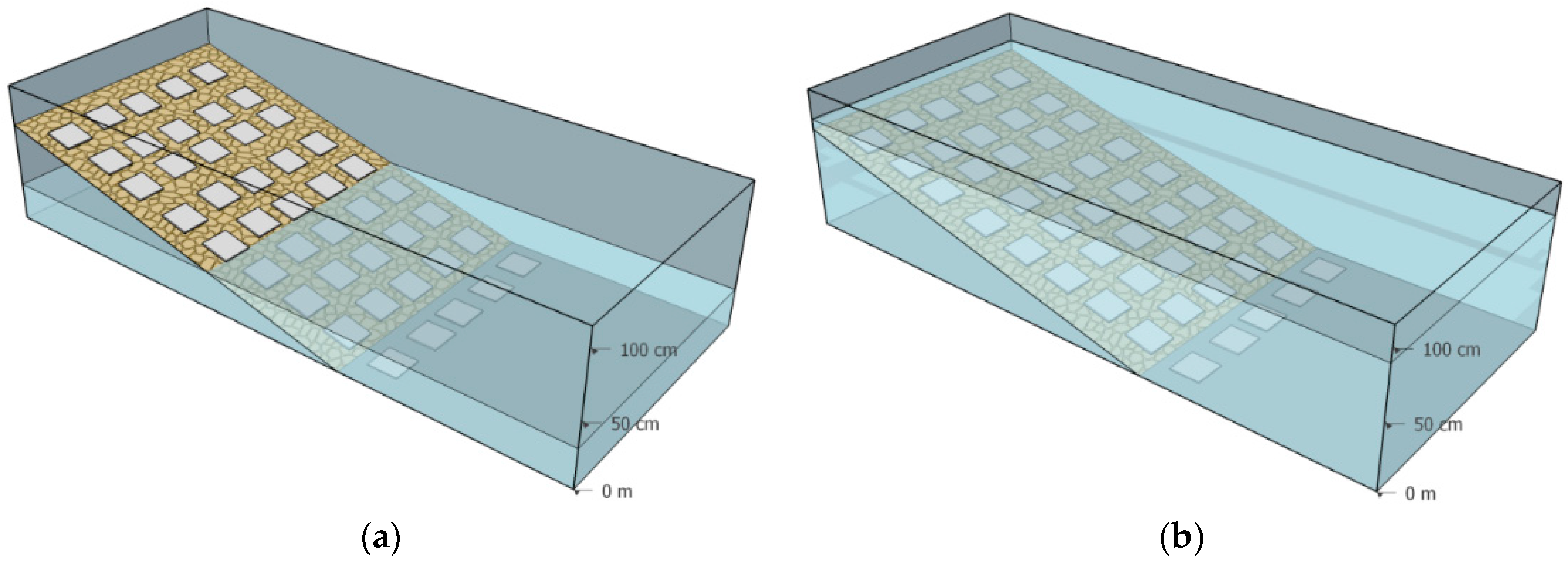
2.1. Experimental Design

We designed an experiment under semi-natural conditions to quantify the effects of WLF on the reservoir ecosystem function. As a proxy for ecosystem function, we used the biomass of benthic algae [15,23]. Because benthic algae provide basic food web energy, we use them as a response variable for environmental effects [24,25].

The experiment was conducted at the Limnological Institute in Constance, Germany, in two outdoor mesocosms (10 × 1 × 1 m dimensions; Figure 1). One mesocosm had a stable water level and served as the control; the other mesocosm served as the treatment (treatment mesocosm). To approximate realistic WLF as the treatment, we applied fluctuations that were previously found to be the most common in terms of frequency and amplitude in alpine reservoirs in the Swiss Alps [5]: a 12 h period of emptying and filling, respectively; with an amplitude of 40 cm corresponding to half the filling level of 80 cm. White square ceramic tiles (10 cm by 10 cm) were used as a standardized substrate because of the unified, easy-to-sample area, homogenous albedo and uniform angle towards the water surface [26]. Five tiles were placed in rows each 10 cm from the water surface (45 tiles × 2 mesocosms). The tiles in the treatment mesocosm at a higher littoral level and experienced longer drying periods than levels further down (see the Results section below). To quantify the loss of benthic algae during the times the littoral areas fall dry, we can relate the amount of time in hours that the levels of tiles fall dry with the loss in benthic algal biomass relative to the inundated control.

To quantify how benthic algae regrow after WLF result in a rise of water level and, thus, a wet fallen surface, we sampled extra tiles for 4 weeks during the growth of the algae prior to the beginning of the WLF experiment. The tiles introduced into the newly-prepared and filled control mesocosm represented newly-inundated reservoir littoral. The experimental timeframe for measuring growth of inundated littoral followed previous estimates from colonization experiments, which have shown that a plateau in algal community development was reached after three weeks [26]. Consequently, the experimental period of 5 weeks ensured that we observed the loss of a natural benthic algal community.

Water exchange rates in both mesocosms were kept constant by applying a flow through of lake water, and a heating system was installed in each mesocosm to unify temperatures. To further ensure standardized growth conditions for periphyton, we measured nutrients (total phosphate and nitrate), temperature (using Hobo^® electronic temperature loggers, Onset, Cape Cod, MA, USA) and light availability (photometer LI-COR, Inc., Lincoln, NE, USA) and analyzed phytoplankton density (estimated from Chl a concentration, see below) as a possible competitor for periphyton for light and nutrients.

2.2. Chlorophyll a Determination: Quantifying Losses to Ecosystem Function via Periphyton Biomass

Benthic algae are a diverse group of photoautotrophic organisms, but they all share chlorophyll a (Chl a) as their main photosynthetic pigment [27]. Consequently, Chl a concentration is the most robust and commonly-applied measure to estimate benthic algal biomass [27]. For standardized sampling, a specifically-constructed periphyton brush sampler (see [28]) was used to brush off 3.14 cm² of each tile. Immediately after sampling, samples were filtrated onto filters (Whatman GF6, 25 mm), folded and frozen at −20 °C in 15 mL falcon tubes wrapped in aluminium foil. Samples were extracted on 90% acetone using an ultrasound bath (Sonorex, 35 kHz) for 30 min, followed by an 8 h storage before centrifuging at 4000 rpm for 10 min. Photometric measurement was conducted by using Infinite 200 following the standard protocol for the monochromatic method of Lorenzen (1967) as described in [29]. Absorption was measured before and after acidification with 1 N HCL in order to correct for pheopigments. Batches of 5 samples were measured at 750 nm (for blank correction) and 665 nm (for Chl a) in triplicate. Since all test samples showed a pH between 7.5 and 7.8, no buffer was added.

2.3. Seasonal Water Levels in Large and Small Alpine Reservoirs

To explore how energy market changes affect WLF dynamics in Swiss reservoirs, we used available data on types of reservoirs [30]. Using two structural indicators, we differentiated and assigned the Swiss hydropower plants into a representative large and small reservoir category (

Table 1. Main characteristics of generic hydropower plants.

	Large	Small
Ratio inflows to storage capacity	2	3098
Full load hours reservoir (hours)	1348	4
Generation capacity (MW)	133	21
Storage Capacity (million m3)	85	0.1

). The first indicator is the ratio of inflows to storage size. The second is the ratio of storage capacity to turbine capacity, which is expressed as the number of hours the plant could run at full capacity until the storage is emptied. Large reservoirs typically show a low inflow ratio and high full load hours. Hydropower plants belonging to this category are seasonal storage reservoirs. Large and deep reservoirs are filled about twice by natural inflows during a hydrological year. Their production capacity is rather low compared to their total storage volume. The opposite is the case for small reservoirs (Table 1).

In our model, the large and small generic hydropower plants represent different operational strategies relevant to our research questions. For the calculation of the benthic algal biomass, we assume that the full depth of the reservoir is suitable habitat for algal growth. This is a reasonable assumption for the small plant type with ca. a 10 m depth, as water clarity in alpine lakes is typically high and ranges between 12 and 15 m [31,32]. The large reservoirs have an average maximum depth of approximately 90 m. Ecologically, this depth means that the reservoir contains bottoms that are so deep that no benthic algae can grow (deeper than the euphotic zone). For simplicity and to ensure the comparability of the results in our modelling of the effect of WLF, we assume that the total lake bottom is available for algal growth in both large and small reservoirs. This clearly is an ecological simplification. The actual ecological benchmark, in terms of loss of benthic algal biomass, that feeds into the model, however, rests on solid empirical data from the experiment. This ensures the scalability of the experimental data to future case studies where more detailed information on the euphotic zone is available.

Price Modelling

Regarding the electricity prices, historic hourly Swiss day-ahead market prices (Swissix) for 2010 and 2015 were compiled from EPEX Spot (European Power Exchange) [33]. These time points were chosen because 5 years is a reasonable period for, e.g., changes in energy legislation to take effect (4 years being a legislative period). Therefore, we chose 5 years into the future (2020) as a forecast scenario. In Switzerland, the electricity market liberalization commenced in 2009, which is why we chose 2010 as the first time point. For 2020 electricity prices, the Swiss electricity market model ‘Swissmod’ developed by Schlecht and Weigt [34,35] was used to derive a price profile for 2020 considering the European and Swiss energy trends. For the price level for 2020, the prices of the Phelix Peak Year Future for 2020 were used [36]. Because we were interested in the effect of changes in the electricity market on the WLF and the algal biomass, we only varied electricity and kept water inflows constant across years [34,35].

2.4. Model Design

The model developed here is based on Hirsch et al. [5] in which the economic operation of a hydropower plant is described within the hydrological system boundaries of the reservoir. The model consists of two parts. In the first part, the hydropower plant is operated according to market prices leading to WLF that follow optimal operation for energy production; in the second part, the WLF are translated into according changes in algal biomass resulting from the economic operation of the reservoir.

2.4.1. Economic Hydropower Operation

The hydropower plant operator maximizes its revenue $R$, which is given by the sum of the hourly spot market prices $p_t$ and the generation $G_t$ over a hydrological year.

$$\text{max}R={\displaystyle \sum }_t{p}_t{G}_t$$

The hourly generation depends on the efficiency of the turbines $\mathsf{\sigma }$, the water density $\mathsf{\rho }$, the gravity $g$, the head $H_t$ and the discharge through the turbines $Q_t$.

$$G_t=\mathsf{\sigma }\mathsf{\rho }g{H}_t{Q}_t$$

In this paper, the head consists of a constant level capturing the penstock between turbines and the storage lake, which is not affected by the reservoir operation, and the reservoir depth, which varies with the economic operation of the reservoir. The storage balance defines the hourly storage level, given by the storage level of the previous period$S_{t-1}$, the natural water inflows into the reservoir $i_t$, the discharge and the residual water $R_t$.

$$S_t=S_{t-1}+i_t-Q_t-R_t$$

The storage level is constrained by the minimum storage level $s^{\min }$ and the maximum storage level$s^{\max }$. The minimum storage level may be influenced by legal constraints.

$$s^{\min }\le S_t\le s^{\max }$$

The hourly discharge is bound by the maximum amount, which can be released through the turbines $q^{\max }$ and the minimum discharge $q^{\min }$.

$$q^{\min }\le Q_t\le q^{\max }$$

The residual water refers to legal obligations $r^{\min }$, which have to be considered in the operation of the reservoirs in Switzerland (see Hirsch et al. [5] for details).

$$R_t\ge r^{\min }$$

The model is formulated as a bi-level formulation in GAMS 23.9. First, a version with constant head level is coded as linear program (LP) and solved by Cplex 12.4. The results are then used as starting point for a version with variable head coded as a non-linear program (NLP) and solved with Conopt3 3.15G.

2.4.2. Quantification of WLF

The basin morphometry influences the extent that littoral zone that falls dry for each unit of water level change. Previous research has found that alpine reservoirs’ basin morphometries are accurately described by a simplified shape of a diagonally-cut pyramid [37]. To translate the changes in the reservoirs’ storage levels we used a mathematical relationship between the storage volume level and the water depth, which we term the depth-volume relationship [38]. This relationship depends on the reservoir’s depth, its volume and the basin morphometry [39] and is given by:

$$S_t=k\times D_t^{\alpha }$$

where $S_t$ is the stored volume level of the reservoir at hour $t$ received from the storage balance equation, $D_t$ the water depth of the reservoir at time point $t$ and $k$ a constant based on the relationship between depth and volume, which is dependent on the reservoir. The more open and flatter the basin, the larger is $k$ [40,41]. The value$\alpha$ defines the concavity of the basin (for further details, see [38,41]). It is important to note here that other morphometries of basins can be specifically addressed using a different reservoir basin equation, which was excluded here for brevity (see [38] for examples). In a similar fashion, the relationship between the storage volume and the corresponding surface area can be calculated by:

$$S_t=c\times A_t^{\alpha }$$

where $A_t$ is the surface area corresponding to a specific storage volume in hour $t$ and $c$ is a constant based on the relationship between the storage volume and the area and the underlying shape of the reservoir.

2.4.3. Translating WLF into Effects on the Ecosystem Function

We used the experimental data to construct a relationship between the time period of inundation or beaching of the littoral surface area and gain or loss in ecosystem function. For each hour, the reservoir has a specific water level resulting from the economic operation of the plant. Assuming depth intervals of 1 m, we defined if a specific depth interval is under water or not at a specific hour. Making use of the depth-volume relationship and the area-volume relationship, the corresponding area for each depth interval could be calculated. Thus, if a depth interval is under water at a specific hour, the corresponding area falls wet. If a depth interval is not under water, the corresponding area falls dry. Based on the experiment, it is assumed that if a specific area falls dry for a certain period of time (see the results below), then there is a complete loss of benthic algae. If a specific area falls wet, we assume the growth of benthic algae that we observed in the experiment as the rate of recovery of ecosystem function. Based on the experimental data on algal biomass per surface area, we can estimate an overall biomass of benthic algae. Thus, we are able to calculate the loss in ecosystem function in % of Chl a relative to a stable water level at which no loss would occur.

2.5. Statistics

When testing for differences in Chl a between treatment and control, we used a hierarchically-nested ANOVA design. This allowed accounting for the fact that tiles at different depths within a mesocosm were not fully independent replicates. Tiles (1–5 for each depth interval) were nested within depth intervals (0–80 depth intervals), and depth intervals were nested within the mesocosm as an overall fixed effect. To test for differences between the scenarios and in ecosystem function (Chl a), we used a generalized linear model with a homogeneity of slopes design, which was found suitable in earlier studies [5]. The test for homogeneity of slopes is related to an ANCOVA, but it does not assume variance homogeneity across factors and can be used to test whether continuous predictors (time in our case) have different effects at different levels of categorical predictors (three one-year scenarios in our case). Because we were only interested in the degree of price variation across yearly scenarios (peek-to-peak spread), we used a simple nested ANOVA for comparing the modelled price developments across scenarios. Hourly prices were nested within months and months within years. More specific information of seasonal price developments are discussed in detail elsewhere [34,35].

3. Results

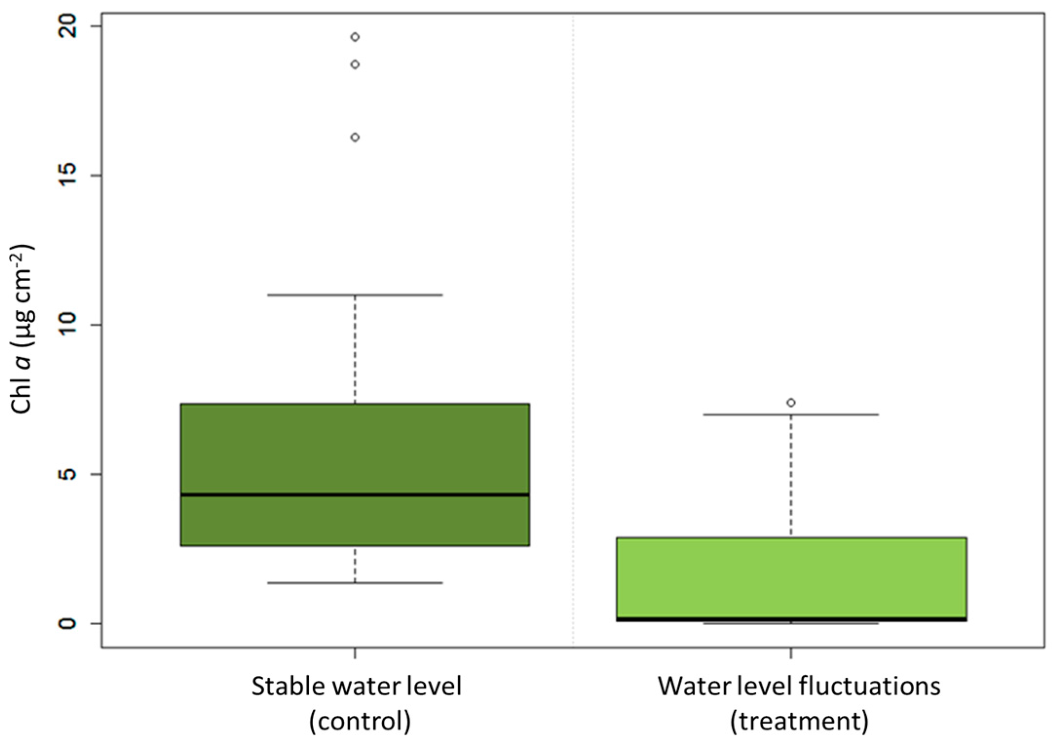
3.1. Experimental Results

WLF significantly decreased ecosystem function, approximated as benthic algal biomass, compared to the mesocosm with stable water levels (nested ANOVA, mesocosm as the fixed effect; df = 1, MS = 397.75, F = 60.33, p < 0.001; Figure 2). In the control mesocosm, Chl a concentration varied from 1.4 µg·cm⁻²–19.7 µg·cm⁻² and in in the treatment WLF-mesocosm from 0 µg·cm⁻²–7.4 µg·cm⁻². The concentration of Chl a did not differ significantly among the tiles used at each depth interval (nested ANOVA, tiles as the random effect; df = 4, MS = 1.73, F = 0.26, p = 0.901).

The overall comparison after five weeks of WLF showed a 74% difference of benthic algal biomass between the mesocosms. The upper littoral zone (80–40 cm above the ground) showed an almost complete loss of 96%, whereas the lower littoral zone (30–0 cm above the ground) showed only partial losses of 61%.

The time dependence of the loss of benthic algae could be inferred by comparing the different levels of tiles and, thus, the time they were dry fallen. The data showed that it takes only 12 h of drought for an almost complete loss of Chl a (

Table 2. Loss in algal biomass measured as Chl a concentration loss for specific durations of WLF relative to the Chl a concentration of the control with stable water levels.

Time Dry Fallen (Hours)	Loss of Chlorophyll a Compared to Wet Fallen Control (%)
20	99.7
18	97.8
14	95.9
12	92.6

). The time dependence of recovery of benthic algae could be inferred by comparing the Chl a concentration from different time periods sampled during the growth of the algae in the pre-experimental period in the mesocosm. The data show that it takes at least seven days for the algae to start growing again, and after 33 days, the algae have recovered completely (

Table 3. Algal growth measured as Chl a concentration for measurement intervals in % of the total algal concentration observed at the end of the experiment when a growth plateau was reached (following published information on benthic algal growth [26]).

Time Wet Fallen (Days)	Growth of Chlorophyll a Compared to Final Value (%)
7	12
14	19
21	34
28	80
33	100

). From the data of the control mesocosm, we could infer a mean concentration of 5718.63 µg·m⁻² (±4354.05 standard deviation SD) Chl a, which we assumed as the basic level of undisturbed ecosystem function.

Abiotic conditions potentially affecting benthic algae were similar between mesocosms. Nutrient concentrations were comparable between mesocosms. Phosphate concentrations were slightly higher in the control mesocosm (control: 12.67 µg·L⁻¹ (±54.19); treatment: 10.10 µg·L⁻¹ (±32.34)), than in the treatment mesocosms, whereas nitrate concentrations showed the opposite pattern and were higher in the treatment than in the control mesocosm (treatment: 613.92 µg·L⁻¹ (±1.78), control: 542.91 µg·L⁻¹ (±1.78)). Temperature did not differ substantially between the treatment (21.08 °C ± 1.6, mean of hourly-logged temperature for all five weeks) and the control mesocosm (21.34 °C ± 1.3). Phytoplankton concentrations were similar between the treatment (0.64 µg·L⁻¹ Chl a ± 0.3, n = 9) and the control mesocosm (0.68 µg·L⁻¹ ± 0.4, n = 9). Finally, the light climate, measured as the ratio of light intensity between the surface and the tiles at different depth intervals, was similar across mesocosms (ratio treatment: 0.75 (±1.28); ratio control: 0.74 (±1.28).

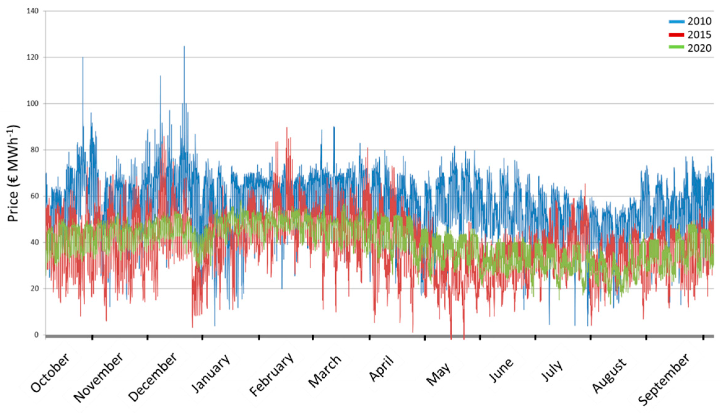
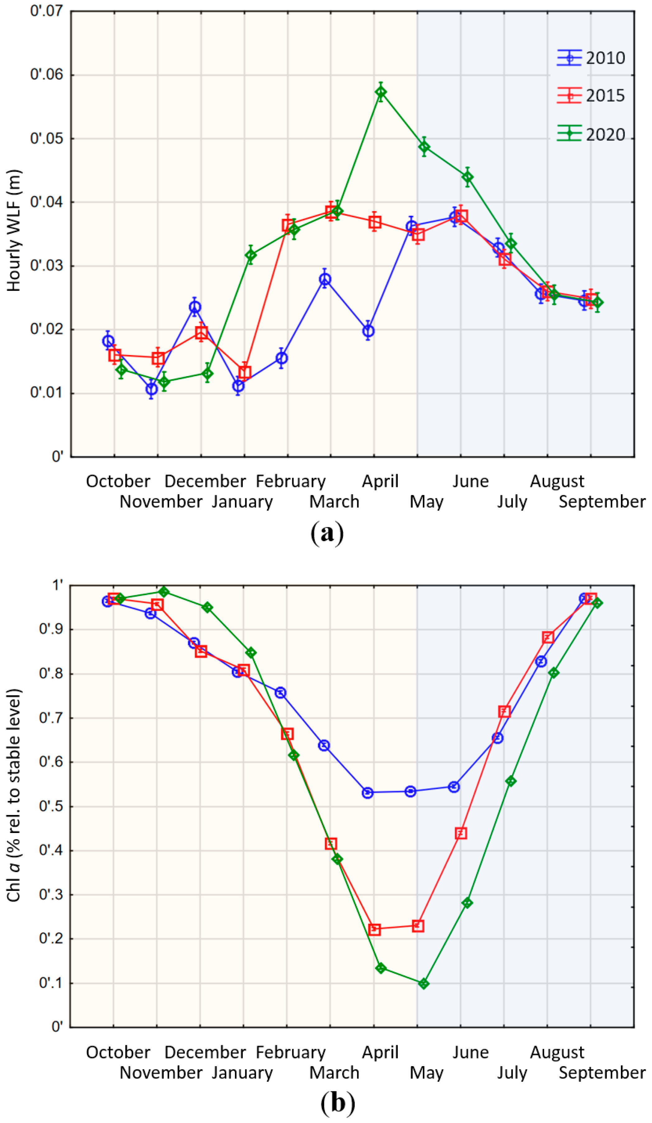
3.2. Modeling Results

The aim of the model simulations was to assess how market changes impact the WLF and thereby the ecosystem function of the storage lake. To capture the different market conditions at different points in time, we first used existing models and data to create the historic hourly price pattern of 2010 and 2015 and the expected price pattern for 2020 (Figure 3). Prices varied across years with 2010 having the highest prices (44.60 €·MWh⁻¹ ± 14.05), whereas the prices in 2015 and 2020 were similar (2015: 38.32 €·MWh⁻¹ ± 13.07; 2020: 39.69 €·MWh⁻¹ ± 12.64). Between the three scenarios, we can observe a significant difference in variance across years (nested ANOVA, df = 2, MS = 827,858.0, F = 49.582, p < 0.001). In concert with the graphical visualization, these differences in variance can be interpreted as differences in price peaks (see Figure 3 for a visualization of peaks and Figure A1 for visualization of the dispersion across years). In the year 2020, price peaks will be much less pronounced than in 2015 and especially compared to 2010. This flattening of peak-to-valley patterns results from increased IRE production, especially solar energy, which reduces the need for conventional supply, thus pushing prices down and reducing price spikes during summer time. Especially the 2020 price curve exhibits a much tighter price range (Figure 3, Figure A1). This is important for hydropower plants, as they aim to maximize production during times of high prices.

3.2.1. Large Reservoirs

In line with our expectation that large reservoirs will adjust operation schemes to changing price dynamics, we find that the different price patterns lead to significant differences in the WLF (homogeneity of slopes test, F = 15.511, df = 2, SS = 0.018, p < 0.001; Figure 4a). However, due to their large storage volume, the mean daily WLF are rather modest with an average of less than 0.1 m (Figure 4a). The years 2015 and 2020 show a much steeper decrease of water levels in the winter months than in 2010, leading to higher average WLF. The 2020 scenario shows the lowest minimum storage level in springtime and consequently has the highest WLF in the late spring and early summer months. This is a result of the low price expectations. Both 2010 and 2015 still show price peaks in May and June (2010) or July (2015) (Figure 3), incentivizing the operator to keep higher storage levels during spring time to benefit from those price levels. For 2020, the WLF follow different economic incentives. The higher winter price levels can be utilized by discharging water rapidly. The resulting lower storage levels in winter can be compensated for by the regular spring and early summer inflows. This provides water to again utilize summer price peaks. The flattening of price peaks in 2020 results in less utilization and consequently less discharge in winter (Figure 4a: October–December). However, the storage of water not utilized in winter is used to utilize price peaks in spring, thus magnifying WLF compared to 2010 and 2015 (Figure 4a: April–June).

The changes in WLF also translate into the benthic algal biomass levels, which differed significantly among the three scenarios (Chl a homogeneity of slopes test, F = 579, df = 2, SS = 0.925, p < 0.001; Figure 4b). Assuming a complete loss of Chl a after 12 h of beaching (Table 2) and a complete re-growth after 33 days of inundation (Table 3), we could quantify the losses and gains of our assumed ecosystem proxy. The seasonality of inflows also dictates the general temporal trend: decreasing areas available for algal growth until spring as the storage lake gets steadily emptied (periods of general filling oremptying storage volumes indicated by shaded areas in Figure 4 and Figure 5), followed by increasing levels in summer months due to increasing water levels. Yet, the three years show differences that are a direct result of operational decisions. The decision to discharge according to pronounced price peaks during spring (March–May) results in a more pronounced loss in ecosystem function in the 2015 and especially in the 2020 scenario (Figure 4b: March–August).

3.2.2. Small Reservoirs

Contrary to large hydropower plants, the differences in the WLF across the three scenarios are not significant in small reservoirs (homogeneity of slopes test, F = 0.23, df = 2, SS = 0.14, p = 0.789; Figure 5). This is in line with our expectation that small plants have less flexibility in adjusting their operation schedules to changing price patterns because the lower inflow ratio precludes longer storage periods. This becomes especially obvious during the late spring and summer months when the inflow level is so high that the storage reservoirs are basically operated like run-of-river plants (Figure 5a: May–August). The WLF during those months is close to zero because all inflows are directly discharged, whilst the storage level is kept close to the maximum. However, the scale of WLF is much higher in the small reservoirs during the fall, winter and spring months (Figure 5a: October–April). This is a result of the ratio between storage and turbine capacity. As indicated in Table 1, it only takes about four hours for such a plant to empty its storage if producing at full capacity. Since the incentive for operation is still price driven, an optimal operation will aim to maximize output in hours with high prices. This leads to a spiked production profile with large discharges in a few hours followed by no production in the following hours until the storage is almost full again. This cycle repeats on a short timeframe leading to pronounced WLF with repetitive wet and dry-fallen littoral zones.

This cycling pattern also translates into the benthic algae biomass (Figure 5b). Albeit that the differences in WLF are insignificant, the effect of WLF on ecosystem function differed significantly among the three scenarios (homogeneity of slopes test, F = 481, degrees of freedom = 2, sum of squares = 1.59, p < 0.001; Figure 5b). This discrepancy between the significances is a result of the dimension of the storage volume. During those months of the year, when the reservoir is operated like a storage reservoir, the daily fluctuations lead to large areas of the lake bottoms beached or inundated in short intervals. In October to April when the reservoir is in a general period of decreasing storage volume, the changes in WLF across scenarios translate into pronounced changes in Chl a. Because small volumetric changes translate into large areas falling dry or wet, the exact timing of a wet-dry cycle of WLF may determine whether a surface area falls dry long enough in one year, but not in the other (Figure 5b). Because it takes 33 days until benthic algae have completely regrown (Table 3), even the small variations in WLF between the scenarios lead to large effects on the ecosystem function. Yet, during the summer months when the plant is operated like a run-of-river plant, the storage has a relatively stable level and consequently is close to the theoretically-possible maximum biomass level (Figure 5b: June–September).

4. Discussion

4.1. Economic Changes Translate into Ecological Changes

In this study, we aimed to combine economic and ecological benchmarks to facilitate a compromise between maximizing profit and ecosystem function based on scientific data. To this end, we quantified ecosystem function as biomass of the basic food web level and modeled scenarios of energy market developments in small and large alpine reservoirs. We demonstrate how WLF affect the ecosystem function of reservoirs across three different annual price scenarios. Our results suggest that changing energy prices due to, e.g., the development of IRE affect hydropower operations, WLF and, eventually, ecosystem function. Importantly, we found that small and large reservoirs respond differently, and effects vary in their seasonality across the calculated scenarios. This demonstrates the need for research that appreciates the specific differences of hydropower plants. Research on sustainable hydropower reservoir development has long acknowledged the need for quantifying and combining economic benchmarks with ecological benchmarks. For example, informed compromises based on cooperatively-achieved and discussed research results can consolidate economic, environmental and social aspects in the decision to flood valleys for creating reservoirs [42,43]. Advances have recently been made in the mathematical modelling of hydropower flow regimes that consider both economic benchmarks and ecological benchmarks. The concept of environmental flows allows one to quantify ecological water demands downstream of hydropower dams [8]. Which flows are required is based on research that appreciates the ecological needs of the respective ecosystem [44]. Our study advances these previous finding by focussing on the environmental effects of hydropower also within the reservoir itself and by accounting for dynamics in economic processes that influence reservoir operation. Our results suggest that both economic and ecological benchmarks should be considered differently in small and large reservoirs. The available storage volume determines how the reservoir’s operation translates into WLF and, eventually, ecosystem functions. In smaller reservoirs, the operation during winter months results in much more pronounced WLF and, hence, changes in ecosystem function, because responses to price changes are more directly reflected in lake bottom areas that fall wet or dry. Research on environmental flows has put forward models that can create mathematical compromises for possibly conflicting water demands [45]. Accordingly, our results can form the basis for such a quantification of economic and environmental demands also for reservoirs, thus providing a knowledge basis for communication amongst decision makers.

4.2. Implications and Context of Experimental Results

Several fundamental ecosystem processes are affected when WLF cause changes in the littoral zone from the aqueous phase to the dry phase. We used empirically-validated effects of WLF on benthic algae as a proxy for further ecosystem effects of WLF. Clearly, there are more complicated indirect effects from WLF than decreases in benthic algae biomass. However, benthic algae are such an essential component of freshwater ecosystem function that they are a major environmental variable commonly applied as indicator organisms for total ecosystem health [46]. For example, the monitoring of benthic algae can help to establish causative effects of stressors, such as WLF, and periphyton-based ecosystem assessment is considered a powerful tool to quantify the ecological status of lakes [47]. Furthermore, research shows that losses of benthic primary production can cascade up to higher food web levels, altering trophic relationships at higher levels of the food chain [23]. Especially nutrient poor, clear and montane lakes react sensitively to changes in the benthic algal biomass [48]. Montane lakes, such as Lake Constance, where we conducted our experiments, can have food webs that rely on undisturbed lake bottoms and shoreline areas, not only for benthic algae, but also for, e.g., spawning and nursing grounds of fish [49]. Due to their role of storing and balancing IRE, most reservoirs will be developed in mountainous areas where the topography allows for storing water at higher heads [5]. This would mean that the development of hydropower to balance IRE will occur in ecosystems that are especially sensitive to the possible environmental effects caused by WLF. The high sensitivity of benthic algae to changes in WLF is highlighted by our model data from small reservoirs. Despite WLF being not significantly different across the three yearly scenarios (2010, 2015, 2020), we detected a significant change in benthic algae biomass in small reservoirs.

4.3. Implications and Context of Modeling Results

The model results indicate that hydropower plant operation and its effect on the reservoir ecosystem function are sensitive to market changes. The simulations show that the ecological effects differ substantially depending on scenario and that small changes in the economic conditions can have significant influences on the ecosystem function. For large hydropower plants variations in prices, but also available water storage are the main drivers that will influence the algal biomass levels over the year. For small hydropower plants, the limited storage volume dictates a more volatile operational schedule. On the one hand, this translates into a lower impact of market prices on the yearly production pattern. On the other hand, this entails a more direct effect of small operational deviations on ecological benchmarks. In total, the results for 2015 and 2020 show a lower Chl a level than the 2010 scenario. This is likely a result of the increase in IRE generation that leads to lower price levels and a reduced spread between peak and off-peak prices. Given that many European electricity markets are in a transition towards a higher share of IRE, the simulated impacts may further increase in coming decades. However, electricity market prices are also highly sensitive to global fuel price developments, carbon prices, further policy decisions and, in the case of small countries like Switzerland, also to the developments of neighboring countries [50,51]. Our model only varied price levels, but kept the seasonal inflow pattern constant over the years. Against this background, it is particularly striking that our models detected changes in the seasonality of WLF. The effect of market changes on the seasonality of WLF can have ramifications for ecosystem responses to the energy transition to IRE that are presently underappreciated.

4.4. Transferability and Future Advancements Based on Experimental Results

Our experiments were conducted under conditions that approximate those of alpine reservoirs. By definition, Lake Constance also is an alpine lake because it is located in a montane zone. The lake’s nutrient concentrations match those of alpine lakes. For example, the nutrient phosphorous, which is used as a proxy to describe the overall productivity of an aquatic ecosystem, is approximately 6–7 µg·L⁻¹ in Lake Constance, which corresponds to the level of a naturally nutrient-poor alpine lake. By using water directly from the lake, we could thus create conditions that match those of alpine reservoirs. One crucial aspect that requires further testing is the seasonality of water level changes. Hydropower reservoirs typically follow a seasonal filling and emptying pattern throughout the hydrological year. Due to experimental constraints, data acquisition focused on a relevant, but limited time during summer. In accordance with the implications of our modelling data, future experimental studies should address seasonal changes and, ideally, be conducted over a complete hydrological year. This will also allow a more detailed assessment of ecological effects. Models to account for the effect of climate change on reservoir operation have already demonstrated that inflows, and thus operation, can be affected by climate change [5]. More detailed and parameterized climate models will also improve our knowledge on the ecosystem effects in specific geographic areas.

4.5. Transferability and Future Advancements Based on Modeling Results

In general, our model is applicable to other storage hydropower plants in order to examine similar issues. However, every model has some shortcomings. In our case, the underlying form of the lake is a simplification. Even if it might be accurate for Alpine reservoirs in Switzerland [38,41], it might not be accurate for reservoirs in other geographic regions. In addition, the change in the Chl a concentration for larger depths than 30 m depends on complex relationships between water clarity, photosynthetically-active radiation and the slope of the reservoir basin. These variables include a complexity that we did not address to maintain our results as generic and applicable to a wide range of conditions. When applying our generic models to specific reservoirs as case studies, researchers will have the chance to parameterize such variables accordingly. This will make reservoir-specific models more realistic and thus more applicable also for feeding scientific results into local policy processes. By building our models for generic hydropower plants and reservoirs, our analyses could identify general patterns for alpine areas of Switzerland. In our case, we varied electricity prices over the scenarios, but kept the variations in inflows constant over the three scenario years. This allowed us to distill effects induced by market price changes, albeit with some uncertainty, regarding the electricity prices for 2020. Since the underlying market model is based on assumptions about future developments, the actual prices can develop differently up to 2020. Disentangling the effect of changes in the water inflows and the effect of changes in the electricity prices would require much more elaborate climate modelling capacities, which were not the focus of this study. Uncertainty about future price potentials may induce different operation strategies; i.e., keeping more water within the storage to benefit from expected price increases or releasing more water due to expected price decreases. Future non-deterministic models can help to explore how additional variables influence the developments of economic and thus ecological benchmarks.

4.6. Relevance for the Context of sustainable development and the Achievement of SDG #7

Our analysis sheds light on the complexity of sustainable energy provision. While in the global context, hydropower is typically perceived as a carbon-poor and environmentally-friendly source of energy, the picture becomes less clear on a local scale. The aspect of WLF and the ecosystem functions of storage reservoirs adds to the already challenging task of consolidating the development of hydropower with the preservation of affected ecosystems. Recent research emphasizes the need to balance the economic gains from hydropower generated by dams in running rivers with the negative ecological effects on, e.g., migratory fish species [52]. This case presents a trade-off between global benefits in the form of low-carbon energy and local costs in the form of potential harmful ecological effects. In addition to biomass production of benthic algae as a proxy, we have to consider further ecosystem functions, such as linkage with terrestrial ecosystems and also recreational issues, which can be influenced by the aesthetic effects of WLF [53].

Aiming to represent real-world conditions, our modeling was based on the assumption that reservoir operation rests purely on the incentive of profit maximization. By describing the WLF effect on ecosystem function, our approach allows defining ecological boundary conditions to maintain ecosystem functions, such as minimum time periods of stable water level. Using our generic model, we can then quantify the economic costs in the form of foregone profits for a specific reservoir in which such ecological boundary conditions would be installed. As has been shown in the case of the small reservoir category already, small operational changes could have profound effects on the biomass levels. A small correction is likely to have only a small impact on the obtainable profit, but can provide benefits for the function of the ecosystem. The approach presented here bridges the two major pillars of sustainable development. Considering environmental effects, but also accounting for economic sustainability (in the form of sufficient revenue streams for the operator) is a crucial step for the knowledge building process towards sustainable development [2].

5. Conclusions and Outlook

Few studies have considered how hydropower operations affect ecological processes within the actual reservoir itself. This is a gap of knowledge because reservoirs provide important ecosystem functions beyond energy production. Some of these functions have recently been recognized as relevant in the context of WLF and are promising avenues of future research in this direction. For example, lake and reservoir sediments bury more carbon annually than oceanic carbon sinks, and topical research suggests that drastic WLF can affect the carbon burial, hence altering the role of reservoirs in the global carbon cycle [54,55]. Against the background of reservoirs providing not only energy, but also ecosystem services, sustainable development needs to acknowledge that both cannot be maximized. The future aim will thus be to balance the ecosystem function of reservoirs with energy production. The role of hydropower in facilitating the transition towards low-carbon energy supply and the potential effects of reservoirs in the global carbon cycle should be a topic for further study. Our results demonstrate the potential to combine economic and ecological benchmarks to provide scientific data for further decision making. Ideally, to acknowledge all three pillars of sustainable development, our study should instigate research into the societal aspects of the Sustainable Development Goal #7. For example, restrictions on the frequency or amplitude of WLF can be introduced to protect a desirable level of ecosystem function. These restrictions need not only be based on scientific evidence, but also be communicated with relevant players of the social domain, such as decision makers (i.e., the operators of hydropower reservoirs) and the general public. Such a process should follow guidelines for research with and for society [56]. The attainment of the SDG, especially of Goal #7, calls for such action, but any process towards sensible policies must rely on solid scientific contributions. Studies addressing not only all three pillars of sustainable development, but also their future development will greatly advance researchers’ ability to contribute with scientific analysis to the sustainable development of hydropower.

References

1. United Nations. Transforming Our World: The 2030 Agenda for Sustainable Development—Outcome Document of Summit for Adoption of the Post-2015 Development Agenda; United Nations: New York, NY, USA, 1996; Volume A/RES/70/1. [Google Scholar]
2. Clark, W.C.; van Kerkhoff, L.; Lebel, L.; Gallopin, G.C. Crafting usable knowledge for sustainable development. Proc. Natl. Acad. Sci. USA 2016, 113, 4570–4578. [Google Scholar] [CrossRef] [PubMed]
3. Kumar, A.; Schei, T.; Ahenkorah, A.; Caceres Rodriguez, R.; Devernay, J.-M.; Freitas, M.; Hall, D.; Killingtveit, Å.; Liu, Z. Hydropower; Cambridge University Press: Cambridge, UK, 2011. [Google Scholar]
4. Friedl, G.; Wüest, J. Fresh Water Volume III—Human-Made Lakes and Reservoirs: The Impact of Physical Alterations. Encyclopedia of Life Support Systems (EOLSS), Developed under the Auspices of the UNESCO; Eolss Publishers: Paris, France, 2016. [Google Scholar]
5. Hirsch, P.E.; Schillinger, S.; Weigt, H.; Burkhardt-Holm, P. A hydro-economic model for water level fluctuations: Combining limnology with economics for sustainable development of hydropower. PLoS ONE 2014, 9, e114889. [Google Scholar] [CrossRef] [PubMed]
6. Collen, B.; Whitton, F.; Dyer, E.E.; Baillie, J.E.M.; Cumberlidge, N.; Darwall, W.R.T.; Pollock, C.; Richman, N.I.; Soulsby, A.-M.; Böhm, M. Global patterns of freshwater species diversity, threat and endemism. Glob. Ecol. Biogeogr. 2014, 23, 40–51. [Google Scholar] [CrossRef] [PubMed]
7. García Molinos, J.; Viana, M.; Brennan, M.; Donohue, I. Importance of long-term cycles for predicting water level dynamics in natural lakes. PLoS ONE 2015, 10, e0119253. [Google Scholar] [CrossRef] [PubMed]
8. Poff, N.L.; Matthews, J.H. Environmental flows in the anthropocence: Past progress and future prospects. Curr. Opin. Environ. Sustain. 2013, 5, 1–9. [Google Scholar] [CrossRef]
9. Duan, W.X.; Guo, S.L.; Wang, J.; Liu, D.D. Impact of cascaded reservoirs group on flow regime in the middle and lower reaches of the yangtze river. Water 2016, 8, 218. [Google Scholar] [CrossRef]
10. Hirsch, P.; Eloranta, A.; Amundsen, P.-A.; Brabrand, Å.; Charmasson, J.; Helland, I.; Power, M.; Sánchez-Hernández, J.; Sandlund, O.; Sauterleute, J.; et al. Effects of anthropogenic water level fluctuations in reservoirs—An ecosystem approach with a special emphasis on fish. Hydrobiologia 2016. submitted. [Google Scholar]
11. Evtimova, V.; Donohue, I. Quantifying ecological responses to amplified water level fluctuations in standing waters: An experimental approach. J. Appl. Ecol. 2014, 51, 1282–1291. [Google Scholar] [CrossRef]
12. Moss, B. The kingdom of the shore: Achievement of good ecological potential in reservoirs. Freshw. Rev. 2008, 1, 29–42. [Google Scholar] [CrossRef]
13. Dieter, D.; Herzog, C.; Hupfer, M. Effects of drying on phosphorus uptake in re-flooded lake sediments. Environ. Sci. Pollut. Res. 2015, 22, 17065–17081. [Google Scholar] [CrossRef] [PubMed]
14. Weise, L.; Ulrich, A.; Moreano, M.; Gessler, A.; Kayler, Z.E.; Steger, K.; Zeller, B.; Rudolph, K.; Knezevic-Jaric, J.; Premke, K. Water level changes affect carbon turnover and microbial community composition in lake sediments. FEMS Microbiol. Ecol. 2016, 92, fiw035. [Google Scholar] [CrossRef] [PubMed]
15. Vadeboncoeur, Y.; Vander Zanden, M.J.; Lodge, D.M. Putting the lake back together: Reintegrating benthic pathways into lake food web models. Bioscience 2002, 52, 44–54. [Google Scholar] [CrossRef]
16. Hampton, S.E.; Fradkin, S.C.; Leavitt, P.R.; Rosenberger, E.E. Disproportionate importance of nearshore habitat for the food web of a deep oligotrophic lake. Mar. Freshw. Res. 2011, 62, 350–358. [Google Scholar] [CrossRef]
17. Yang, Y.; Yin, X.A.; Chen, H.; Yang, Z.F. Determining water level management strategies for lake protection at the ecosystem level. Hydrobiologia 2014, 738, 111–127. [Google Scholar] [CrossRef]
18. Yang, N.; Mei, Y.; Zhou, C. An optimal reservoir operation model based on ecological requirement and its effect on electricity generation. Water Resour. Manag. 2012, 26, 4019–4028. [Google Scholar] [CrossRef]
19. Wang, Y.Y.; Jia, Y.F.; Guan, L.; Lu, C.; Lei, G.C.; Wen, L.; Liu, G.H. Optimising hydrological conditions to sustain wintering waterbird populations in poyang lake national natural reserve: Implications for dam operations. Freshw. Biol. 2013, 58, 2366–2379. [Google Scholar] [CrossRef]
20. Barry, M.; Baur, P.; Gaudard, L.; Giuliani, G.; Hediger, W.; Romerio, F.; Schillinger, M.; Schumann, R.; Voegeli, G.; Weigt, H. The Future of Swiss Hydropower—A Review on Drivers and Uncertainties; FoNEW Discussion Paper 2015/01; Social Science Research Network (SSRN): Rochester, NY, USA, 2015. [Google Scholar]
21. N’Guyen, A.; Hirsch, P.E.; Adrian-Kalchhauser, I.; Burkhardt-Holm, P. Improving invasive species management by integrating priorities and contributions of scientists and decision makers. Ambio 2016, 45, 280–289. [Google Scholar] [CrossRef] [PubMed]
22. Hirsch, P.E.; Adrian-Kalchhauser, I.; Flaemig, S.; N’Guyen, A.; Defila, R.; di Giulio, A.; Burkhardt-Holm, P. A tough egg to crack: Recreational boats as vectors for invasive goby eggs and transdisciplinary management approaches. Ecol. Evol. 2016, 6, 707–715. [Google Scholar] [CrossRef] [PubMed]
23. Vander Zanden, M.J.; Vadeboncoeur, Y.; Chandra, S. Fish reliance on littoral-benthic resources and the distribution of primary production in lakes. Ecosystems 2011, 14, 894–903. [Google Scholar] [CrossRef]
24. Coops, H.; Beklioglu, M.; Crisman, T.L. The role of water-level fluctuations in shallow lake ecosystems—Workshop conclusions. Hydrobiologia 2003, 506, 23–27. [Google Scholar] [CrossRef]
25. Zohary, T.; Ostrovsky, I. Ecological impacts of excessive water level fluctuations in stratified freshwater lakes. Inland Waters 2011, 1, 47–59. [Google Scholar] [CrossRef]
26. Peters, L.; Wetzel, M.A.; Traunspurger, W.; Rothhaupt, K.-O. Epilithic communities in a lake littoral zone: The role of water-column transport and habitat development for dispersal and colonization of meiofauna. J. N. Am. Benthol. Soc. 2007, 26, 232–243. [Google Scholar] [CrossRef]
27. Azim, M.E.; Verdegem, M.C.J.; van Dam, A.A.; Beveridge, M.C.M. Periphyton: Ecology, Exploitation, and Management; CABI Publishing: Wallingford, UK; Cambridge, MA, USA, 2005. [Google Scholar]
28. Peters, L.; Scheifhacken, N.; Kahlert, M.; Rothhaupt, K.O. An efficient in situ method for sampling periphyton in lakes and streams. Arch. Hydrobiol. 2005, 163, 133–141. [Google Scholar] [CrossRef]
29. Wetzel, R.G.; Likens, G.E. Limnological Analyses; Springer: Berlin, Germany, 1991; p. 391. [Google Scholar]
30. Balmer, M. Nachhaltigkeitsbezogene Typologisierung der Schweizerischen Wasserkraftanlagen. Gis-Basierte Clusteranalyse und Anwendung in Einem Erfahrungskurvenmodell. Ph.D. Thesis, Department of Mechanical and Process Engineering ETH Zürich, Zürich, Switzerland, 2012. [Google Scholar]
31. James, G.D.; Graynoth, E. Influence of fluctuating lake levels and water clarity on trout populations in littoral zones of new zealand alpine lakes. N. Z. J. Mar. Freshw. Res. 2002, 36, 39–52. [Google Scholar] [CrossRef]
32. Hutter, K.; Chubarenko, I.P.; Wang, Y. Physics of Lakes: Volume 3: Methods of Understanding Lakes as Components of the Geophysical Environment; Springer: Berlin, Germany, 2014. [Google Scholar]
33. EPEXSPOT. Marktdaten Day-Ahead-Auktion. Available online: https://www.Epexspot.Com/de/marktdaten (accessed on 25 May 2016).
34. Schlecht, I.; Weigt, H. Linking europe—The role of the swiss electricity transmission grid until 2050. Swiss J. Econ. Stat. 2015, 151, 39–79. [Google Scholar] [CrossRef]
35. Schlecht, I.; Weigt, H. Swissmod—A Model of the Swiss Electricity Market; WWZ Discussion Paper 2014/04; IDEAS: Ottawa, ON, Canada, 2014. [Google Scholar]
36. EEX. Phelix Power Futures—EEX Power Derivatives. Available online: https://www.Eex.Com/en/market-data/power/futures/phelix-futures#!/2016/06/02 (accessed on 25 May 2016).
37. Finger, D.; Heinrich, G.; Gobiet, A.; Bauder, A. Projections of future water resources and their uncertainty in a glacierized catchment in the swiss alps and the subsequent effects on hydropower production during the 21st Century. Water Resour. Res. 2012, 48. [Google Scholar] [CrossRef]
38. Liebe, J.; van de Giesen, N.; Andreini, M. Estimation of small reservoir storage capacities in a semi-arid environment—A case study in the upper east region of Ghana. Phys. Chem. Earth 2005, 30, 448–454. [Google Scholar] [CrossRef]
39. Shang, S. Lake surface area method to define minimum ecological lake level from level-area-storage curves. J. Arid Land 2013, 5, 133–142. [Google Scholar] [CrossRef]
40. Kühne, A. Charakteristische Kenngrössen schweizer Speicherseen. Geogr. Helv. 1978, 33, 191–199. [Google Scholar] [CrossRef]
41. Rodrigues, L.; Liebe, J. Small reservoirs depth-area-volume relationships in savannah regions of Brazil and Ghana. Water Resour. Irrig. Manag. 2013, 1, 1–10. [Google Scholar]
42. Opricovic, S. A compromise solution in water resources planning. Water Resour. Manag. 2008, 23, 1549–1561. [Google Scholar] [CrossRef]
43. Stevovic, S.; Milovanovic, Z.; Stamatovic, M. Sustainable model of hydro power development—Drina river case study. Renew. Sustain. Energy Rev. 2015, 50, 363–371. [Google Scholar] [CrossRef]
44. Jager, H.I.; Smith, B.T. Sustainable reservoir operation: Can we generate hydropower and preserve ecosystem values? River Res. Appl. 2008, 24, 340–352. [Google Scholar] [CrossRef]
45. Shiau, J.-T.; Chou, H.-Y. Basin-scale optimal trade-off between human and environmental water requirements in hsintien creek basin, taiwan. Environ. Earth Sci. 2016, 75, 644. [Google Scholar] [CrossRef]
46. Omar, W.M.W. Perspectives on the use of algae as biological indicators for monitoring and protecting aquatic environments, with special reference to malaysian freshwater ecosystems. Trop. Life Sci. Res. 2010, 21, 51–67. [Google Scholar] [PubMed]
47. DeNicola, D.M.; Kelly, M. Role of periphyton in ecological assessment of lakes. Freshw. Sci. 2014, 33, 619–638. [Google Scholar] [CrossRef]
48. Karlsson, J.; Byström, P.; Ask, J.; Ask, P.; Persson, L.; Jansson, M. Light limitation of nutrient-poor lake ecosystems. Nature 2009, 460, U506–U580. [Google Scholar] [CrossRef] [PubMed]
49. Stoll, S. Complex interactions between pre-spawning water level increase, trophic state and spawning stock biomass determine year-class strength in a shallow-water-spawning fish. J. Appl. Ichthyol. 2013, 29, 617–622. [Google Scholar] [CrossRef]
50. Swiss Federal Office of the Environment. Swiss Electricity Statistic; SFOE: Bern, Switzerland, 2014.
51. Swiss Federal Office of the Environment. Swiss Electricity Statistic; SFOE: Bern, Switzerland, 2010.
52. Nieminen, E.; Hyytiäinen, K.; Lindroos, M. Economic and policy considerations regarding hydropower and migratory fish. Fish Fish. 2016. [Google Scholar] [CrossRef]
53. Schramm, M.P.; Bevelhimer, M.S.; DeRolph, C.R. A synthesis of environmental and recreational mitigation requirements at hydropower projects in the United States. Environ. Sci. Policy 2016, 61, 87–96. [Google Scholar] [CrossRef]
54. López, P.; López-Tarazón, J.A.; Casas-Ruiz, J.P.; Pompeo, M.; Ordoñez, J.; Muñoz, I. Sediment size distribution and composition in a reservoir affected by severe water level fluctuations. Sci. Total Environ. 2016, 540, 158–167. [Google Scholar] [CrossRef] [PubMed]
55. Gudasz, C.; Bastviken, D.; Steger, K.; Premke, K.; Sobek, S.; Tranvik, L.J. Temperature-controlled organic carbon mineralization in lake sediments. Nature 2010, 466, 478–481. [Google Scholar] [CrossRef] [PubMed]
56. Seidl, R.; Brand, F.S.; Stauffacher, M.; Kruetli, P.; Le, Q.B.; Spoerri, A.; Meylan, G.; Moser, C.; Gonzalez, M.B.; Scholz, R.W. Science with society in the Anthropocene. Ambio 2013, 42, 5–12. [Google Scholar] [CrossRef] [PubMed]
Figure 1. Schematic illustration of the experimental setup. Tiles were aligned in rows at a 10 cm height difference, whereby one row forms a littoral level. (a) The minimum water level was 40 cm above the ground; (b) The maximum water level was at 80 cm above the ground.
Sustainability 08 00875 g001
Figure 2. Chlorophyll a concentration in the control mesocosm with stable water level (control) was higher than in the treatment mesocosm in which water level fluctuations (WLF) caused substrates to fall dry (treatment).
Sustainability 08 00875 g002
Figure 3. Development of electricity prices in € per MWh as modelled for the three scenarios 2010 (blue line), 2015 (red line) and 2020 (green line). Based on [33,34,35]. See Figure A1 for bagplots of year scenarios.
Sustainability 08 00875 g003
Figure 4. Modelled changes of water level regime and ecosystem function in large Swiss reservoirs. The yellow shaded area marks a period of high inflows into the reservoir, whereas the blue shaded area marks a period of no or little inflows. (a) Development of WLF in Swiss alpine reservoirs in the context of different energy market developments in three modelled scenarios 2010, 2015 and 2020. WLF are expressed as absolute changes (including increases and decreases of water level) per hour (Appendix Figure A2 shows WLF with algebraic sign); (b) Development of ecosystem function in Swiss alpine reservoirs in the context of future energy market development. Ecosystem function is expressed in % Chl a compared to a stable water level. Accordingly, zero means no losses, whereas 0.1 means a loss of 10% compared to a stable water level. Different colors and symbols denote the three different scenarios (2010 green diamonds, 2015 red squares, 2020 blue circles).
Sustainability 08 00875 g004
Figure 5. Modelled changes of water level regime and ecosystem function in small Swiss reservoirs (a) Development of WLF in small Swiss alpine reservoirs in the context of different energy market developments in three modelled scenarios 2010, 2015 and 2020. The yellow shaded area marks a period of high inflows into the reservoir, whereas the blue shaded area marks a period of no or little inflows. WLF are expressed as absolute changes (including increases and decreases of water level) per hour (Appendix Figure A2 shows WLF with algebraic sign); (b) Development of ecosystem function in Swiss alpine reservoirs in the context of future energy market development. Ecosystem function is expressed in % Chl a compared to a stable water level. Accordingly, zero means no losses, whereas 0.1 means a loss of 10% compared to a stable water level. Different colors and symbols denote the three different scenarios (2010 green diamonds, 2015 red squares, 2020 blue circles).
Sustainability 08 00875 g005