1. Introduction
Oklahoma possesses some of the best wind resources in the world. However, wind regimes are dynamic in nature. They are fickle over scales of seconds, minutes, years and decades. Over long time periods, the characteristics of wind (strength, direction and variability) are sensitive to climate changes. This study focuses on how climate change could impact future wind resources in western Oklahoma, with attention to a gain or loss in resulting power generation.
A fundamental concern with all renewable energy based on meteorological parameters is determining the variability and reliability of that resource on various spatial and temporal scales [
1]. In terms of electrical generation from wind, a site’s wind resource is the driver of financial income streams, including power production agreements, selling wind energy, receiving renewable energy credits, production tax credits and other sources of revenue. Current data show that the installed cost of 1 megawatt (MW) of wind generation capacity is close to $2,000 [
2]. Therefore, investment into a modest-sized wind farm of 100 MW total capacity can be more than 200 million dollars. It is clear that such investment needs as much informed long-term wind characterization as is possible; huge capital investments in resources are not made lightly.
The Intergovernmental Panel on Climate Change (IPCC) determined through a consensus-based scientific process that human activity is having a significant net warming effect on the globe: “Human interference with the climate system is occurring, and climate change poses risks for human and natural systems” [
3]. Modern wind power development has relied on careful characterization of a potential site’s wind regime, so that turbines can be operated profitably [
4,
5]. Wind information is vital for financing and building multi-million dollar wind farms. The wind industry’s practice is to gather wind measurements from very few tall towers for a few months and to compare them with long-term wind records from (invariably) lower measurement heights at other locations to insure that the tower measurements are in line with the longer-term climatology. However, what happens if today’s regime is not tomorrow’s regime? In a world of climate change, investors are not altogether safe to compute their return on investment using recent wind data.
There is ample evidence from the climatic past and climate modeling of the future that climate change cannot be expected to work in ways that are globally monotonic [
3]. While “warming” is the term assigned to global climate change of the 21st century, outputs of various global climate models using various scales and scenarios demonstrate that other atmospheric parameters are projected to change, as well. When examining numerical outputs of any of the major climate models, it is manifest that wind resource changes will vary regionally.
Pryor
et al. [
6] note that any changes in near-surface wind velocities caused by global climate change could have major societal impacts. From the current authors’ perspective, wind changes are a major concern for places depending on significant amounts of wind generation. For instance, possible wind climate changes are not a trivial concern in Oklahoma. The state now derives approximately 15% of its electrical generation from wind, with greater development slated to occur [
7]. The purpose of the present article is to illustrate regional spatial differences in model output for future Oklahoma wind and to calculate potential future power generation at a pair of wind farms.
1.1. Changes in Historic Winds
Global weather is the result of energy transfer from the Equator to the poles by atmosphere and ocean. Climatological wind changes at individual locations are partially tied to changes in global circulation and so is the resulting energy that can be derived from wind. Research on recent historic change in wind velocities ranges from international to regional scales.
Palutikof
et al. [
8] found a decrease in wind velocity of roughly two meters per second over a sixty-year period in Britain, translating into an 18% decrease in energy output. Other studies concluded that there was a decline in wind speeds across much of the continental United States, resulting in lowering average wind power. Other research noted more than 30% drops in average wind power density in some places [
9,
10]. Brazdil
et al. [
11] identified statistically significant falling mean wind-speed trends for months, seasons and years over the time period of 1961–2005 in the Czech Republic.
Tammelin
et al. [
12] commented on how climate strongly affects the potential power production of renewable energy sources, addressing the effect of climate change on wind power by 2020. Using Hadley Center CO
2 emission scenarios showed that the result would be increased average wind speeds of about 7% over the Nordic region. This overview indicated increased wind speeds in the future, mostly in the winter months [
13].
On a seasonal time scale, winter wind speeds could increase as much as 5% to 10% in northern England and Scotland, with slight decreases possible in the summer months [
14]. Working in the United States, Klink also found significant variation of winds by season [
15,
16].
Many countries have considerable economic interest in the potential impact of climate change on wind resources. If the above trends are short-term anomalies around a long-term stationary mean into the future, this would not be significant. However, it is doubtful that the long-term means will remain stationary considering the corpus of climate change literature [
17]. Therefore, increases and decreases of wind speeds found in the literature cast considerable uncertainty on the investments of these countries in major penetration of wind power in energy generation portfolios.
1.2. Modeling Future Wind
Climatological models have become increasingly adept at producing mesoscale outputs. In our work, we used well-vetted modeled wind outputs from the North American Regional Climate Change Assessment Program (NARCCAP) and applied them to future wind generation using turbine characteristics of actual sites [
18]. This allowed us to examine the impacts of changes in wind velocities on the output of two wind farms.
The methodological consensus in modeling future winds in regional settings is to downscale global climate models (GCMs). Commonly, this is accomplished with various carbon dioxide emission scenarios, such as specified by the IPCC [
17]. To check model accuracy, a reanalysis is run on past climate with the model and compared to wind observations from the same time period. Reanalysis data are compared to prognostic emission scenarios to examine differences [
19].
Reanalysis involves three-dimensional forecasting that is initialized with real climate observations, such as temperature, wind speed and pressure. Reanalysis efforts have been fairly successful, and model runs show general qualitative agreement and, often, close quantitative agreement with observational data. This sort of effort is frequently the basis of identifying possible anthropogenic influences on climate [
20].
Empirical downscaling is a statistical-based method that derives smaller scale climate from larger scale climate through the use of cross-scale relationships using random or deterministic functions and produces the greatest consistency between model reanalysis data and observational data [
21].
It is relatively straightforward to produce model outputs showing future emission projection-based changes from reanalysis modeled data. Incorporating increased CO
2 emissions into future conditions, GCMs forecast weakening north-south temperature gradients, the key that drives most continental-scale wind patterns. Segal
et al. [
22] nested (embedded) a regional climate model inside a GCM to create two ten-year climate simulations, one to model current climate and the other to model climate under elevated CO
2 concentrations. The GCM data provided a coarse resolution (5° latitude by 5° longitude), while the regional climate model provided better spatial resolution (as fine as 1° by 1°) of climate parameters. Computational limitations make it impractical to have fine resolution outputs for huge domains, but nesting a regional model inside a GCM is an oft-used solution. In the Segal
et al. study, reanalysis output was consistent with observations overall, but with seasonal variation in the quality of results [
22]. Some seasons were underestimated, while others mimicked actual observations quite well.
A second U.S. study by Breslow and Sailor [
23] implemented GCM data with CO
2 emission scenarios, where they found potential 1% to 3% decreases in average wind speeds for the United States over the next half century. This implied a possible 3% to 27% decrease in energy output.
A third study of climate change affecting wind power generation was performed for the northwestern United States [
24]. The model results projected wind speeds to likely decrease in the Pacific Northwest in summer months, with smaller changes in the winter months.
Climate changes potentially pose serious challenges to the electricity supply industry. The commonly-used assumption that the future will be similar to the past may not hold [
25]. Long-term variability in wind regimes are of sufficient magnitude to be of concern to the wind industry. No matter what purpose or size of a wind power generating project, accurate prediction of expected power output is vital [
8]. Baker
et al. [
26] state that there is significant uncertainty in energy estimates for wind farms due to inter-annual and inter-seasonal variability. For instance, maximum and minimum Pacific Northwest seasonal energy values can vary naturally by 25% to 50% from the mean seasonal energy value in the Pacific Northwest.
1.3. Oklahoma Wind Climate
The above research provides food for thought for changes that might occur in Oklahoma. For example, western Oklahoma commonly has springtime nocturnal low-level jets with typical core altitudes of 800 m above the ground, widths of 250 km and velocities of 20 m·s
−1. If these were to slacken, Oklahoma wind-farms would experience lower energy output [
27]. Long-term wind forecasts, indicating any changes from the current climatology, are vital to Oklahoma’s wind industry.
Wind climatology across the state of Oklahoma is highly seasonal, where prevailing winds are out of the south during the spring, summer and fall seasons. During the winter, the winds are bimodal, equally split between northerly and southerly directions [
28]. These seasonal swings are most dramatic in the northwestern portion of the state that is most often under the polar front jet stream with accompanying windy frontal passages.
Climatologically, the strongest winds are found in western Oklahoma, including its panhandle, due to the highest elevations, as well as the topography: flat to broadly rolling grassed and agricultural landscapes result in low surface friction hindering the wind. Furthermore, these areas are lee of the Rocky Mountains, where topography occasionally bends the jet stream to the southeast, giving rise to windy surface disturbances. Central and southern Oklahoma have lower wind velocities. Broadly speaking, disturbances are funneled towards western Oklahoma, and the mountain effect fades with distance east and south. Most jet-stream-forced storm systems that affect Oklahoma move into the study domain from the north and northwest and move quickly to the northeast.
2. Data and Methods
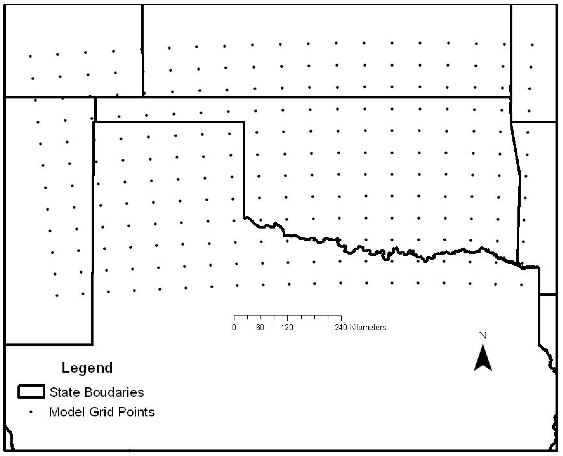
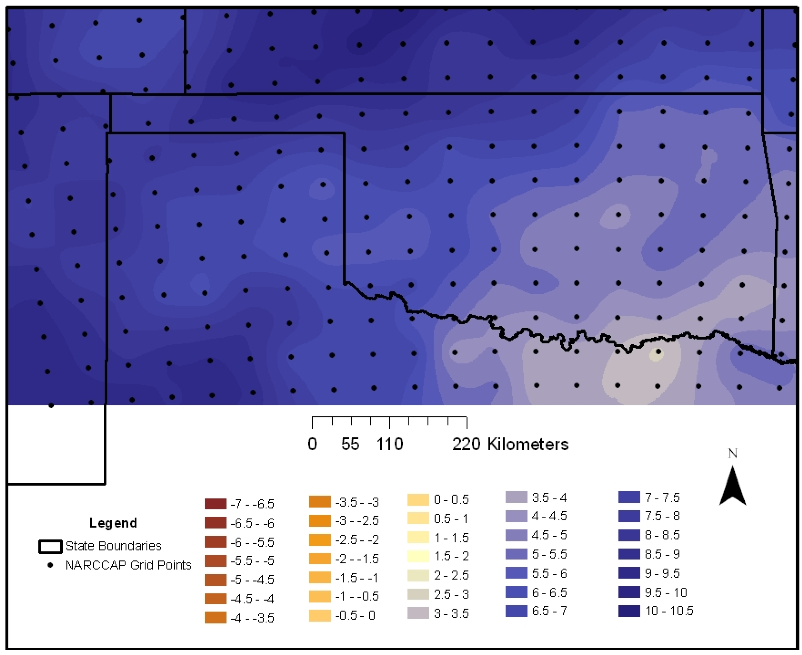
We wished to examine the impacts of potential climate change on western Oklahoma’s wind resources. We know Oklahoma has noteworthy spatial variability in its wind resource. The spatial domain of the modeled outputs used in this study was Oklahoma and small portions of surrounding states, creating a “rectangle” of latitude and longitude large enough to exhibit reasonable spatial variation
vis-à-vis the spatial scale of the modeling used (
Figure 1).
Figure 1.
Study domain showing North American Regional Climate Change Assessment Program (NARCCAP) global climate model (GCM) output grid points.
Figure 1.
Study domain showing North American Regional Climate Change Assessment Program (NARCCAP) global climate model (GCM) output grid points.
Data used in this study included:
NARCCAP GCM runs simulating past conditions from 1990 through 1999;
NARCCAP GCM output from 2039 through 2070;
A pair of wind farm locations in the domain falling in locations where projected wind velocity changes are greatest;
Oklahoma Mesonetwork wind velocity data;
Finally, the wind turbine power curve for the common 1.5-MW General Electric SLE turbine.
3. NARCCAP Output
The present study used simulated past climate data, as well as projected future wind speeds from the North American Regional Climate Change Assessment Program (NARCCAP), which implements GCMs forced with the Special Report on Emission Scenarios (SRES) A2 emission scenario. The A2 is the scenario that has been most incorporated into applied studies of future decades of the 21st century. NARCCAP is an international program devoted to regional modeling [
29], and outputs are available via open access. Although the NARCCAP models represent state-of-the-art climate modeling, some issues have been noted within the computation of temperature and precipitation patterns [
30,
31]. NARCCAP wind outputs have not been fully explored for biases, but it is likely that some may exist. Despite any limitations, the NARCCAP modeling outputs are viewed by climate scientists as robust and appeared appropriate for our purpose of examining wind farm outputs
vis-à-vis decadal changes in Oklahoma’s wind characteristics.
A portion of NARCCAP focuses on “time slice” experiments concentrating on slices of time in the past and in the future, and our study used these “time slices.” NARCCAP uses two different Global Climate Models (GCMs) for each time slice. The first represents “historical” conditions (1969–2000) modeled by the atmospheric component of the Geophysical Fluid Dynamics Laboratory’s (GFDL) GCM, known as the AM2.1 [
32].
The second time slice (2039–2070) was modeled by the Community Atmosphere Model (CAM 3.0); this is a portion of the National Center for Atmospheric Research’s (NCAR’s) GCM called The Community Climate System Model (CCSM), a coupled climate model for simulating the Earth’s climate system [
33]. Both of these sub-models contain only one component of each parent GCM: this was done so that the computational requirements of the simulations were low enough (practicable) to enable higher spatial resolution of the output.
The authors chose time slice output, because the currently available regional climate models (RCMs) were not accessible at the time we did our original work. The output from each time slice was in 50 km by 50 km grid cells. This GCM output was extracted for a subset of 228 points across our study domain. Each point represented the centroid of an output grid cell (
Figure 1).
3.1. Historical Time Slice (GFDL CM2.1)
The model that provided the simulated past output from 1969 to 2000 is the atmospheric component of the GFDL GCM. The coupled model is known as the CM2.1; however, the atmospheric component alone is known as AM2.1. These models were developed to simulate the IPCC Fourth Assessment (AR4) findings [
33]. Global coupled Atmosphere-Ocean General Circulation Models (AOGCMs) in the Coupled Model 2.x (CM2.x) family were used to expand upon the capabilities of past GFDL GCMs. One of the main goals was to create models realistically simulating phenomena from diurnal-scale fluctuations and synoptic-scale storms up to multi-century climate change [
34]. “Past” climate was based on dynamic and thermodynamic equations that represented observed conditions of the past by including natural and anthropogenic inputs not previously included ([
34], p. 304).
3.2. Climate Change Scenario
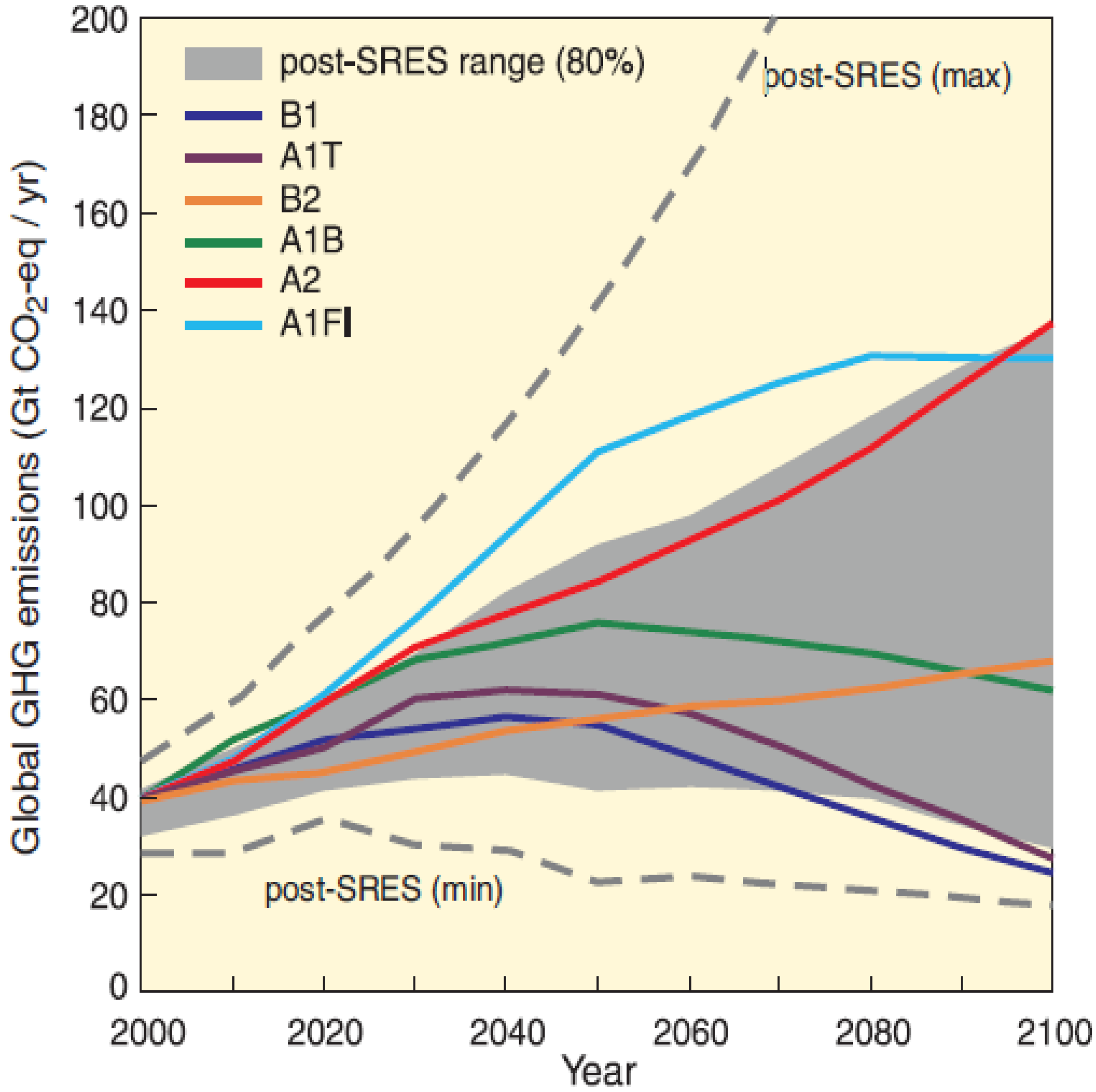
NARCCAP focused on one IPCC SRES emission scenario and, so, too, were the aims of our study. Scenario A2 was chosen from
Figure 2 due to its overall acceptance in the scientific community at the time when NARCCAP was being developed.
The A2 storyline and scenario family describes a very heterogeneous world. The underlying theme is self-reliance and preservation of local identities. Fertility patterns across regions converge very slowly, which results in continuously increasing population. Economic development is primarily regionally oriented and per capita economic growth and technological change more fragmented and slower than other storylines ([
17], p. 18).
Figure 2.
IPCC Special Report on Emission Scenarios (SRES) CO
2 emission scenarios [
17].
Figure 2.
IPCC Special Report on Emission Scenarios (SRES) CO
2 emission scenarios [
17].
3.3. Future Time Slice (NCAR CCSM3)
The Community Atmosphere Model (CAM3) is the sixth generation of atmospheric general circulation models (AGCMs) that have been developed by the climate community and NCAR. It was released to the climate community in 2004 [
35]. Like many of the GCMs that preceded it, CAM3 was designed to be a modular and versatile model that would be suitable for climate studies by the general scientific community [
35]. CAM3 can be run as a stand-alone AGCM or as the atmospheric component of the Community Climate System Model (CCSM). NARCCAP is focused on anthropogenic climate change, so the stand-alone version was implemented in the time slice experiments. This mode attempted to use accurate and detailed physics schemes “to maintain the fidelity of the simulations over a wide range of spatial resolutions and multiple dynamics” ([
35], p. 2158).
4. Wind Power Density
Changing wind speeds (one conclusion of studies of the winds of the recent past) will change wind power density. Wind power density (WPD) is the industry standard measurement of wind power potential and is measured in watts per square meter. WPD is a function of the cube of the wind speed, meaning minimal decreases in wind speed could mean significant decreases in wind energy output. WPD is defined as:
where ρ is air density and V is wind velocity [
4]. Equation (1) includes the cube of wind velocity. This means relatively small long-term increases or decreases in wind speed might have important outcomes for operating wind turbines. There is also an annual cycle of air density based on seasonal temperatures, but this is a very small effect. We used NARCCAP modeled wind and temperature outputs to make our WPD estimations.
5. Wind Farms and Mesonet Data
Wind measurements at individual wind farm turbines would have been ideal for use in this research, but wind farm owners are notoriously protective of such data, which could be used by competitors to plot the efficiency of performance. Therefore, we used proxy data from the Oklahoma Mesonetwork.
The Oklahoma Mesonetwork (Mesonet) is a network of 120 automated meteorological observation stations across all 77 counties in Oklahoma [
36]. A full suite of data is reported and quality-controlled for five-minute time increments. Wind was measured at the standard 10-m height by the RM Young wind monitor with an accuracy of ±0.3 m·s
−1 [
37].
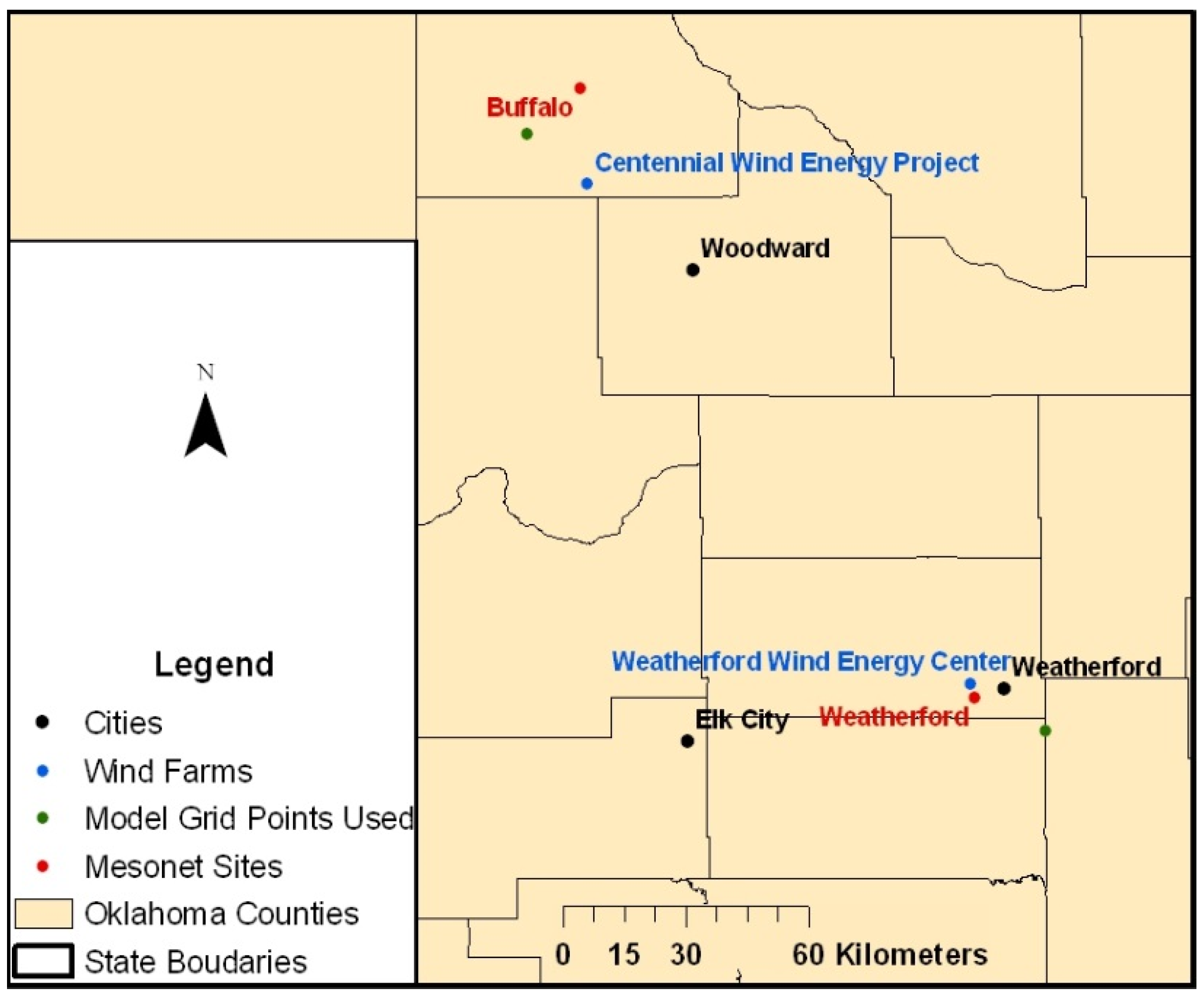
Each wind farm in Oklahoma is within 20 kilometers of a Mesonet station. We chose two wind farms in the western Oklahoma within areas of the most dramatic projected wind velocity changes in the NARCCAP output. Each wind farm was paired with the closest Mesonet station to represent that wind farm with a year of five-minute data (
Figure 3).
Figure 3.
Mesonet sites and wind farm locations.
Figure 3.
Mesonet sites and wind farm locations.
The Centennial wind farm in the northern portion of the study domain was paired with the Buffalo Mesonet station, and the Weatherford Wind Energy Center and the Weatherford Mesonet station were paired further south. See
Table 1 for wind farm information and
Table 2 for Mesonet site information.
Table 1.
Wind farms in the present study.
Table 1.
Wind farms in the present study.
| Name | Capacity (MW) | Turbines | Online |
|---|
| Weatherford Wind Energy Center (WWEC) | 147 | 98 GE SLE | May 2005 |
| Centennial Wind Farm | 120 | 80 GE SLE | December 2006 |
Table 2.
Oklahoma Mesonet station characteristics.
Table 2.
Oklahoma Mesonet station characteristics.
| Name | County | Latitude (°) | Longitude (°) | Elevation (m) |
|---|
| Buffalo | Harper | 36.83 | −99.64 | +559 |
| Weatherford | Custer | 35.50 | −98.77 | +538 |
6. Power Calculations
Characteristics of the 1.5-MW General Electric (GE) SLE wind turbine [
38], one of the most widely-used turbine in the United States, were used to calculate the harvest of wind from the modeled winds. Power curves and cut-in and cut-out speeds for the GE 1.5 MW turbine were applied.
The Mesonet wind data were vertically extrapolated to the GE turbine height of 80 m using the standard wind power law equation:
where U was the estimated wind velocity at 80 m. U
R was the wind velocity at the Mesonet tower height of 10 m multiplied by the ratio of height desired above the ground (Z = 80 m) over the reference height (Z
R = 10 m). The ratio was raised to the alpha (α = 0.143) ([
39], p. 390). This ratio, then, was an approximation of vertical speed shear under average conditions.
Once the wind velocities were extrapolated to turbine height, we made power generation calculations.
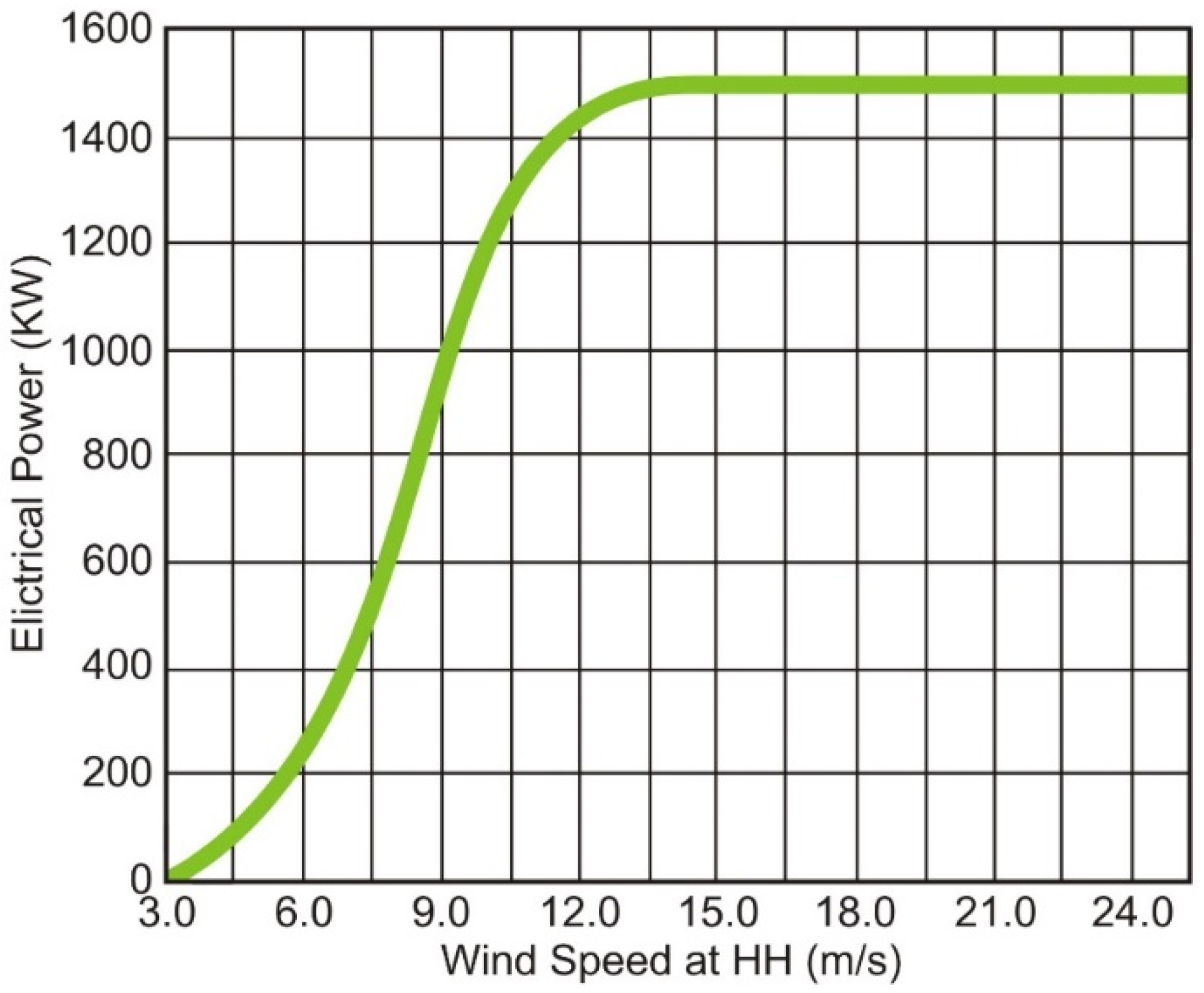
Figure 4 shows the relationship between wind velocity and power generated for the GE 1.5 MW SLE turbine type. HH is the hub height of the turbine.
Figure 4.
Power curve for GE 1.5sle 1.5 MW turbine [
27].
Figure 4.
Power curve for GE 1.5sle 1.5 MW turbine [
27].
We utilized a cubic polynomial equation that represented this wind turbine’s power curve:
where C
1, C
2, C
3 and C
4 are the coefficients or the power curve for this turbine type and V
1 is the reference wind-speed value for each coefficient [
40]. Wind speeds of greater than 25 m·s
−1 were excluded, as this is the automatic cut-out speed for the GE 1.5 MW SLE turbine. Far less than 1% of all observations were over 25 m·s
−1. We experimented with various ways to achieve a best fit, including consideration of non-parametric transformations, but we found that Equation 3 provided the best fit to the observations.
7. Outputs for the Study Domain
Model output was extracted from NARCCAP’s database [
18]. The study domain (
Figure 1) had 228 grid cells of 50 km by 50 km. Cell centroids were assigned values of the NARCCAP output and mapped. The NARCCAP output for each centroid was three-hour averages of 10-m instantaneous wind velocity simulations. For each yearly centroid file, there were 2920 wind values, one observation for every three-hour output. Seasons were defined via the standard atmospheric practice [
41]. December through February was winter; spring was March through May; summer was June through August; and fall was September through November.
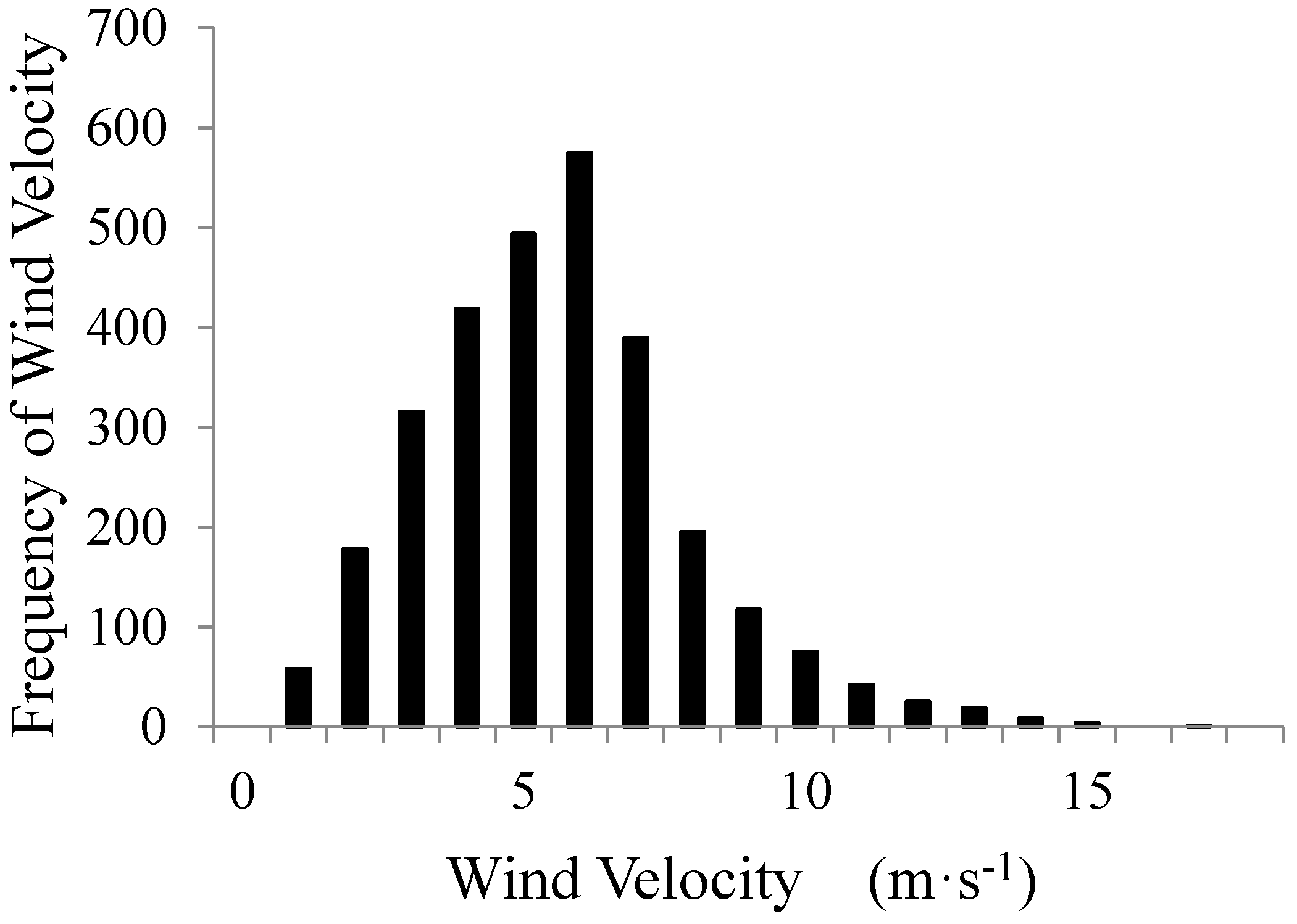
Figure 5 exhibits the wind velocity distribution for 1990 through 1999 at one of the NARCCAP grid cell centroids. In all bar graphs in this article, wind data have been arranged into discrete “bins”, as specified in the figure captions. The skewness of such wind distributions is well known [
42].
Figure 5 is not a normal distribution; it is skewed and characteristic of all of the centroids in the study domain. Therefore, we used the medians of all distributions as measures of central tendency, as is the usual practice in the wind literature and wind industry.
Figure 5.
1999 NARCCAP 10-m wind velocity simulations at the Buffalo wind farm grid point. Wind speed categories are labeled with their upper bounds. “1” represents 0–1 m·s−1; “2” is up to 2 m·s−1, etc.
Figure 5.
1999 NARCCAP 10-m wind velocity simulations at the Buffalo wind farm grid point. Wind speed categories are labeled with their upper bounds. “1” represents 0–1 m·s−1; “2” is up to 2 m·s−1, etc.
Median velocities were averaged by year and season for each decade, and percent changes in wind velocity medians were calculated for three future decades by comparing them to the 1990–1999 decade. The percent change formula was:
where “New median” refers to modeled output for a future decade and the “Old median” is from the 1990–1999 data.
8. GIS and Spatial Statistics
The NARCCAP outputs were processed and input into a geographic information system (GIS) for statistical analyses and visual representation. The averaged decadal median wind velocities were mapped by season and by whole decade, resulting in five maps for each of the four decades examined. Only selected maps are shown in this article.
We used kriging as a method to facilitate the ease of interpretation of our maps. In recent decades, kriging has become a fundamental tool in geostatistics. There are three main theoretical assumptions within kriging: (1) first-order stationarity, in which the mean is constant over space with the study domain; (2) second-order stationarity, where covariance depends only on distance and direction apart, not locations; and (3) the distribution of the data are normally distributed ([
43], p. 119). Assumptions (1) and (2) were satisfied via using standard geospatial techniques. Normality (3) was assessed via
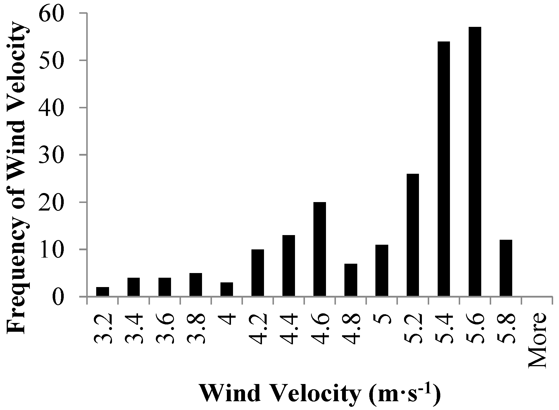
Figure 6.
Figure 6 displays the averaged median wind velocity value for all 228 grid points in the study domain for 1999; the distribution is not normal. We applied several data transformations, but none improved the distribution in a useful way nor markedly changed our power calculations. Our experience shows non-normality to be common in wind data from Oklahoma and elsewhere, and geospatial analysis has been used in many other wind applications. Although we recognize this may introduce some bias into the analysis, kriging is nevertheless appropriate for the visual map interpolation of the grid point data.
Figure 6.
1999 NARCCAP simulated 3-h averaged wind velocities at 10 m over all 228 grid points.
Figure 6.
1999 NARCCAP simulated 3-h averaged wind velocities at 10 m over all 228 grid points.
Ordinary kriging with a spherical semivariogram model was used for all of our map outputs. Spherical models are most often used unless there is some overriding concern, and in this case, there did not appear to be. We used this kriging approach to horizontally interpolate the data at each grid point in order to produce all of the maps of this study.
The percent change in averaged median wind velocity was calculated for each season per decade for each grid cell in the domain. The two wind farms (
Figure 3) were in the region with the greatest changes by decade. These two wind farm locations have similar landscape conditions with open, rural land with low population densities and similar elevations. The locations varied in elevation by 21 m and are approximately 142 km apart.
Both wind farms use GE 1.5 MW SLE commercial wind turbines, so they are directly comparable in power calculations. Due to the restraints associated with real data and the practices of other wind power studies, five-minute Mesonet observations were used.
The NARCCAP grid points closest to each Mesonet site (
Figure 3) were chosen to represent the change in wind velocity per season, per decade for future decades. The distance between the Buffalo Mesonet site and Centennial wind farm is 23 km, and the distance between the Weatherford Mesonet site and the Weatherford Wind Energy Center (WWEC) is 4 km. The distance between the Centennial wind farm and the closest NARCCAP grid point is 16.9 km, and the distance between the WWEC wind farm site and the closest NARCCAP grid point is 19.3 km.
9. Findings
We believe NARCCAP median wind velocity patterns for 1999 in the region of the two wind farms were realistic in representing Oklahoma’s observed wind climate, as known from other research [
27]. The modeled winds presented the strongest wind velocities in western Oklahoma and decreased southward and eastward through Oklahoma. This is partially an effect of surface geography, where there is considerably more forest and hills, providing increased surface friction in the eastern part of the study domain.
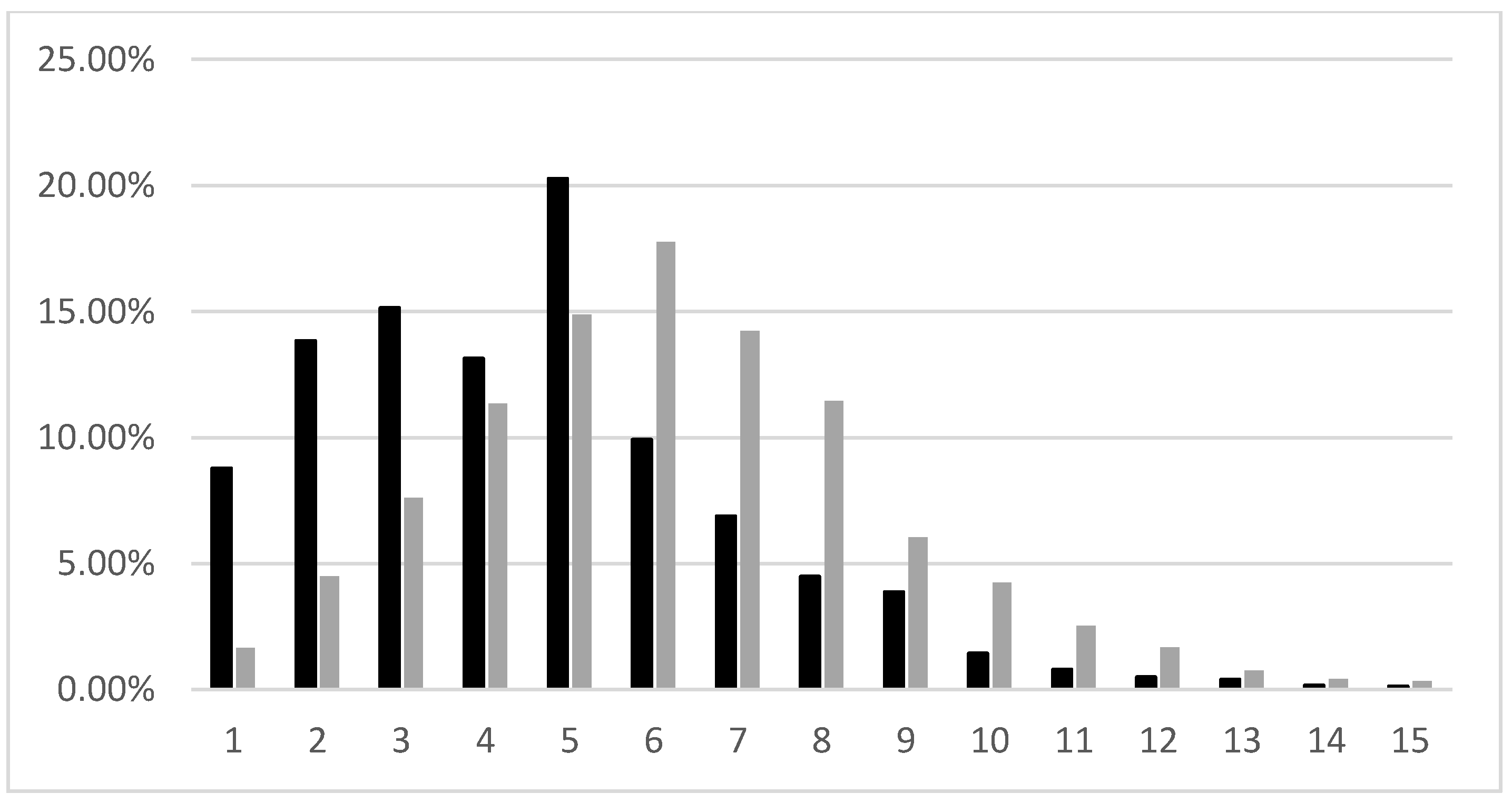
Figure 7 is the relative frequency distribution of the 1999 10-m modeled grid point wind velocities and the corresponding Buffalo Mesonet site’s wind velocities. Note that these data represent, respectively, five-minute Mesonet data and three-hour NARCCAP output, so the Mesonet observations are actually 36-times as plentiful. The distributions are largely similar. The 1999 Mesonet annual median wind velocity was 3.6 m·s
−1, and the corresponding NARCCAP grid point had an annual median wind velocity of 5.5 m·s
−1. The Mesonet measured some “calm” conditions at the lower end of the 0–1 m·s
−1 bar graph bin, as anemometers do not term at very low wind speeds; NARCAPP had a minimum of 0.14 m·s
−1. Thus, NARCCAP estimates higher wind velocities, in part due to the nature of the difference between the time and spatial domains of the two datasets.
There are three mitigating factors making us believe that NARCCAP estimates are sufficient for our purposes. First, the Mesonet site and the grid point are approximately 20 kilometers apart, and there are some small differences in landscape shape and altitude. Second, the shapes of the distributions are quite similar; the skewness of both distributions is 0.98. Third, the greatest departures between the distributions are in the low wind speeds. As power ramps up with wind speed (see the turbine characteristics in
Figure 4), the lowest categories of wind speed shown in
Figure 9 have small impacts on the total decadal power production we calculated in
Section 11.
Figure 7.
1999 relative frequencies of the Buffalo Mesonet site (black) and the nearest NARCCAP grid point (gray). Wind speed categories are labeled with their upper bounds. “1” represents 0–1 m·s−1; “2” is up to 2 m·s−1, etc.
Figure 7.
1999 relative frequencies of the Buffalo Mesonet site (black) and the nearest NARCCAP grid point (gray). Wind speed categories are labeled with their upper bounds. “1” represents 0–1 m·s−1; “2” is up to 2 m·s−1, etc.
Thus, comparison of Mesonet 1999 observational data and NARCCAP modeled outputs seems to indicate that the NARCCAP model is sufficient for our limited purpose. The 1999 seasonal maps (not reproduced here) of Mesonet versus NARCCAP modeled median wind velocity patterns are also similar to each other.
9.1. 2040–2049 Changes in Wind Velocity
The annual percent change in median wind velocities between 1999 and 2040–2049 was greatest in western Oklahoma. However, the seasons varied in terms of changes in generation. For 2040–2049, spring and summer are the seasons that show the biggest modeled percent change wind velocity at the wind farms.
Table 3 shows the percentage change in wind velocity by season for this decade at each wind farm.
Table 3.
Percentage changes in wind velocities at each wind farm for each modeled decade compared to 1990–1999.
Table 3.
Percentage changes in wind velocities at each wind farm for each modeled decade compared to 1990–1999.
| Period | Centennial Wind Farm | WWEC |
|---|
| | 2040–2049 | |
| Winter | 0.44 | 0.39 |
| Spring | 8.38 | 6.19 |
| Summer | 6.37 | 5.25 |
| Fall | 1.21 | −1.05 |
| | 2050–2059 | |
| Winter | 0.19 | 0.44 |
| Spring | 6.36 | 6.13 |
| Summer | 4.22 | 4.74 |
| Fall | −2.43 | −2.21 |
| | 2060–2069 | |
| Winter | 0.25 | 0.68 |
| Spring | 7.32 | 7.70 |
| Summer | 6.58 | 5.91 |
| Fall | −1.37 | −1.73 |
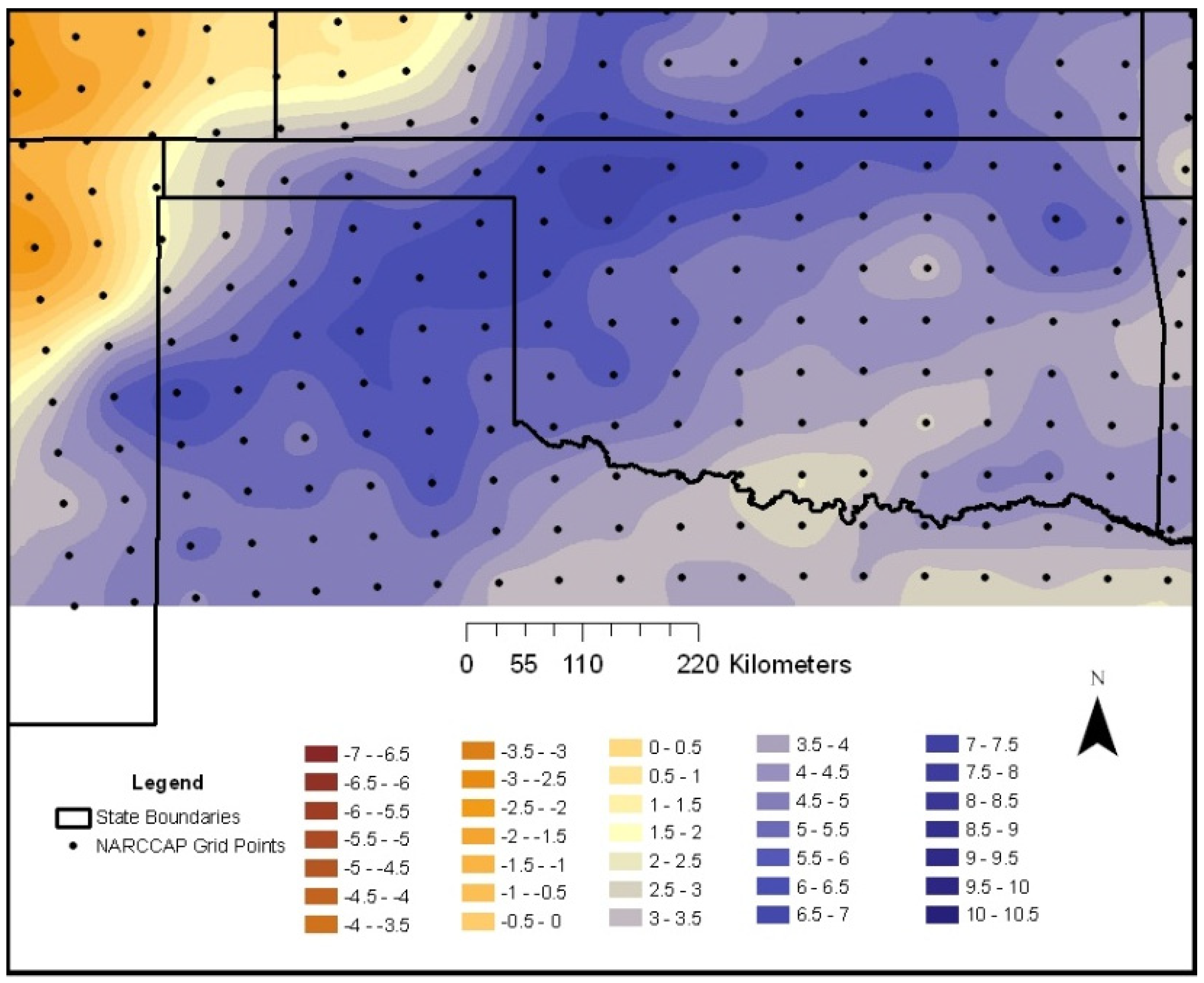
In spring 2040–2049 (
Figure 8), there is an increase in wind velocity from southeast to northwest over the entire study domain. This pattern affects both wind farms, especially the Centennial wind farm in northwestern Oklahoma. In the 2040–2049 summer, the maximum increase in wind velocity is along a southwest to northeast diagonal in the western portion of the study domain (
Figure 9).
An important note is that in all outputs from all future decades we examined, the order of absolute relative strengths of winds were spring, winter, fall and summer. This was unchanged from the 1990–1999 base decade.
Figure 8.
Percentage change in simulated spring 2040–2049 wind velocity at 10 m.
Figure 8.
Percentage change in simulated spring 2040–2049 wind velocity at 10 m.
Figure 9.
Percentage change in simulated summer 2040–2049 wind velocity at 10 m.
Figure 9.
Percentage change in simulated summer 2040–2049 wind velocity at 10 m.
9.2. 2050–2059 Changes in Wind Velocity
For this decade, the overall median wind velocities show the least change from 1999 over most of the study domain and are changed less than the 2040–2049 decade. However, the seasonal variations are again noticeable (
Table 3). Specifically, spring and fall display the biggest changes in magnitude of wind velocities for this decade with the largest increases in the spring and decreases in the fall.
During spring (
Figure 10), the highest positive increase in wind velocities occurs in western Oklahoma. Areas where there are smaller increases in positive percent change include northeastern Oklahoma. These patterns could again be a result of baroclinicity (thermal gradients) being displaced further south. Thus, an increase in strong, windy spring cold fronts moving southeastward through the study domain could be responsible for the southwest to northwest band of strongest change running through the western part of the state.
Figure 10.
Percentage change in simulated spring 2050–2059 wind velocity at 10 m.
Figure 10.
Percentage change in simulated spring 2050–2059 wind velocity at 10 m.
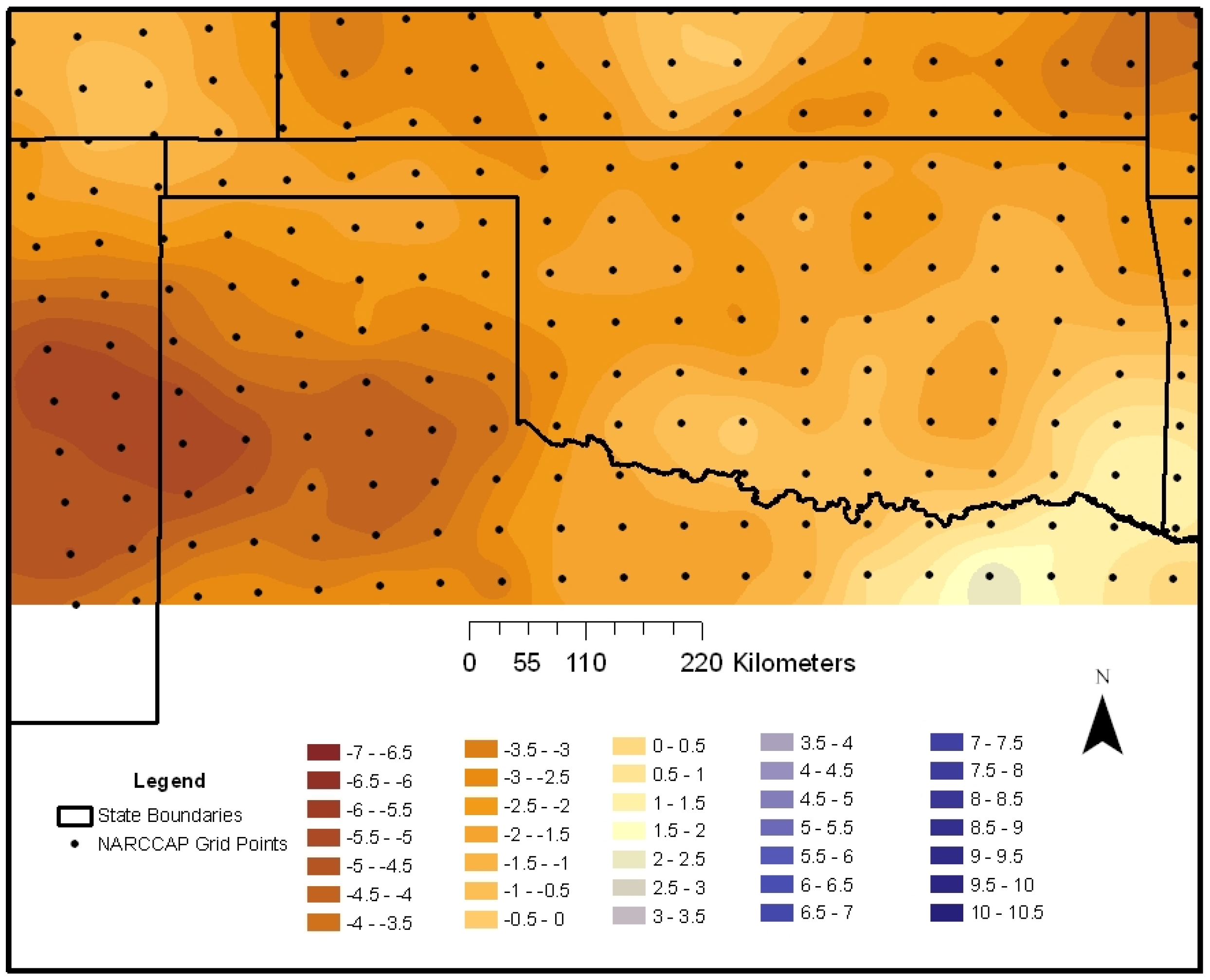
Fall 2050–2059 (
Figure 11) is the counterpoint of spring in that the patterns show a negative change in wind velocities over the study domain. The greatest magnitude of change occurs in the far western portion of the study area. Again, this could be a result of summer upper-level storm tracks shifting further north, therefore not making it into the study domain as often as in the present. Results from fall 2050–2059 match speculation that areas of the southern United States could see a decline in wind velocities [
5]. However, this decrease is not extended to the annual period as a whole.
Figure 11.
Percentage change in simulated fall 2050–2059 wind velocity at 10 m.
Figure 11.
Percentage change in simulated fall 2050–2059 wind velocity at 10 m.
9.3. 2060–2069 Changes in Wind Velocity
The final future decade examined shows percent change patterns that are the farthest in time and are the largest when compared to 1999. Some wind velocities in
Table 3 show changes of over 7%.
There are, again, important seasonal differences to be considered.
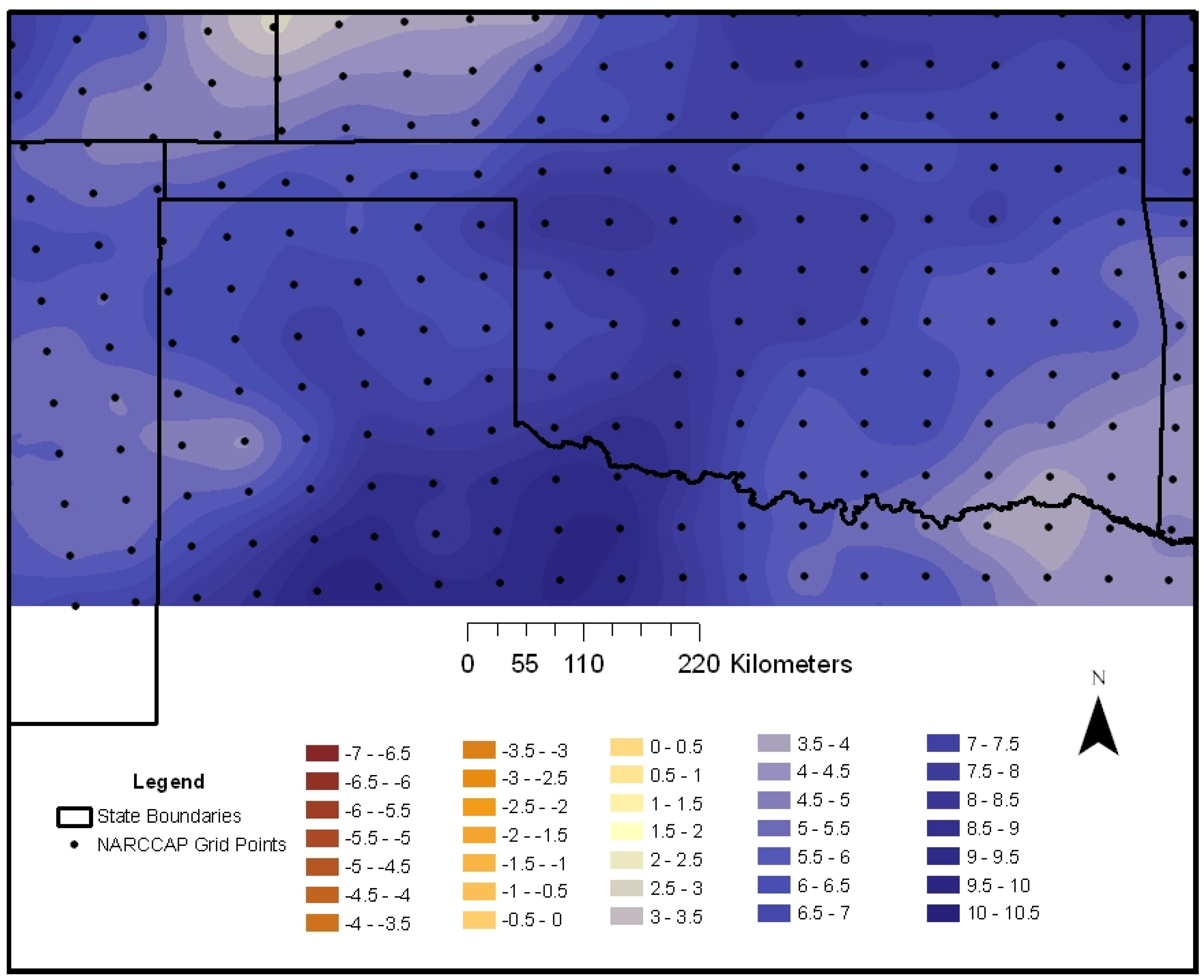
Table 3 shows positive seasonal percentage changes in all seasons, but fall, with spring and summer having the largest positive changes. In spring 2060–2069 (
Figure 12), the highest magnitude percent increases in median wind velocity are across the central and southwestern portions of Oklahoma, including both wind farm locations chosen for study.
Figure 12.
Percentage change in simulated spring 2060–2069 wind velocity at 10 m.
Figure 12.
Percentage change in simulated spring 2060–2069 wind velocity at 10 m.
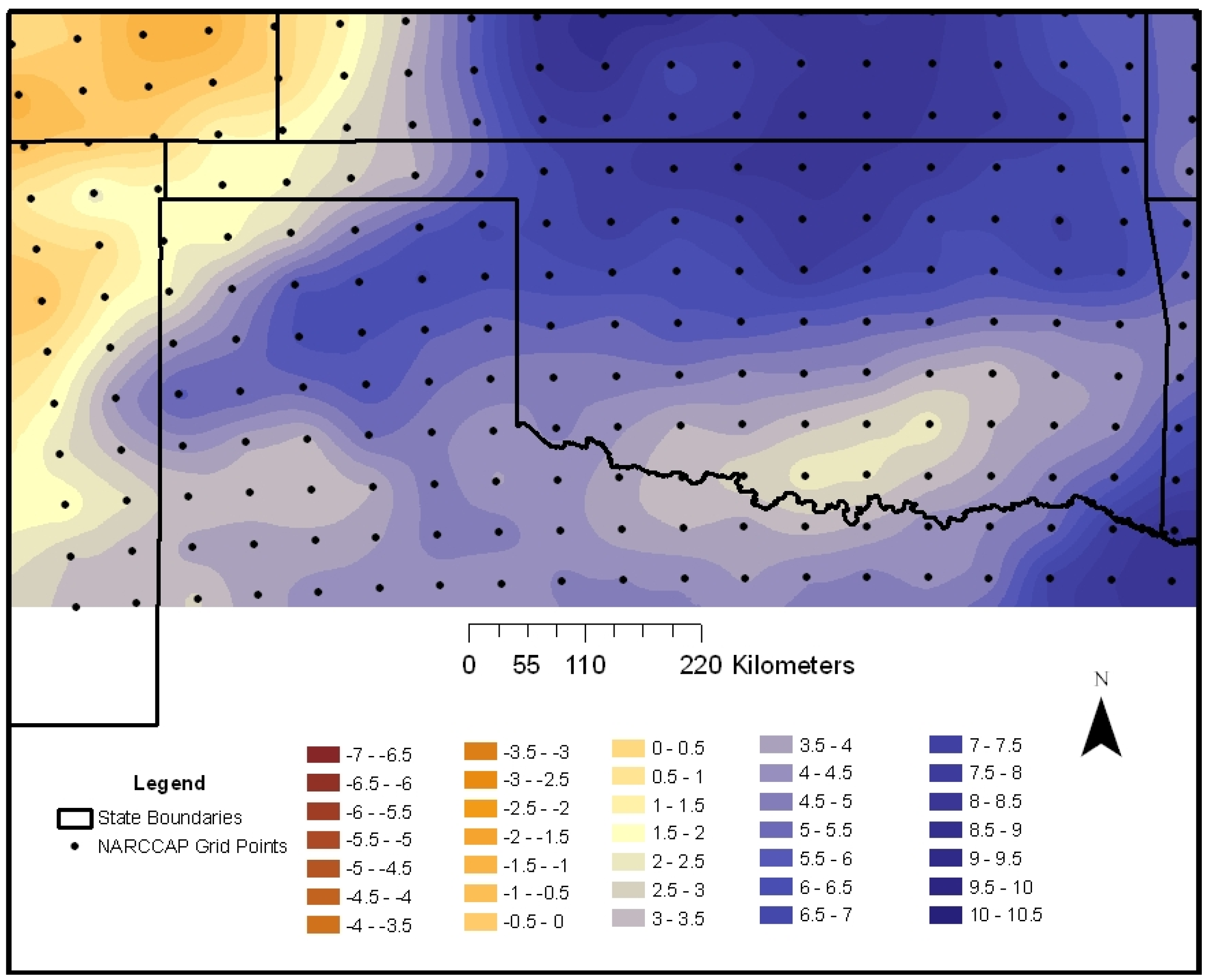
The spatial pattern in the 2060–2069 summers (
Figure 13) is similar to the 2040–2049 and 2050–2069 decadal patterns, except enhanced and displaced southward. Possibly, climatological patterns of dominating high-pressure systems shifting southward could explain this pattern, where baroclinicity would move further south along the clockwise surface circulation associated with high-pressure systems. As in the other decades, the actual wind velocities are weakest in the summer.
Interestingly, summer shows steep gradients of change to the northwest and southeast of the two example wind farm sites. For summer, there is a definite regional advantage located in the western portion of the main body of Oklahoma.
Figure 13.
Percentage change in simulated summer 2060–2069 wind velocity at 10 m.
Figure 13.
Percentage change in simulated summer 2060–2069 wind velocity at 10 m.
10. Reasons for Wind Velocity Increases
Our work was not focused on deconstructing NARCCAP modeling to discern the exact mechanisms that increase future wind speeds of western Oklahoma in most seasons. However, we made a cursory examination of the NARCCAP temperature and wind patterns over our study domain and found increased baroclinicity associated with the future seasons of increased wind speeds. Baroclinicity refers to horizontal gradients in temperature over short horizontal distances, both at the surface and aloft [
44]. In our study domain, these temperature gradients are directly related to the spatial patterns of the strongest flow in the first few kilometers of the atmosphere.
11. Power Generation
We calculated power generation for the base decade of 1990–1999 and the three future decades of 2040–2049, 2050–2059 and 2060–2069 for each of the two wind farms. After this was completed, the percent changes in power output per decade were compared to the base decade.
The NACCAP model output provided 1999 as its single reanalysis year, and accordingly, we used 5-min wind observations for 1999 to represent the entire decade of 1990–1999. This also made sense in the context of Oklahoma’s Mesonetwork, which started its observations in 1994. There was no indication of 1999 being unrepresentative of the 1990–1999 decade.
To compare our total decadal power calculations between the 1990–1999 base decade and future decades, we multiplied the sum of the 1999 wind observations by 10 to represent the 1990–1999 decadal averages. Both the Mesonet observations and NARCCAP outputs were divided into annual and seasonal periods.
Equation (2) was used to extrapolate the 10-m Mesonet observations to the GE wind turbine height of 80 m. Winds have a bit different nature at 80-m hub height than at 10-m because of the diurnal rise and fall of the frictional turbulence of the boundary layer. However, other western Oklahoma data from a tall tower not at either of the subject wind farms showed that over a year, the Pearson r2 between the two time series exceeded 98%. Since the Mesonet wind data were only taken at 10-m and we wanted an “apples-to-apples” comparison of Mesonet data with NARCCAP output, we choose to extrapolate both of these data types to 80 meters to make comparisons.
The extrapolated winds were used to calculate the power generated from the GE 1.5-MW wind turbine power curve. The power law wind profile Equation (2) used included the exponent alpha (α = 0.143), which represents near-neutral atmospheric stability and relatively flat, smooth Earth surface to characterize the near-surface layer of the atmosphere [
5]. Vertical wind speed shear changes for other stability conditions were not used, because they were imponderable based on extrapolated Mesonet 10-m observations and very sparse tall tower data from western Oklahoma.
Using the 5-min Mesonet data, we calculated the 1999 annual and seasonal power generation per turbine in kilowatt hours (kWh). The resulting values were multiplied by the number of turbines in each wind farm and then multiplied by ten years to estimate total gross power generated for an entire wind farm for the base decade of 1990–1999. Save for multiplication by 10, the same procedure was done to calculate the total potential power generation for each of the future decades 2040–2049, 2050–2059 and 2060–2069. The final step calculated the percent change from 1990 to 1999 to each future decade using Equation (4), except substituting the percent change in potential power for median wind velocities.
The estimates included cut-in and cut-off speeds of this particular turbine type. However, they did not account for operational practices of the operators (maintenance, etc.) and curtailments by grid operators. These factors are unknowable into the future and could be different between the two wind farms. For simplicity, we compared only the gross possible power in order to highlight wind changes due to climate change.
11.1. Power Generation Changes
Our potential power calculations are shown in megawatt hours (MWh) for each decade as a whole and then by season for the 1990–1999 base decade (
Table 4). Examination of seasonal values is instructive because of the definite differences between seasons.
In
Table 5, the Centennial wind farm shows increases in power generation for every season in every decade, except in the fall seasons of 2050–2059 and 2060–2069. Each future decade has higher potential power generation than 1990–1999. The largest percent increase in power generation is in the summer for 2040–2049, in the spring for 2050–2059 and in the summer for 2060–2069.
Table 4.
1990–1999 gross potential power generation from the Centennial wind farm.
Table 4.
1990–1999 gross potential power generation from the Centennial wind farm.
| Period | Potential Gross Production (MWh) * |
|---|
| Decadal | 1,871,930 |
| Winter | 446,084 |
| Spring | 612,360 |
| Summer | 424,913 |
| Fall | 388,574 |
Table 5.
Gross potential power from the Centennial wind farm for future decades.
Table 5.
Gross potential power from the Centennial wind farm for future decades.
| Period | Power Output (MWh) * | Change from 1990 to 1999 (%) |
|---|
| 2040–2049 |
| Decadal | 2,091,756 | 11.74 |
| Winter | 452,490 | 1.44 |
| Spring | 728,151 | 18.91 |
| Summer | 508,848 | 19.75 |
| Fall | 402,268 | 3.52 |
| 2050–2059 |
| Decadal | 1,994,232 | 6.53 |
| Winter | 447,574 | 0.33 |
| Spring | 701,335 | 14.53 |
| Summer | 481,112 | 13.23 |
| Fall | 364,211 | −6.27 |
| 2060–2069 |
| Decadal | 2,046,492 | 9.33 |
| Winter | 447,859 | 0.40 |
| Spring | 712,054 | 16.28 |
| Summer | 510,814 | 20.22 |
| Fall | 375,766 | −3.30 |
Table 6 and
Table 7 show a positive percent change, similar seasonal characteristics and higher generation values for the WWEC. However, WWEC has less total percent change than the Centennial wind farm. The WWEC wind farm has more turbines than the Centennial wind farm, so the potential gross production is larger. It appears that the seasonal wind velocity changes force the WWEC wind velocities into more efficient portions of the power curve (
Figure 4), therefore generating more wind power with similar percent change patterns. At both wind farms, fall wind generation is projected to slacken as compared to the base decade.
Our major conclusion is that these two Oklahoma wind farms have significant overall potential wind power generation benefits to reap from a globally warming climate. This might provide a bit of an interstate economic advantage if western Oklahoma sees overall increases while much of the rest of the United States experiences lower velocities.
As time goes on and world carbon emissions continue to increase, as assumed in the NARCCAP model, most seasons will see power increases. Yet, the differences might be unequal by season, and this, in itself, poses interesting questions for the management of power loads given electrical heating and cooling demands of the various seasons.
Table 6.
1990–1999 gross potential power generation from the WWEC.
Table 6.
1990–1999 gross potential power generation from the WWEC.
| Period | Potential Gross Production (MWh) * |
|---|
| Decadal | 5,044,161 |
| Winter | 1,212,052 |
| Spring | 1,390,705 |
| Summer | 1,237,841 |
| Fall | 1,203,563 |
Table 7.
Gross potential power from WWEC for future decades.
Table 7.
Gross potential power from WWEC for future decades.
| Period | Power Output (MWh) * | Change from 1990 to 1999 (%) |
|---|
| 2040–2049 |
| Decadal | 5,325,627 | 5.58 |
| Winter | 1,224,257 | 1.01 |
| Spring | 1,537,220 | 10.54 |
| Summer | 1,384,929 | 11.88 |
| Fall | 1,179,220 | −2.02 |
| 2050–2059 |
| Decadal | 5,275,866 | 4.59 |
| Winter | 1,22,4819 | 1.05 |
| Spring | 1,536,485 | 10.48 |
| Summer | 1,365,021 | 10.27 |
| Fall | 1,149,541 | −4.49 |
| 2060–2069 |
| Decadal | 5,364,803 | 6.36 |
| Winter | 1,227,644 | 1.29 |
| Spring | 1,561,284 | 12.27 |
| Summer | 1,406,503 | 13.63 |
| Fall | 1,169,371 | −2.84 |
11.2. Capacity Factor
The decade gross power as given above does not tell the entire story.
Table 6,
Table 7 and
Table 8 are exaggerations of the wind power that could actually be reaped from the wind. Sometimes, wind is very weak, and turbines do not turn at all, while at other times, the wind is not blowing enough to generate at the turbine’s nameplate-rated capacity. At various other short periods of time, the Oklahoma wind blows faster than the design limits of this turbine type, and the blades are “feathered” to prevent damage.
To quantify wind farm generation compared to the theoretical maximum electricity that could be generated, there is a value known as the capacity factor. The capacity factor is a ratio between actual power generated by a turbine compared to its output if it was running at 100% capacity all of the time. Typical wind power capacity factors are 20% to 40% ([
45], p. 1). In western Oklahoma, some locations exceed 40%, making them very attractive in terms of the relatively short time needed to recoup investment.
In our study, the capacity factors for the GE 1.5 MW SLE commercial wind turbine show small increases for future decades (
Table 8). Capacity factors relate to payback times for turbine investment. These results tell us that the changes in winds as modeled do not have a deleterious effect on these wind farms. It is evident that the nature of the winds at the WWEC wind farm place the WWEC in the “sweet spots” of the GE 1.5-MW SLE power generation curve more often than at the Centennial wind farm (
Figure 4).
Table 8.
Capacity factors for the wind farms as calculated from NARCCAP output.
Table 8.
Capacity factors for the wind farms as calculated from NARCCAP output.
| Period | 1990–1999 | 2040–2049 | 2050–2059 | 2060–2069 |
|---|
| | | CENTENNIAL WIND FARM | | |
| Spring | 0.23 | 0.28 | 0.27 | 0.27 |
| Summer | 0.16 | 0.19 | 0.18 | 0.19 |
| Fall | 0.15 | 0.15 | 0.14 | 0.14 |
| Winter | 0.17 | 0.17 | 0.17 | 0.17 |
| Total | 0.18 | 0.20 | 0.19 | 0.19 |
| | | WWEC WIND FARM | | |
| Spring | 0.53 | 0.58 | 0.58 | 0.59 |
| Summer | 0.47 | 0.53 | 0.52 | 0.54 |
| Fall | 0.46 | 0.45 | 0.44 | 0.44 |
| Winter | .46 | 0.47 | 0.47 | 0.47 |
| Total | .48 | 0.51 | 0.50 | 0.51 |
12. Potential Climate Change Impacts on Oklahoma’s Wind Industry
These results hint at potential positive impacts on Oklahoma’s wind power industry and economy. This does not mean we expect better wind generation conditions in all of Oklahoma, nor at all times. The point is that modeled outcomes strongly suggest spatial heterogeneity in wind climate changes in our study domain. This is a cautionary tale for wind farm development now moving eastward through the state.
It is well known that Oklahoma has some of the best potential for wind power generation in the world and the modeled promise of improvement. Our results do not necessarily mean a strong gravitation to invest in Oklahoma wind farms as opposed to other states or regions not so blessed. Federal and state regulatory and tax structures will ultimately mediate in any geographic shift of investment.
The results of this study indicate that there could be significant changes in wind power generation resulting from climate change in western Oklahoma. For all future decades studied, there was an increase in total power generated from the wind. The findings are of some note, because we suggest that the wind resource might increase in areas where there are favorable winds already and because this is the first Oklahoma study to suggest increases in wind power generation. We have presented a caveat to the accepted overview that climate change will be detrimental to wind resource development in the United States at large. As models improve, we expect a richer geographic exploration of regional projections and their meaning for wind power.


