1. Introduction
Airborne Light Detection and Ranging (LiDAR) is an active remote sensing technique used to acquire 3D representations of objects with very high resolution [
1,
2]. LiDAR systems emit short laser pulses to illuminate the Earth’s surface and then capture the reflected light with photodiode detectors. By measuring the laser flight time propagating through the medium, a distance to target (range) can be determined assuming a known constant speed of light in the medium [
3,
4]. With superior performance for acquiring 3D measurements and easy deployment, LiDAR data has been used for many scientific applications such as biomass estimation, archaeological application, power line detection, and earth science applications including temporal change detection [
5,
6,
7,
8].
A conventional discrete-LiDAR system records only a few (
5) discrete-returns for each outgoing laser pulse. A hardware ranging method called constant fractional discrimination (CFD) [
9] is implemented in most current LiDAR systems to discriminate vertically cluttered illumination targets along the laser path [
10]. With critical requirements for vertical resolution and the advancement of processing and storage capacity over last decade, Full Waveform LiDAR (FWL) has emerged as a viable alternative to discrete-LiDAR. FWL records the entire digitized backscatter laser pulse received by detector with very high sampling rate (1–2 GHz) [
11].
FWL was introduced in commercial topographic LiDAR systems in 2004 and a number of LiDAR systems now have the capability to store the entire digitized return waveform [
12,
13,
14]. FWL enables better vertical resolution because discrete-return LiDAR resolution is largely influenced by laser pulse width or Full Width at Half Maximum (FWHM) [
10,
15]. However, sophisticated digital signal processing methods are required to extract points and other target information (e.g., radiometry) from current FWL systems. To date, many full waveform processing algorithms have been proposed and are widely used in the research community. An overview of waveform processing techniques can be found in [
11]. Gaussian decomposition [
16,
17,
18] and deconvolution [
15,
19] are two processing strategies that have been applied in a number of previous studies. Hartzell
et al. [
20] proposed an empirical system response model which is estimated from single return waveforms over the dynamic range of the instrument. The empirical response is then used as a template for actual return waveforms, resulting in improved ranging.
Recently, the analysis of FWL processing has focused on evaluating the different methods in parallel to find superior algorithms for specific applications. For example, Wu
et al. [
21] compared three deconvolution methods: Richardson-Lucy, Wiener filter, and nonnegative least squares to determine the best performance using simulated full waveforms from radiative transfer modeling; the Richardson-Lucy method was found to have superior performance for deconvolution of the simulated full waveforms. Parrish
et al. [
10] presented an empirical technique to compare three different methods for full waveform processing: Gaussian decomposition, Expectation-Maximization (EM) deconvolution and a hybrid method (deconvolve-decompose). Using precisely located screen-targets in a laboratory, they arrived at the conclusion that no single best full waveform method can be found for all applications.
Despite the recent focus on applications of FWL for topographic studies, it was first evaluated for the processing of LiDAR bathymetry [
22]. Recently, however, full waveform bathymetric LiDAR has not received much attention in the literature, especially compared to topographic FWL. This is likely due to the lack of available bathymetric LiDAR datasets for the scientific community and the more complicated modeling required for LiDAR bathymetry to compensate for factors such as water surface reflection and refraction, water volume scattering and turbidity that can complicate the propagation models and attenuate return strength resulting in a lower signal to noise ratio (SNR). Water volume scattering can be difficult to rigorously model, especially for shallow water environments where water surface backscatter, water volume scattering, and benthic layer backscattering are mixed into a single complex waveform that makes discrimination of individual responses from a single return difficult [
23]. The complex waveform signals in a bathymetric environment demand a noise-resistant and adaptive signal processing methodology. In order to reduce the complexity of bathymetric LiDAR, multiple wavelengths (usually a NIR LiDAR system for water surface detection, and a green LiDAR system for water penetration) systems are normally used to facilitate benthic layer retrieval [
12]. For example, Allouis
et al. [
24] compared two new processing methods for depth extraction by using near-infrared (NIR), green and Raman LiDAR signals. By combining NIR and green waveforms, significantly more points are extracted by full waveform processing and better accuracy is achieved. Even though multi-wavelength LiDAR systems are common for bathymetry, single band systems have emerged recently as well [
14,
25,
26]. Wang
et al. [
27] has compared several full waveform processing algorithms for single band shallow water bathymetry using both simulated and actual full waveform data, and concluded that Richardson-Lucy deconvolution performed the best of the tested waveform processing techniques. However, the performance with the actual full waveform data was not verified with comparison to external high accuracy truth data. There have also been several studies which have examined the performance of single band full waveform bathymetry using simulated LiDAR datasets. Abady
et al. [
23] proposed a mixture of Gaussian and quadrilateral functions for bathymetric LiDAR waveform decomposition using nonlinear recursive least squares. Both satellite and airborne configurations were simulated and examined and showed significant improvement for bathymetry retrieval, however, the simulation has not to date been validated with observations from real-world studies, especially for very shallow water bathymetry in turbid conditions. The performance of full waveform LiDAR in shallow water has received little attention in the literature beyond the study by McKean
et al. [
25]. Limited water depths and significant turbidity impose challenges for bathymetric LiDAR, especially for longer pulse width laser systems where water surface, water column and benthic layer returns mix together. A bathymetric full waveform processing strategy to account for the longer pulse width and the excessive noise present in the bathymetric waveform would enable more accurate bathymetry determination.
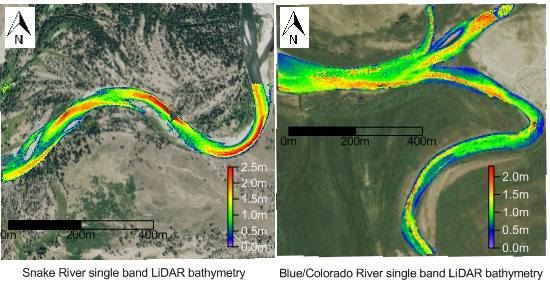
In this paper, we first propose a novel full waveform processing algorithm using a continuous wavelet transformation (CWT) to decompose single band bathymetric waveforms. The seed peak locations acquired from CWT are then used as input to both an empirical system response (ESR) algorithm and a Gaussian decomposition method. As a benchmark for comparison, a common Gaussian decomposition algorithm is also used with candidate seed locations acquired from second derivative peaks, similar to that presented in [
17,
18]. The waveform processing methods are applied to two distinct fluvial environments with varying degrees of water turbidity. Water depths extracted from both a discrete point cloud and full waveform processed point clouds are then compared to water depths measured in the field with an Acoustic Doppler Current Profiler (ADCP). Finally, we analyze the accuracy of water surfaces extracted from discrete point clouds and full waveform processed point clouds using both green wavelength and near-infrared detected water surfaces compared to GNSS RTK field measurements. The rest of the paper is organized as follows:
Section 2 presents the waveform processing mathematical models and the procedure used for water depth generation from the LiDAR observations,
Section 3 provides a description of the airborne datasets and ground truthing used to evaluate the processing methodology, and
Section 4 presents the experimental results. The paper closes with a discussion of the study conclusions and areas for future research.
2. Method and Mathematical Model
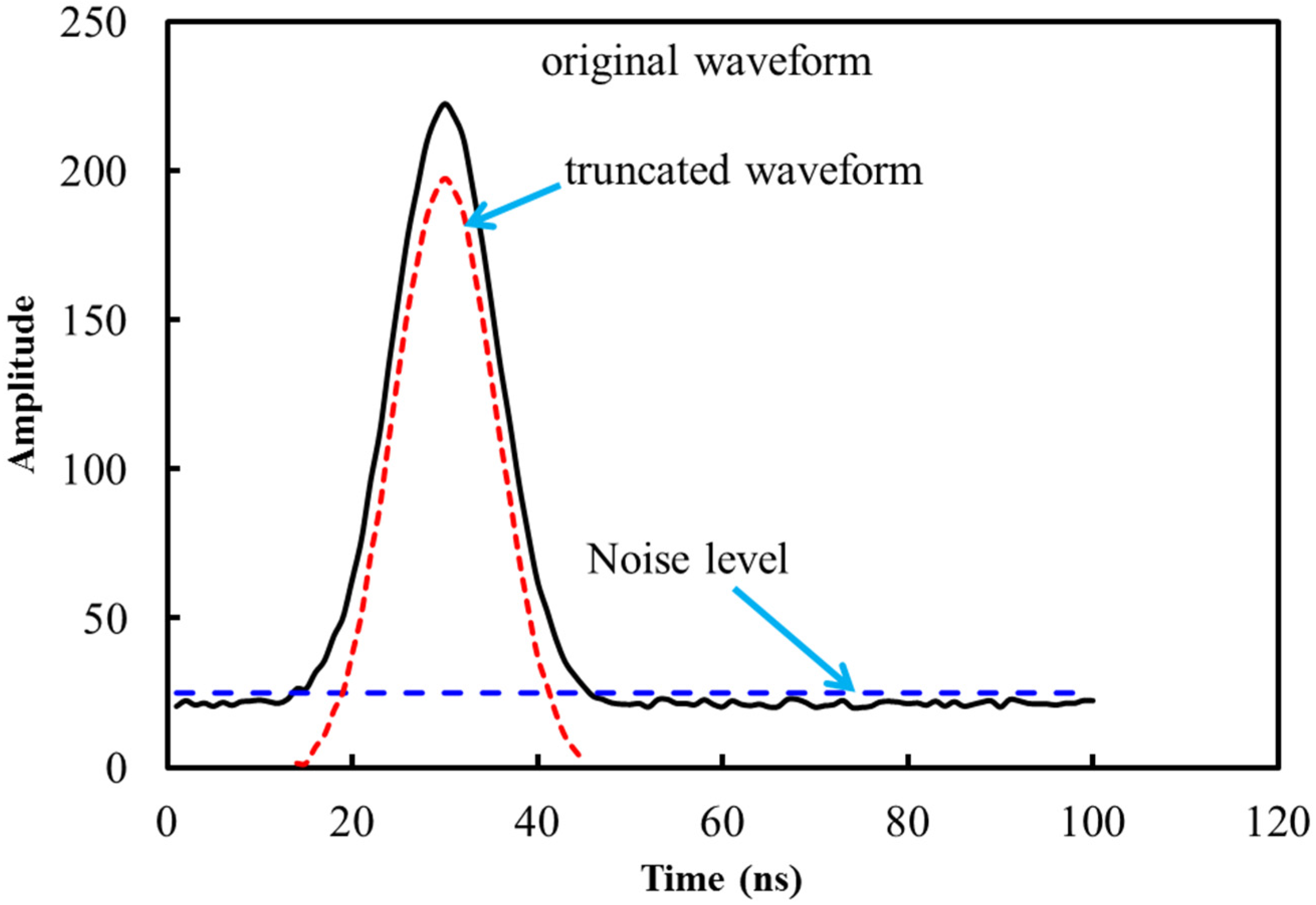
FWL return profiles are normally a fixed length discrete time signal containing backscatter information for a large region of interest. For return profiles where the echoes are clustered in a short range window, a significant portion of the full waveform does not carry useful information (
i.e.
, the profile represents the noise threshold); an effective method to pre-process the full waveforms that removes this extraneous information from the original waveform will reduce the total amount of processing time required. A noise level can be defined as the minimum amplitude and can be estimated from the full waveform data itself; for example as the median absolute deviation for each waveform [
28]. For our study, amplitudes within 10% of the return gate are considered as the noise level (
Figure 1). The return gate is an instrument specific configuration parameter used to reduce the effect of sun glint and noise returns. Herein, all the bins below the noise level were removed, and only the remaining signal was examined. The removal of data below the noise threshold significantly speeds up the calculations due to the decreased data volume to be analyzed. It should be noted that bathymetric LiDAR waveforms can have quite complicated return energy profiles. To demonstrate this, representative samples of bathymetric waveform are given in
Figure 2.
Figure 1.
Pre-processing of the return waveform by removing data below the noise threshold of the original waveform. The noise level is defined as 10% above the return gate which is given by the manufacturer specifications. The truncated waveform is saved for posterior processing.
Figure 1.
Pre-processing of the return waveform by removing data below the noise threshold of the original waveform. The noise level is defined as 10% above the return gate which is given by the manufacturer specifications. The truncated waveform is saved for posterior processing.
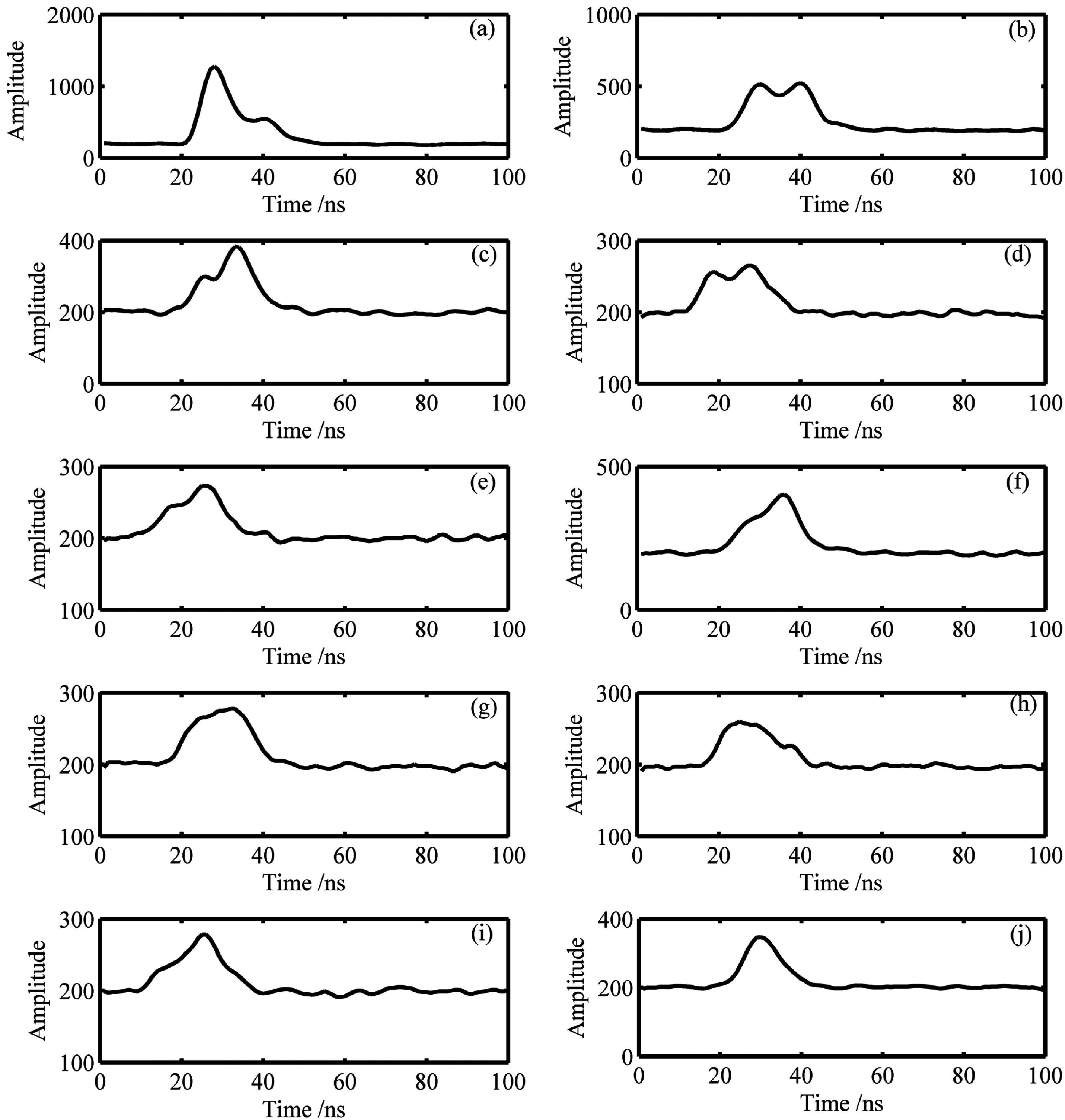
Figure 2.
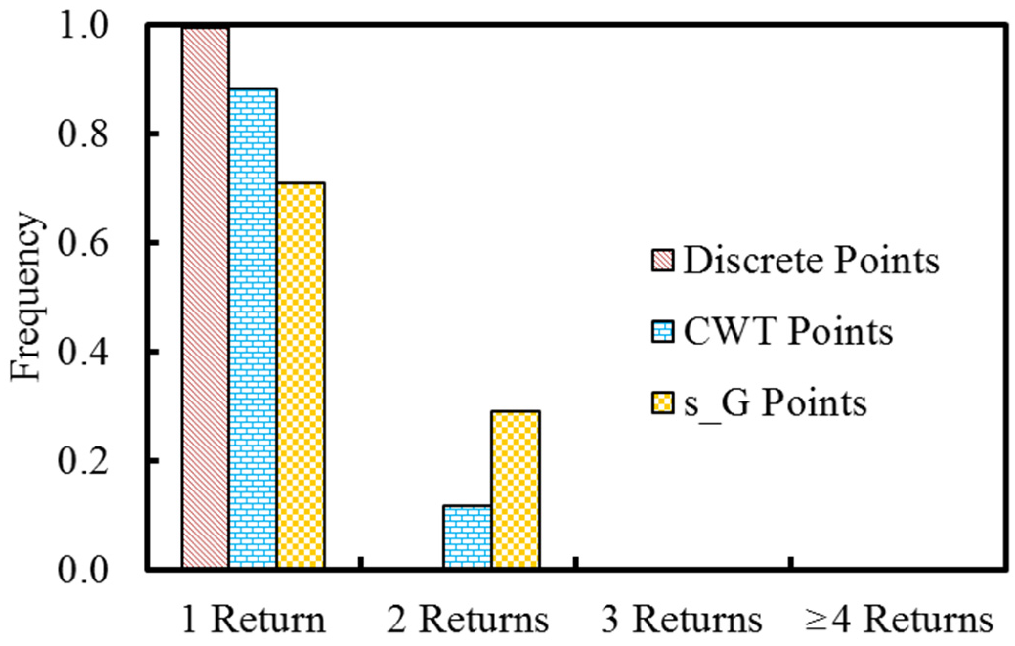
Typical bathymetric return waveforms. (a–d) are from clear water with multiple visible peaks of varying peak amplitude; (e–f) contain more subtle evidence of multiple peaks; (g–i) contain multiple peaks that overlap and are visibly not discernible; (j) contains a single peak. Multiple peaks are critical for benthic layer retrieval as the first return is normally the water surface and the latter return more probably from the benthic layer.
Figure 2.
Typical bathymetric return waveforms. (a–d) are from clear water with multiple visible peaks of varying peak amplitude; (e–f) contain more subtle evidence of multiple peaks; (g–i) contain multiple peaks that overlap and are visibly not discernible; (j) contains a single peak. Multiple peaks are critical for benthic layer retrieval as the first return is normally the water surface and the latter return more probably from the benthic layer.
2.2. Gaussian Decomposition Method
Gaussian decomposition is a popular approach for FWL processing as it can simultaneously provide estimation of peak locations and widths. Gaussian decomposition is implemented using Expectation-Maximization (EM) in this study. EM is an iterative method, normally used in signal and image processing, to estimate the maximum probability for a set of parameters of a statistical model. As the name indicates, there should be an expectation (E) step and a maximization (M) step, and EM iterates between the E step and the M step until a convergence criterion is satisfied [
28,
32].
A LiDAR waveform return can be represented as the sum of multiple Gaussian distributions [
17], and mathematically this can be expressed as:
Here,
is the full waveform that is the sum of the Gaussian components with multiple components (
) and
is time,
represents a Gaussian component with an individual mean (
) and a standard deviation (
). The number of peaks and the initial peak locations are needed as initial values for the EM algorithm described by the following equations:
Here,
is the relative weight of the component distribution
;
is the probability that sample belongs to component ;
is the amplitude for sample ;
is the number of samples in the waveform;
is the mean peak location; and
is the standard deviation for that component, proportional to the pulse width or FWHM.
As EM is a local maximum searching method, peaks with spurious
µi or
σi are removed to ensure a reasonable result. Also, extremely weak returns, for example, peaks with
pi less than 0.05 are removed to guarantee algorithm convergence. From Equations (2)–(5), it is evident that EM is actually a Gaussian decomposition because its underlying model is a Gaussian mixture model. For the purpose of assessing performance of Gaussian decomposition with different seeding peak locations, both CWT detected peak locations and peaks acquired from second derivative analysis [
18] are applied to initialize EM estimation.
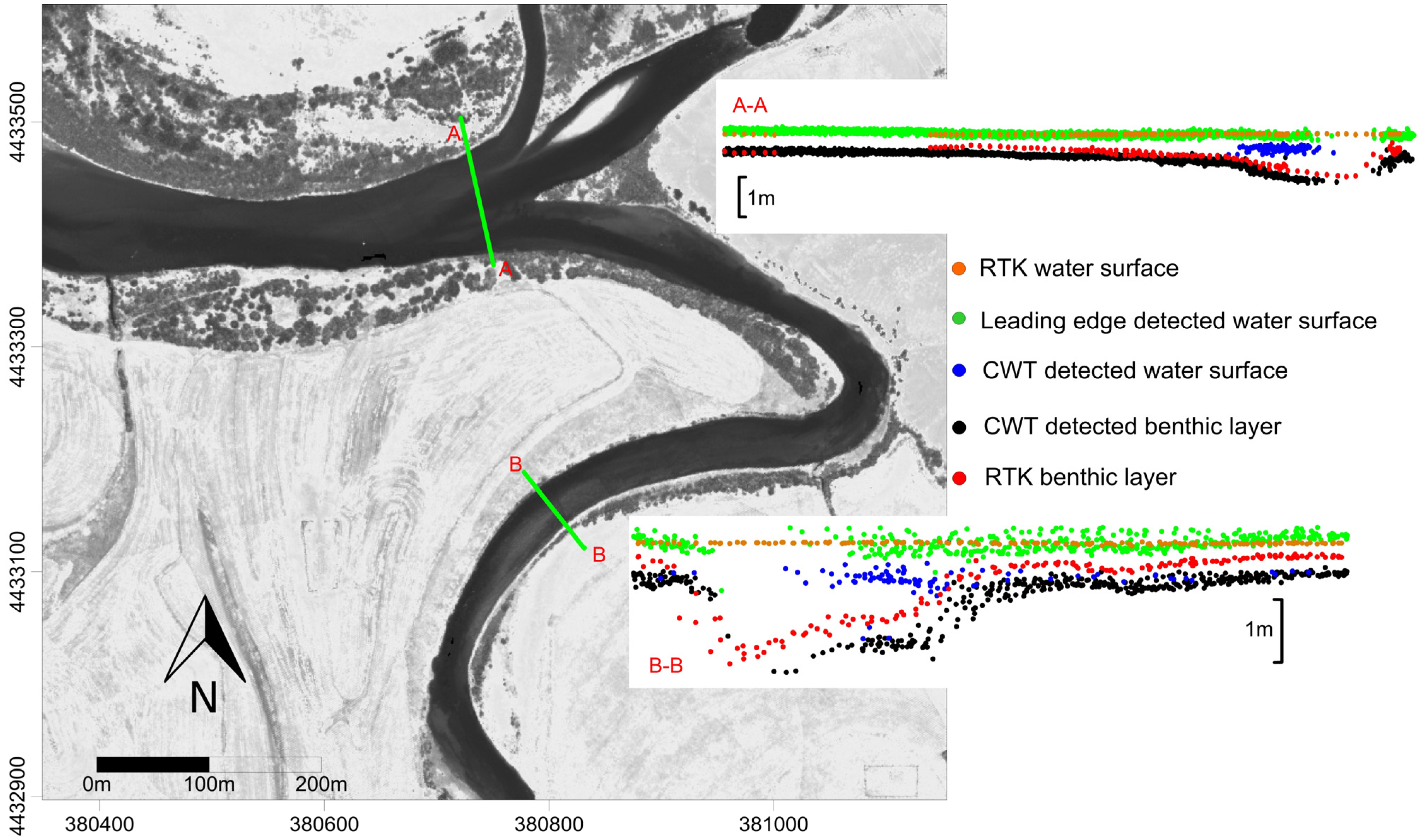
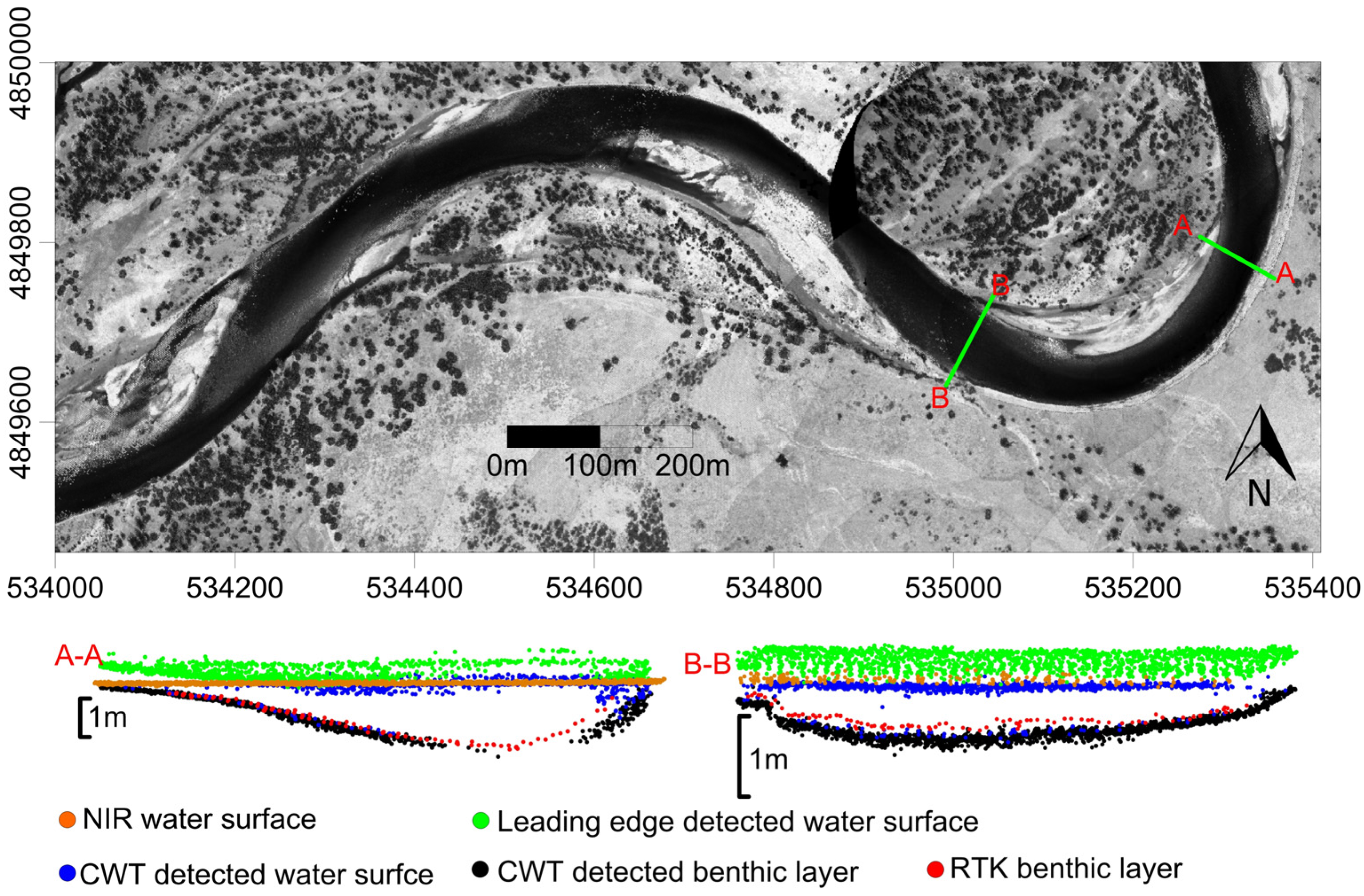
2.4. Water Depth Generation
As the field measurements used in the paper are water depths records collected with an Acoustic Doppler Current Profiler (ADCP), we need to infer water depths from the 3D LiDAR points as a basis of comparison. We also need to segment the raw point clouds from each of the target extraction techniques to separate water column and bottom returns and properly identify the benthic layer. The basic strategy for benthic classification is to first classify the last of multiple returns as initial candidate benthic returns, and then use a region growing method with the initial benthic points and regionally lowest elevation points to refine the total benthic surface points using the TerraScan software package. The classification algorithm is similar to that used to determine ground returns in topographic LiDAR surveys and is based on the methodology presented in [
34]. It should be noted that each of the green LiDAR returns from below the surface of the water has been corrected for both refraction of the pulse at the air/water interface, and for the change in the speed of light within water [
22]. To define the water boundary, a fluvial river-line is acquired from aerial orthoimages by visually identifying and digitizing the land/water border.
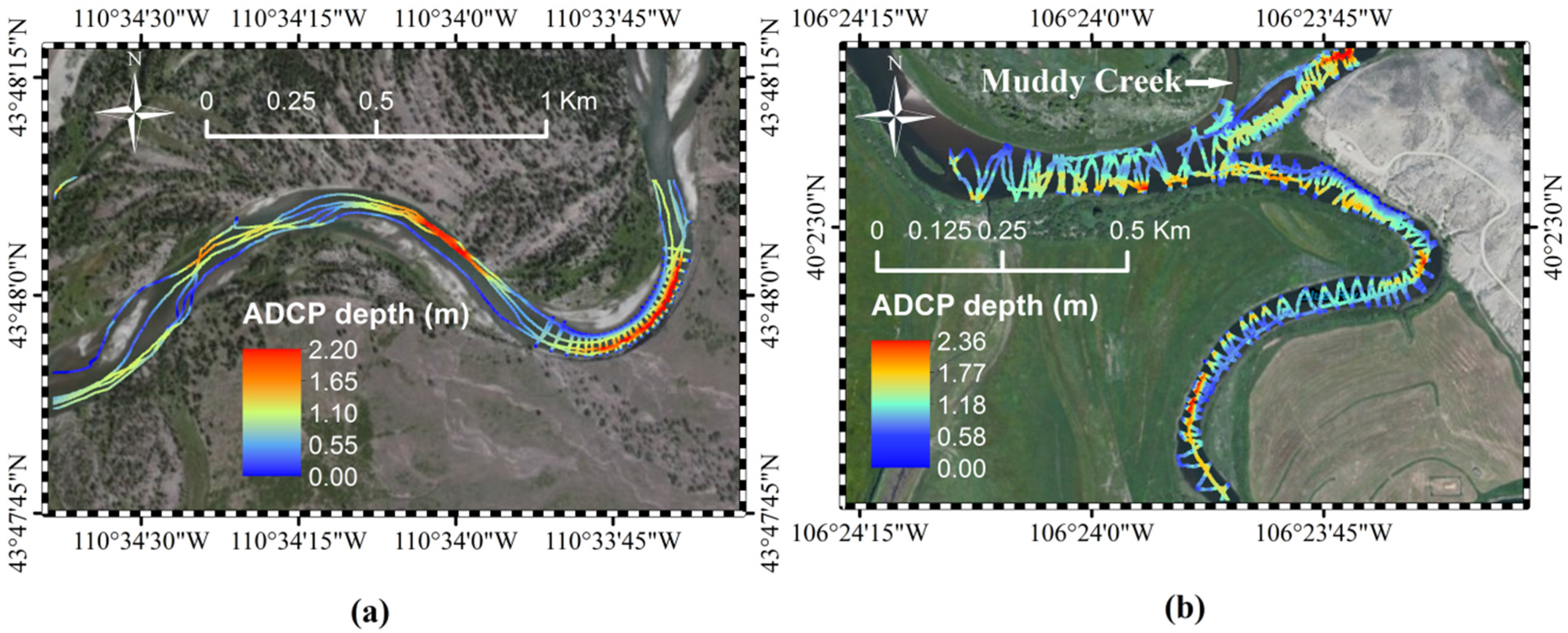
To convert the benthic layer points extracted from the point cloud to water depths, a water surface is required to subtract the benthic layer elevation from the water surface elevation for each benthic point. To highlight the differences in depth determination between single and multiple bands bathymetric LiDAR sensors we examine two realizations of the water surface for each river: The first water surface is extracted from alternative sources (NIR water surface for the Snake River, RTK water surface for the Blue/Colorado River) and the second water surface is extracted from each of the green LiDAR point clouds alone. For green LiDAR point clouds, the water surface can be defined as the remaining LiDAR returns within the boundary of the water body after benthic classification. The NIR water surface was acquired by extracting all NIR returns within the water boundary, as NIR LIDAR can theoretically only be retro-reflected from the water surface [
35].
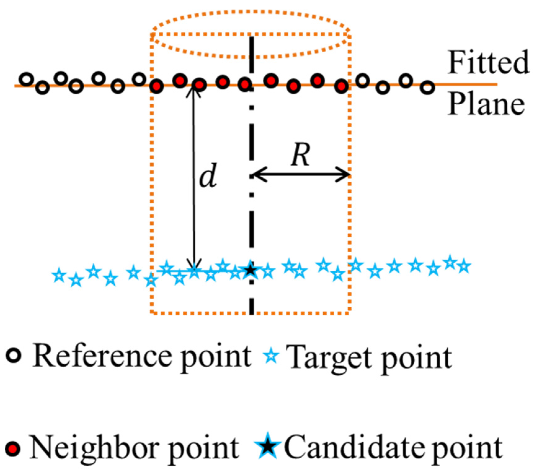
Figure 4.
Definition of point to plane distance. For each target point, the neighbor points are those within the cylinder with a radius of . A fitted plane is constructed by least squares estimation, and the distance of the candidate point to the fitted plane is defined as the point to plane distance.
Point clouds created by airborne LiDAR are generally irregularly distributed, and therefore conventional image processing techniques which assume raster input are not suitable for posterior analysis. As an alternative, we utilized a point to plane distance to compute the distances between an individual LiDAR returns and its neighbor points [
36].
Figure 4 shows the schematic steps to compute the point to plane distance. For each specific candidate point, neighbor points are selected within the cylinder with specific searching radius
, and thus a fitted plane is constructed by least squares estimation. The distance from the candidate point to the fitted plane is defined as the point to plane distance
. The point to plane distance is used in this study to calculate the water depth given a cloud of water surface (reference points) and benthic points (target points).
5. Discussion
Full waveform LiDAR processing is able to produce a significantly denser point cloud with more multiple return reflections than CFD for bathymetry. The ability to recover multiple returns by the waveform methods is especially significant, because the additional returns are more probable benthic returns for fluvial environments. The multiple returns can also benefit the classification of benthic layer as the last return of multiple returns are assigned as the seed benthic positions for the region growing classification algorithms. This algorithm is different from the method proposed by Allouis
et al. [
24] who used NIR returns to estimate the water surface; here the mixed LiDAR signal produced by water surface and water bottom reflections was directly processed through the CWT to extract both surface and benthic locations. One of the challenges for single band bathymetric LiDAR is to recover both the water surface and bottom position from the full waveform. The longer pulse width laser used in the Aquarius system exacerbated the mixture of water surface, water column and benthic returns. In the future we plan to examine our methodology on short pulse width bathymetric full waveform LiDAR systems such as the Riegl VQ 820-G, AHAB Hawkeye III, EAARL, and Optech Titan.
The results of the study also suggest that there is no superior full waveform processing algorithm for all bathymetric situations which agrees with the conclusions of Parrish
et al. [
10]. ESR performed the best in the Snake River using a NIR water surface, with an R
2 of 0.92 and the lowest Std. of 13 cm. However, the c_G and CWT results for the Snake River with the NIR surface were statistically quite similar to the ESR results. With a green water surface the CWT performed marginally better than ESR with R
2 of 0.92
vs. 0.88, both with a Std. of 14 cm vs. 14 cm. LiDAR for the Blue/Colorado River did not perform nearly as well as the Snake River study due to the significant water turbidity. CWT water depths with either an RTK or green water surface gave the best performance (R
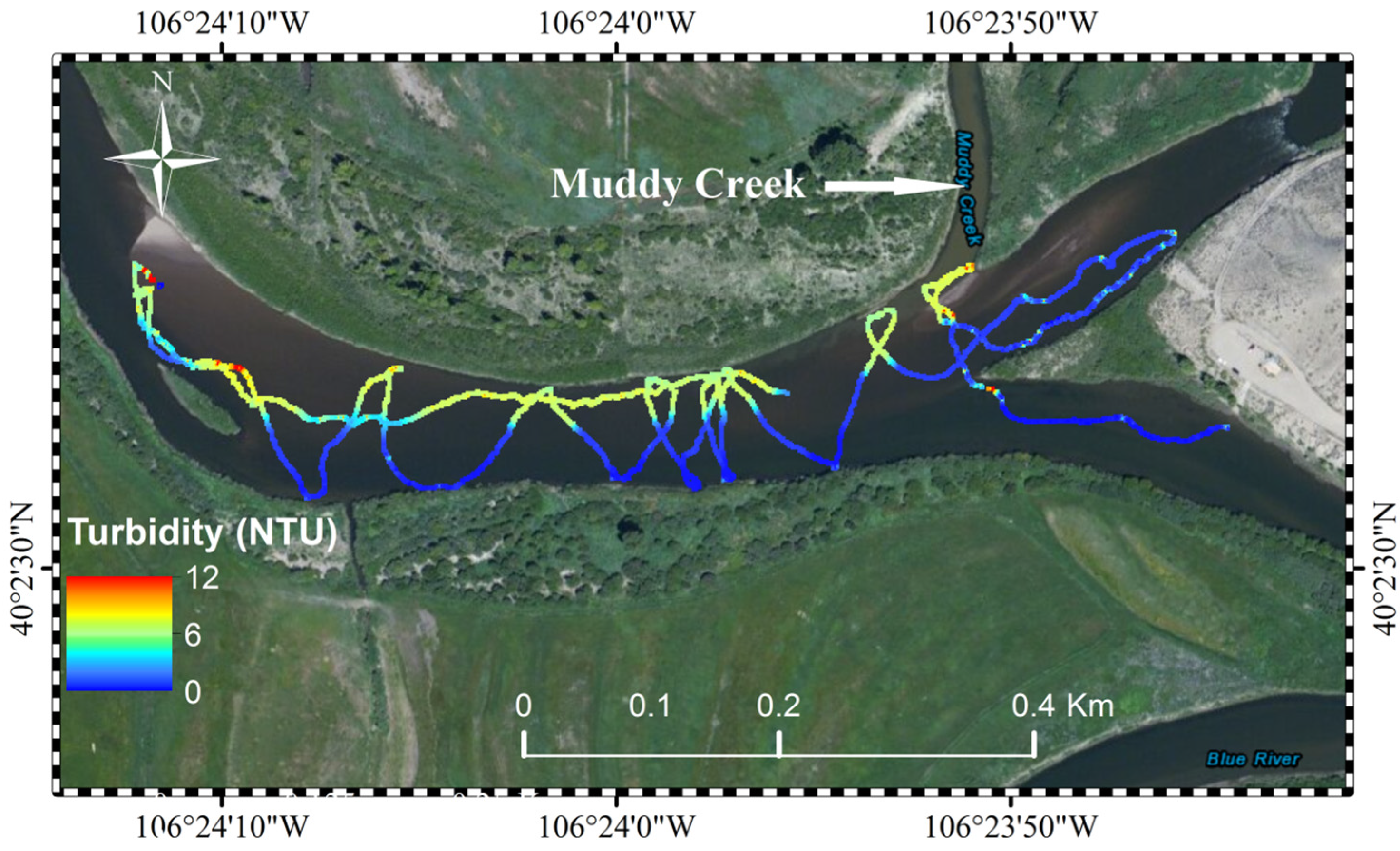
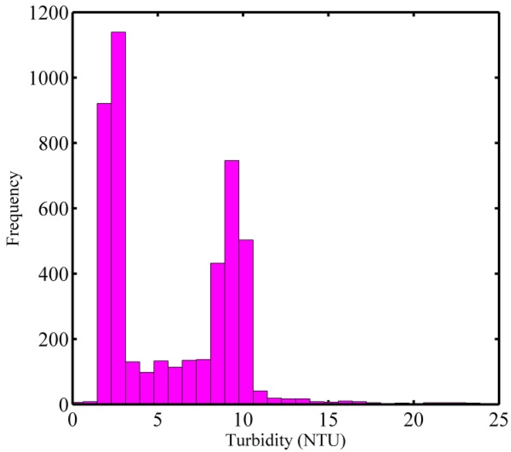
2 of 0.57 and 0.58, respectively). In general the approaches that model expected signal shape (Gaussian and ESR) performed quite poorly for the Blue/Colorado River, suggesting that the water turbidity causes significant distortion to the return waveform shape. Based on this we can safely conclude that CWT is more stable than the other full waveform processing algorithms for shallow water fluvial environments. Both the ESR and CWT showed good bathymetric performance for difference cases, confirming that it is critical for commercial software to include a variety of full waveform processing strategies. However, unfortunately, the optimal processing strategy is not available
a priori, and therefore a certain level of performance assessment is necessary for users to determine the best processing strategy for their study conditions.
We have also compared water surfaces estimated by both NIR and Green LiDAR returns. There is a definite vertical bias between the two surface estimates. The comparison of the NIR and green water surfaces for the Snake River study showed a maximum mean vertical offset of 45 cm and 33 cm of Std. for ESR. The minimum average of 18 cm of vertical offset and 10 cm Std. are observed for the discrete green water surface. Overall, it appears that the NIR water surface gives slightly better results than using a green surface (for clear water). Turbid water greatly degraded the green water surface performance with large mean error (s_G: 82 cm, c_G: 79 cm, CWT: 72 cm, ESR: 63 cm). The deterioration of water surface performance compared with the clear Snake River indicates that turbidity can skew the return full waveform toward the benthic layer. Mckean
et al. [
25] suggested that suspended sediment and dissolved organic materials can scatter and absorb incidence laser radiation. They also reported that turbid water exacerbates laser penetration for the EAARL system when turbidity reached 4.5 to 12 NTU. This agree with our results, the Blue/Colorado River presented turbidity ranging from 2 to 12, which negatively impacted Aquarius performance due to substantial water column scattering. It also further confirms that a multiple wavelength LiDAR may be essential for bathymetric applications, especially for turbid water. A leading edge detection method was proposed and tested over these two river conditions; it was found that leading edge detection is effective if more water volume scattering is present (
i.e.
, high turbidity), but waveform-fitting methods are more effective at low turbidity due to the identification of more water surface returns.
6. Conclusion
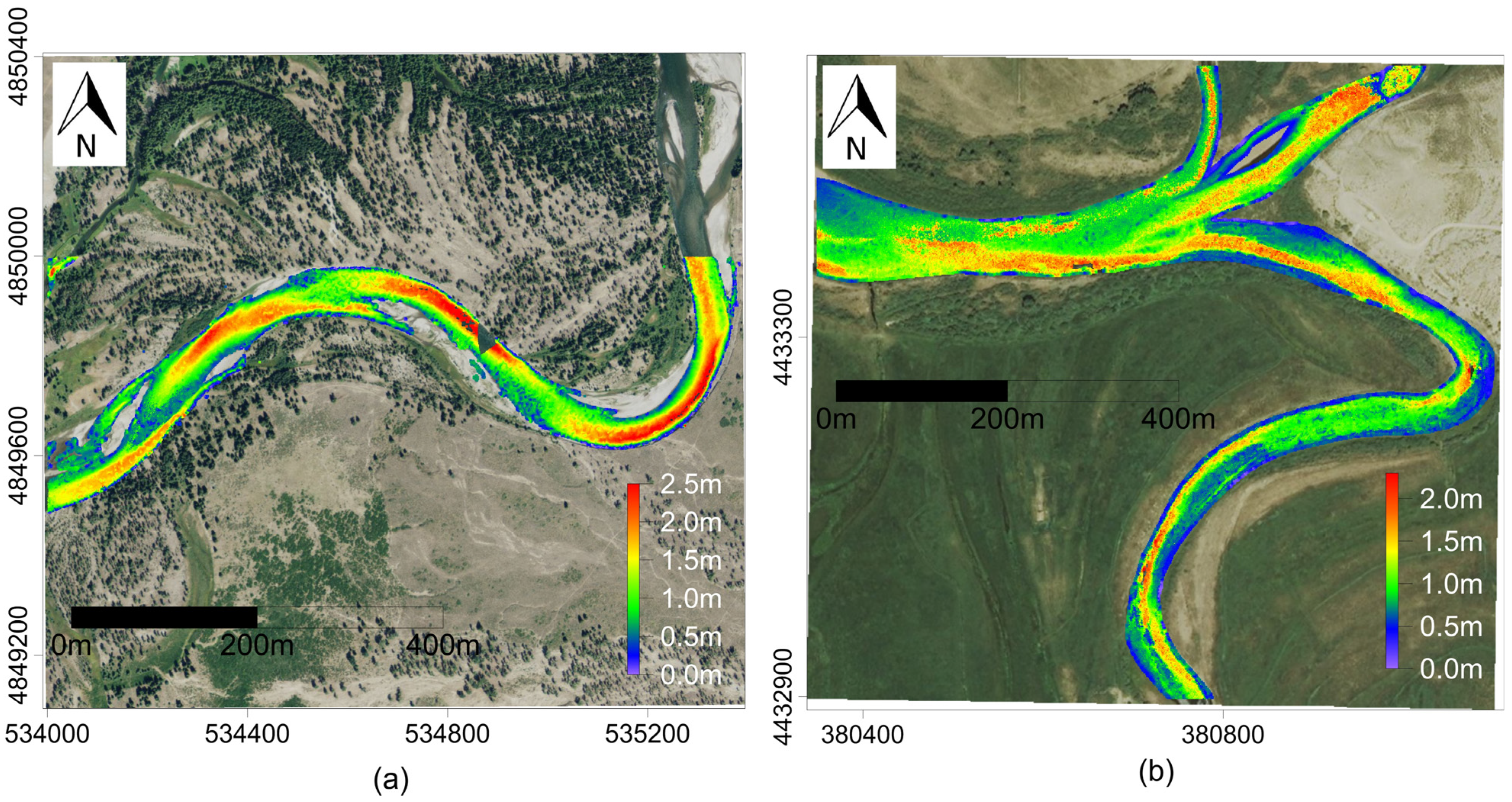
The objective of the study was to evaluate the performance of a single band full waveform bathymetric LiDAR with different processing algorithms and water surface definitions in two distinct fluvial environments. We proposed a novel full waveform processing algorithm based on a continuous waveform transformation; the detected peaks from CWT are used as candidate seed peaks for both Gaussian and ESR decomposition. The wavelet transformation was assessed in comparison with a more standard approach of using Gaussian decomposition with initial peak estimates from a second derivative analysis. Water depths from each waveform method, along with discrete points produced by the real-time constant fraction discriminator have been compared to field measured water depths. All the methods have been applied to two fluvial environments: the clear and shallow (mostly < 2 m) water of the Snake River, and the turbid and shallow (mostly < 1.5 m) fluvial environment of the Blue/Colorado River.
In a summary, full waveform processing can produce more points than discrete CFD processing to provide better coverage and more multiple returns for better discrimination of benthic returns from water surface returns. However, with all approaches it is difficult to acquire good quality data for turbid water, especially when the water is shallow. The proposed CWT method shows better stability through varying water clarity conditions than the Gaussian or ESR decomposition methods also tested. A single band full waveform bathymetric LiDAR does not appear to be as accurate as a two wavelengths system that recovers the water surface using a NIR laser. However, with an appropriate full waveform processing algorithm, the error in determining the water surface from a single band green LiDAR can be mitigated; these results are encouraging because they seem to indicate that with improved detection of the water surface from the green LiDAR we can expect a single band LiDAR bathymetry system to perform similarly to a two band (NIR and green) bathymetric system. For this to be realized, however, we must successfully extract the water surface from the relatively complex backscatter at the air/water interface, which we were unable to do with the waveform processing algorithms presented. In [
23], they proposed a quadrilateral signal to model the effect of water column scattering, and show it to be effective with simulated bathymetric LiDAR data. However, our initial analysis of this methodology has not shown a significant improvement in water surface estimation for the Aquarius datasets examined. Future work will therefore focus on decoupling the water surface and water column scattering at the air/water interface.


 ,
, 


