Spatial Feature Reconstruction of Cloud-Covered Areas in Daily MODIS Composites

Abstract

The opacity of clouds is the main problem for optical and thermal space-borne sensors, like the Moderate-Resolution Imaging Spectroradiometer (MODIS). Especially during polar nighttime, the low thermal contrast between clouds and the underlying snow/ice results in deficiencies of the MODIS cloud mask and affected products. There are different approaches to retrieve information about frequently cloud-covered areas, which often operate with large amounts of days aggregated into single composites for a long period of time. These approaches are well suited for static-nature, slow changing surface features (e.g., fast-ice extent). However, this is not applicable to fast-changing features, like sea-ice polynyas. Therefore, we developed a spatial feature reconstruction to derive information for cloud-covered sea-ice areas based on the surrounding days weighted directly proportional with their temporal proximity to the initial day of interest. Its performance is tested based on manually-screened and artificially cloud-covered case studies of MODIS-derived polynya area data for the polynya in the Brunt Ice Shelf region of Antarctica. On average, we are able to completely restore the artificially cloud-covered test areas with a spatial correlation of 0.83 and a mean absolute spatial deviation of 21%.

1. Introduction

Cloud cover is the crucial deficit of optical and thermal-infrared space-borne remote sensing compared to microwave systems. Satellite products, such as the Moderate-Resolution Imaging Spectroradiometer (MODIS) cloud mask (MOD35), which incorporates a total of 19 different spectral bands of passive-reflected and infrared radiation, show in general good results for polar daytime (e.g., [1,2]). However, their performance decreases drastically during polar nighttime (e.g., [1,3,4,5]). This results from the lack of visible channels in the analysis and testing, as well as the low thermal contrast between clouds and the underlying snow/ice [1,2,6].

Liu et al. [2] further improved the MODIS cloud mask especially for nighttime polar cloud detection. The addition of new tests and modifications showed drastic improvements in cloud detection for two Arctic stations and one Antarctic station. However, despite an overall improvement, the MODIS cloud mask still fails to detect very thin cloud cover and clouds during conditions of weak temperature inversions, where the surface temperature is below 250 K. While strong improvements were achieved, confident cloud cover detection in polar nighttime over snow and ice surfaces remains a problem [1].

Fraser et al. [7] introduced a compositing procedure of MODIS swaths from a customizable number of days in order to achieve information of Antarctic fast-ice areas. For such an application, this method is sufficient due to the static nature of fast ice and was successfully applied in a follow-up study [8]. However, in order to monitor or detect rather fast-changing features, such as polynyas, this method turned out to be unsatisfactory due to its necessary large compositing intervals.

Previous studies that investigated polynya dynamics based on MODIS-derived thin ice thickness data either did not correct their results for cloud-covered regions [9] or used a simple mathematical scheme of proportional extrapolation [10]. In the latter approach, polynya area (POLA) is assigned to cloud-covered areas in the same proportion as is detected in the cloud-free area. For example, if a region is 80% cloud-free and 50% of this area features a polynya signal, then 50% of the cloud-covered 20% is considered polynya area. However, polynyas are recurring areas of thin ice and open water that are generally formed by divergent ice motion (e.g., [11,12,13]) and, therefore, have a higher probability of occurrence in some regions than in others. With the approach used by Preußer et al. [10], polynya area gets potentially assigned to regions that are very unlikely to feature a polynya.

Accurate estimation of POLA is crucial for the investigation of sea-ice properties and air-ice-ocean interactions. Variations in polynya area influence, for example, the surface energy balance of sea ice and, thereby, alter the ocean/atmosphere heat and moisture exchange, as well as the rate of ice production and bottom water formation (e.g., [11,12,14,15,16]). POLA data are also used as boundary conditions in simulations with numerical models [17]. They can also be assimilated into sea-ice/ocean models.

In this study, we present a simple, yet robust, statistical approach to reconstruct cloud-covered surface features based on daily binary MODIS composites for adaptable time intervals. While the algorithm is generally applicable to comparable problems, we will describe and discuss its application and performance on the example of POLA time series with the focus on improving the monitoring of polynya dynamics (e.g., [9,10,18]).

2. Data and Methods

2.1. Input Data

In this study, we use thin-ice thickness (TIT) data to define POLA, which were derived from a combination of satellite imagery and atmospheric reanalysis data. The procedure, as well as all equations are thoroughly described in Adams et al. [9]. The thin-ice retrieval makes use of the ice-surface temperature dataset (IST) in the MODIS Sea Ice product (MOD/MYD29, [4,5]), distributed by the U.S. National Snow and Ice Data Center (NSIDC). The provided data has a spatial resolution of 1 km × 1 km at nadir, and each swath covers an area of 1354 km (across track) × 2030 km (along track), which equals approximately 5 min of satellite travel time. The overall IST accuracy of the MOD/MYD29 sea-ice product under ideal (i.e., clear-sky) conditions is 1–3 K [4,5]. The MOD/MYD29 data product was already corrected for cloud cover using the MODIS cloud mask.

The set of input data is complemented by the European Centre of Medium Range Weather Forecast (ECMWF) ERA-Interim Reanalysis data [19]. The ERA-Interim data are distributed at a spatial resolution of 0.75° and were linearly interpolated to spatially and temporarily fit the MODIS data. All MODIS swaths along with the ERA-Interim datasets were projected onto a common reference grid using a nearest neighbor approach. No interpolation was applied.

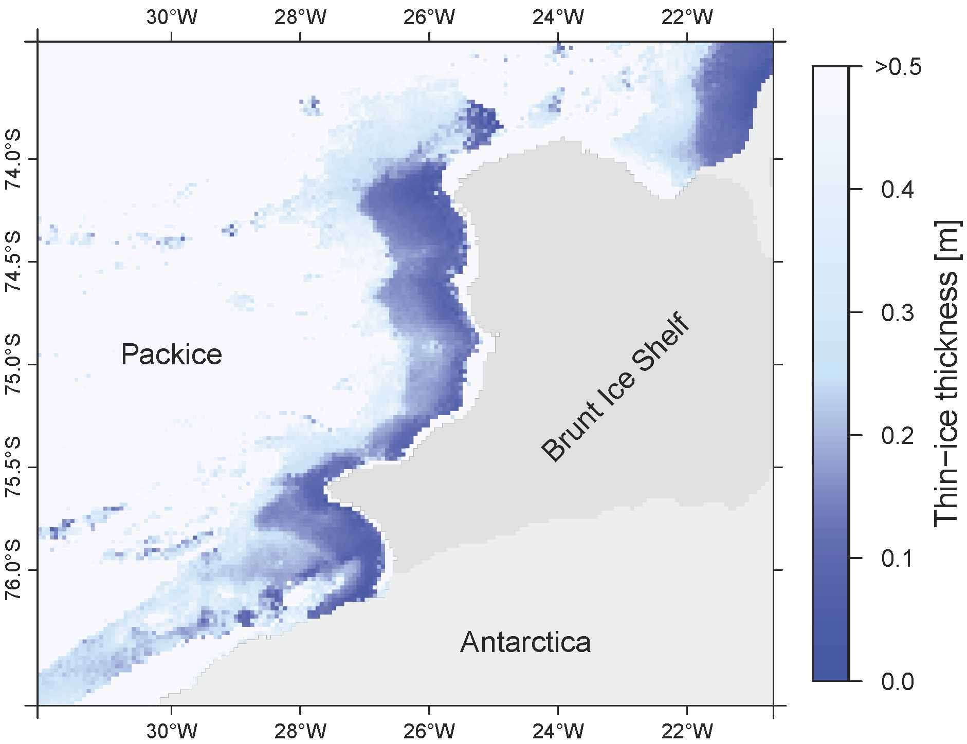
We apply the TIT-retrieval technique to all available MODIS IST swaths in a sub-region of the Southern Weddell Sea, namely the Brunt Ice Shelf region (Figure 1), for the austral winter (1 April to 30 September) of the years from 2002 to 2013. The Brunt Ice Shelf region is located from 20–31°W and 73.4–76.6°S, with a spatial extent of approximately 120,000 km². Subsequently, daily median-TIT composites are computed and binary POLA maps (BPM) are derived using a TIT threshold of 0.2 m [9]. For a maximum obtained ice thickness of 0.2 m, Adams et al. [9] state an uncertainty of ± 4.7 cm, while ice thickness measurements above a 0.2-m threshold yield significantly higher uncertainties. Therefore, we limit our investigation accordingly. A threshold of 0.2 m is also used by sea-ice model studies to define the polynya area [14].

Figure 1. Area of investigation in the Southern Weddell Sea around the Brunt Ice Shelf with example MOD/MYD29-derived thin ice thickness composite (6 September 2012) highlighting the most active polynya areas in the Brunt Ice Shelf region.

Figure 1. Area of investigation in the Southern Weddell Sea around the Brunt Ice Shelf with example MOD/MYD29-derived thin ice thickness composite (6 September 2012) highlighting the most active polynya areas in the Brunt Ice Shelf region.

In this study, we focus on the reconstruction of data gaps in the daily composites, which result from detected cloud cover by the MODIS cloud mask. Additionally, we artificially introduce clouds to daily composites in several case studies to set up and evaluate the approach.

2.2. Spatial Feature Reconstruction Algorithm

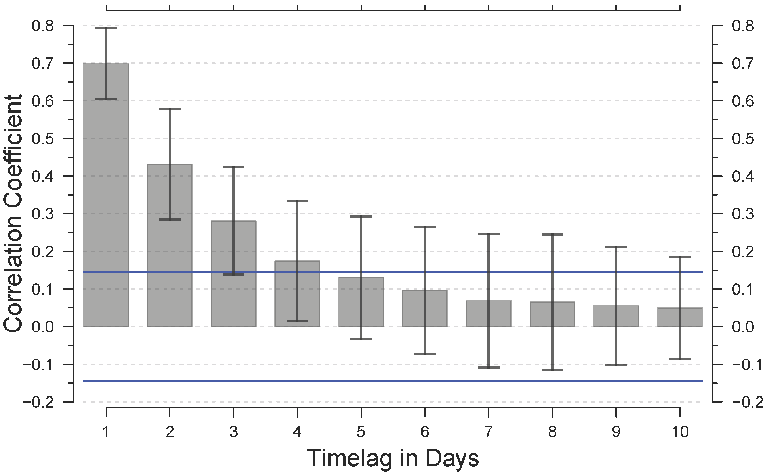
Polynya activity varies on a short time scale, specifically in the coastal regions of the Southern Weddell Sea, as can be seen from the auto-correlation function (ACF, Figure 2) of POLA time series from the Brunt Ice Shelf region. Hence, a gap-filling approach for daily POLA maps based on MODIS composites requires a technique that aims at daily resolution, which makes the method as described by Fraser et al. [7] not applicable here.

On average, a 3-day time lag in each year still shows a significant correlation to the initial polynya signal (average ±1 standard deviation; Figure 2). However, this correlation drops quickly with increasing temporal distance, i.e., the similarity in polynya size and shape between days decreases with increasing temporal distance. Additionally, the per-pixel gap length resulting from cloud coverage is in most instances equal to or below three consecutive days (91.79% of the total frequency distribution), with a majority on 1-day (57.83%) and 2-day (23.62%) gaps.

Figure 2. Auto-correlation function based on the MODIS-derived polynya area in the Brunt Ice Shelf region (Figure 1) from 1 April to 30 September for the years 2002 to 2013. Presented in gray bars are the auto-correlation coefficients against the absolute time lag in days, i.e., a negative, as well as a positive displacement. Values above the blue line indicate a significant correlation, given a level of significance (α) of 5%. Error bars indicate ±1 standard deviation.

Figure 2. Auto-correlation function based on the MODIS-derived polynya area in the Brunt Ice Shelf region (Figure 1) from 1 April to 30 September for the years 2002 to 2013. Presented in gray bars are the auto-correlation coefficients against the absolute time lag in days, i.e., a negative, as well as a positive displacement. Values above the blue line indicate a significant correlation, given a level of significance (α) of 5%. Error bars indicate ±1 standard deviation.

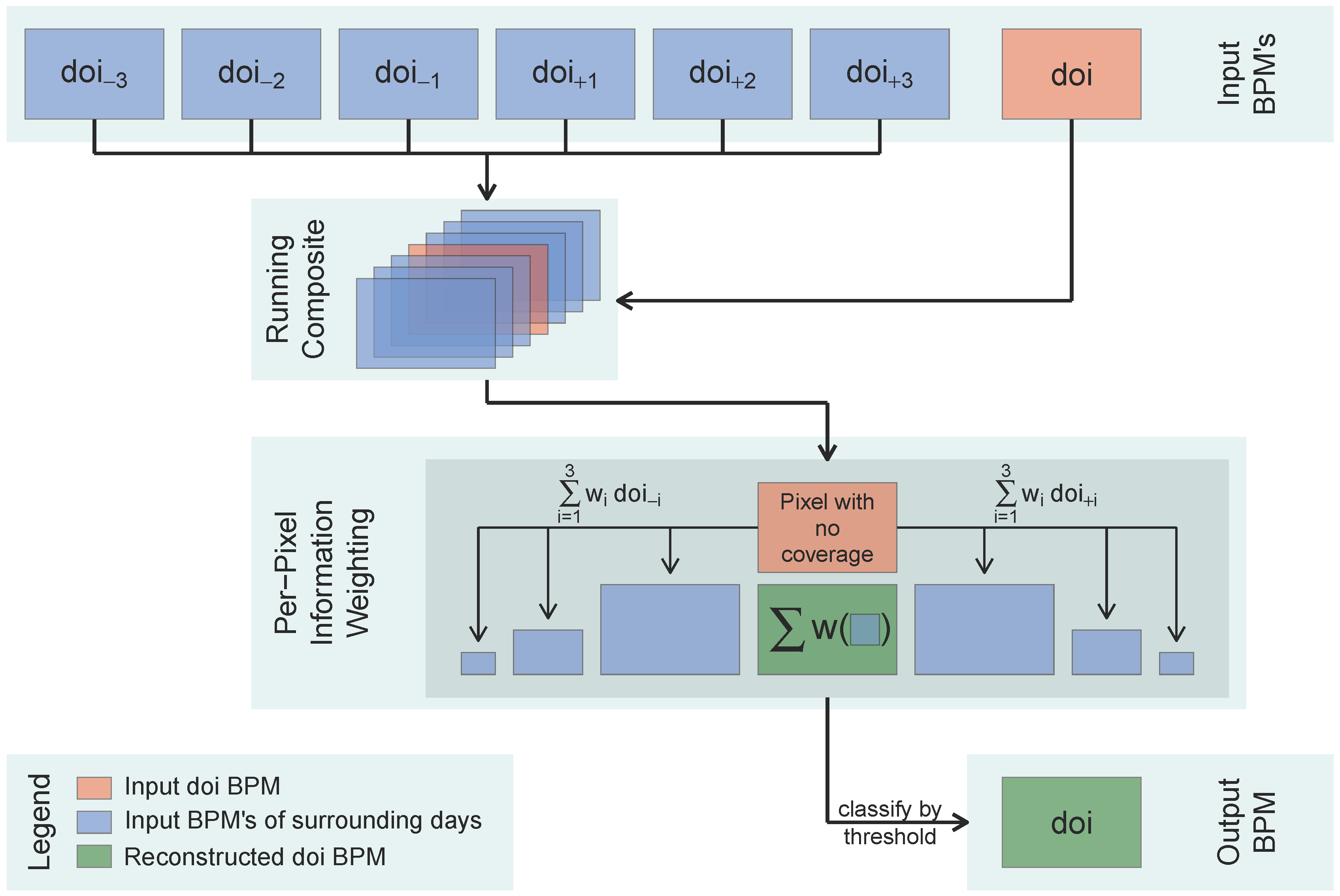
Our approach aggregates daily BPMs of a fixed number of days surrounding an initial day of interest (doi; Figure 3). The length of the applied time interval is variable and depends on the type and change-rate of the investigated surface feature. In our case of coastal polynyas, we decided to use a ±3 day time interval. This was based on the fact that the POLA information is on average significantly correlated within at least three days (Figure 2) and that >90% of gaps are shorter than four days. By weighting the aggregated information on polynya activity in those six surrounding days (doi₋₃...doi₊₃) based on their temporal proximity, an inference of the cloud-covered areas can be derived for the center day of interest (doi).

Figure 3. Flow chart of the general algorithm procedure. Binary polynya area maps (BPM) of the surrounding days (doi₋₃...doi₊₃, blue) are aggregated and weighted according to their temporal proximity to the day of interest (doi, red). By passing a predefined threshold, each cloud-covered pixel in the initial day of interest is classified as polynya area or thick ice, resulting in a reconstructed BPM of the initial day of interest (green).

Figure 3. Flow chart of the general algorithm procedure. Binary polynya area maps (BPM) of the surrounding days (doi₋₃...doi₊₃, blue) are aggregated and weighted according to their temporal proximity to the day of interest (doi, red). By passing a predefined threshold, each cloud-covered pixel in the initial day of interest is classified as polynya area or thick ice, resulting in a reconstructed BPM of the initial day of interest (green).

$$WF{R}_{6d}={\displaystyle \sum _{j=1}^3}{w}_j(do{i}_j+do{i}_{-j})$$

(1)

This procedure of a weighted feature reconstruction (WFR) is summarized in Equation (1) for the case of a ±3-day time interval (WFR_6d). Here, w_j are the daily weighting factors and doi_−j and doi_j are the daily BPMs surrounding the initial day of interest that needs to be reconstructed due to the presence of clouds (Figure 3). However, the application is bound to some necessary constraints to better explain the algorithm:

• The total sum of all weighting factors should add up to one, which yields a probability for each pixel to be POLA.

• The weighting factors are mirrored corresponding to their temporal distance to the initial day of interest, i.e., the same weighting factor w₂ is assigned to the BPMs of doi₋₂ and doi₊₂. The mirrored setup is in accordance with the results of the auto-correlation function, showing a significant correlation with positive, as well as negative temporal displacement.

• Weights increase with increasing temporal proximity to the initial day of interest on the basis of Figure 2.

We artificially introduce cloud cover into BPMs (i.e., we set the present POLA to zero) in order to investigate the potential to properly restore the known polynya signal of the day of interest from the surrounding days. We chose two investigation approaches by either introducing cloud cover to the complete day of interest BPM or by just covering three spatially constant areas that comprise approximately 50% of the sea-ice area with artificial clouds. However, an assessment following this idea strongly depends on the amount and quality of the selected case studies. These case studies preferably comprise a large amount of clear-sky input BPMs.

In total, we chose a selection of 66 7-day long manually-screened case studies in the Brunt Ice Shelf region from the years 2002 to 2013. Out of those 66, 10 case studies feature almost constantly present clear-sky conditions over the majority of the 7-day time interval. The remaining 56 case studies also feature cloud-covered days in the 7-day time interval, which presumably is closer to reality in terms of general cloud and weather conditions. The spatial correlation coefficient of POLA (based on a Spearman pairwise correlation) of each surrounding day to the POLA of the initial day of interest, i.e., the day in the center of the 7-day time interval, for each of the ten clear-sky case studies is shown in Table 1. From the high variability in correlation coefficients, it becomes clear that there is a high daily variability in POLA, which is due to the prevailing polynya dynamics.

Table 1. Summary of the spatial correlation coefficients between the polynya area of the initial day of interest (doi) and the polynya area of the surrounding days (doi₋₃ ... doi₊₃) for the ten constant clear-sky case studies. Numbers in parenthesis indicate the percentage cloud-covered fraction (%) in the respective daily MODIS composite.

Case	doi−3	doi−2	doi−1	doi+1	doi+2	doi+3
1	0.69 (7)	0.82 (11)	0.91 (13)	0.91 (13)	0.76 (15)	0.10 (8)
2	0.77 (13)	0.53 (5)	0.88 (14)	0.82 (17)	0.58 (13)	0.18 (1)
3	0.81 (21)	0.81 (23)	0.87 (21)	0.87 (21)	0.79 (20)	0.46 (7)
4	0.65 (15)	0.68 (33)	0.81 (21)	0.80 (30)	0.71 (15)	0.69 (19)
5	0.66 (52)	0.62 (40)	0.86 (37)	0.76 (30)	0.68 (32)	0.46 (14)
6	0.32 (2)	0.88 (14)	0.90 (14)	0.85 (13)	0.82 (13)	0.80 (19)
7	0.72 (14)	0.77 (19)	0.88 (17)	0.60 (7)	0.41 (5)	0.03 (2)
8	0.74 (16)	0.76 (16)	0.90 (13)	0.79 (9)	0.50 (4)	0.35 (3)
9	0.43 (6)	0.56 (10)	0.91 (24)	0.91 (27)	0.78 (23)	0.28 (3)
10	0.19 (1)	0.73 (13)	0.85 (20)	0.90 (19)	0.71 (13)	0.50 (9)

Table 1. Summary of the spatial correlation coefficients between the polynya area of the initial day of interest (doi) and the polynya area of the surrounding days (doi₋₃ ... doi₊₃) for the ten constant clear-sky case studies. Numbers in parenthesis indicate the percentage cloud-covered fraction (%) in the respective daily MODIS composite.

Case	doi−3	doi−2	doi−1	doi+1	doi+2	doi+3
1	0.69 (7)	0.82 (11)	0.91 (13)	0.91 (13)	0.76 (15)	0.10 (8)
2	0.77 (13)	0.53 (5)	0.88 (14)	0.82 (17)	0.58 (13)	0.18 (1)
3	0.81 (21)	0.81 (23)	0.87 (21)	0.87 (21)	0.79 (20)	0.46 (7)
4	0.65 (15)	0.68 (33)	0.81 (21)	0.80 (30)	0.71 (15)	0.69 (19)
5	0.66 (52)	0.62 (40)	0.86 (37)	0.76 (30)	0.68 (32)	0.46 (14)
6	0.32 (2)	0.88 (14)	0.90 (14)	0.85 (13)	0.82 (13)	0.80 (19)
7	0.72 (14)	0.77 (19)	0.88 (17)	0.60 (7)	0.41 (5)	0.03 (2)
8	0.74 (16)	0.76 (16)	0.90 (13)	0.79 (9)	0.50 (4)	0.35 (3)
9	0.43 (6)	0.56 (10)	0.91 (24)	0.91 (27)	0.78 (23)	0.28 (3)
10	0.19 (1)	0.73 (13)	0.85 (20)	0.90 (19)	0.71 (13)	0.50 (9)

Applying different weights (w_j ; Equation (1)) permits control over the necessary amount of available POLA information and their temporal position relative to the center day of interest for a pixel to be classified as POLA, given a predefined POLA probability threshold (th). In order to optimize the combination of weighting factors and threshold, i.e., to calibrate the approach, the method is evaluated based on two statistical measures:

• A summarized spatial root-mean-squared error (RMSE) that represents the total POLA difference.

• The degree of spatial correlation (R) between actual POLA and restored data based on a Spearman pairwise correlation coefficient.

In order to find the best combination of weighting factors and POLA probability threshold, we chose to iteratively minimize the RMSE and maximize the spatial correlation (R) between actual POLA (i.e., the POLA of the BPM of the initial day of interest) and reconstructed POLA (i.e., the resulting BPM of the WFR approach). The iterative procedure starts with a predefined set of weighting factors and threshold (e.g., w₃ = 0.01, w₂ = 0.02, w₁ = 0.47 and th = 0.01) that are in agreement with the previously-defined restrictions. In this setup, the sum of all weighting factors for the six surrounding days is equal to 1; weights increase with temporal proximity to the initial day of interest and are mirrored for equal temporal distance. In order to minimize computation time, the threshold value can only adopt values of possible weighting factor summations. For each set of weighting factors and threshold, the RMSE and the mean spatial POLA correlation for all available case studies were calculated. Weighting factors are then modified in steps of 0.01, e.g., to w₃ = 0.01, w₂ = 0.03, w₁ = 0.46 and th = 0.01. Subsequently, RMSE and R were calculated for each threshold again. We did these calculations for all possible weighting factors and threshold combinations and for both datasets of 66 and 10 case studies.

In order to highlight the advantage of our WFR_6d procedure, we calculated RMSE and R also for three reference runs comprising a ±2 weighted time interval (WFR_4d), as well as for an equally-weighted reconstruction (EWR) based on a ±3-day time interval (EWR_6d) and a ±1-day (EWR_2d) time interval. WFR_6d and EWR_6d are then applied to a five-year period of POLA data in the Brunt Ice Shelf region (1 April to 30 September 2006–2010), to compare estimates of unaccounted POLA due to detected cloud cover.

3. Results

3.1. Evaluation of Weights/Threshold Combinations

While a number of combinations showed good results in a small range of R and RMSE, three combinations of daily weighting factors and threshold achieved the best overall result and were chosen for further investigation and comparison (Table 2):

• Based on the complete 66 case study dataset, two combinations showed best results in minimum RMSE and high spatial POLA correlation. Combination 1 (CMB1, w₃ = 0.02, w₂ = 0.16, w₁ = 0.32 and th = 0.34) showed the second smallest RMSE, as well as the largest spatial correlation (R).

• Combination 2 (CMB2, w₃ = 0.04, w₂ = 0.14, w₁ = 0.32 and th = 0.36) showed the smallest RMSE along side the largest spatial correlation (R) for the complete 66 case study dataset.

• For the subset case study dataset, Combination 3 (CMB3, w₃ = 0.01, w₂ = 0.05, w₁ = 0.44 and th = 0.46) showed the smallest RMSE.

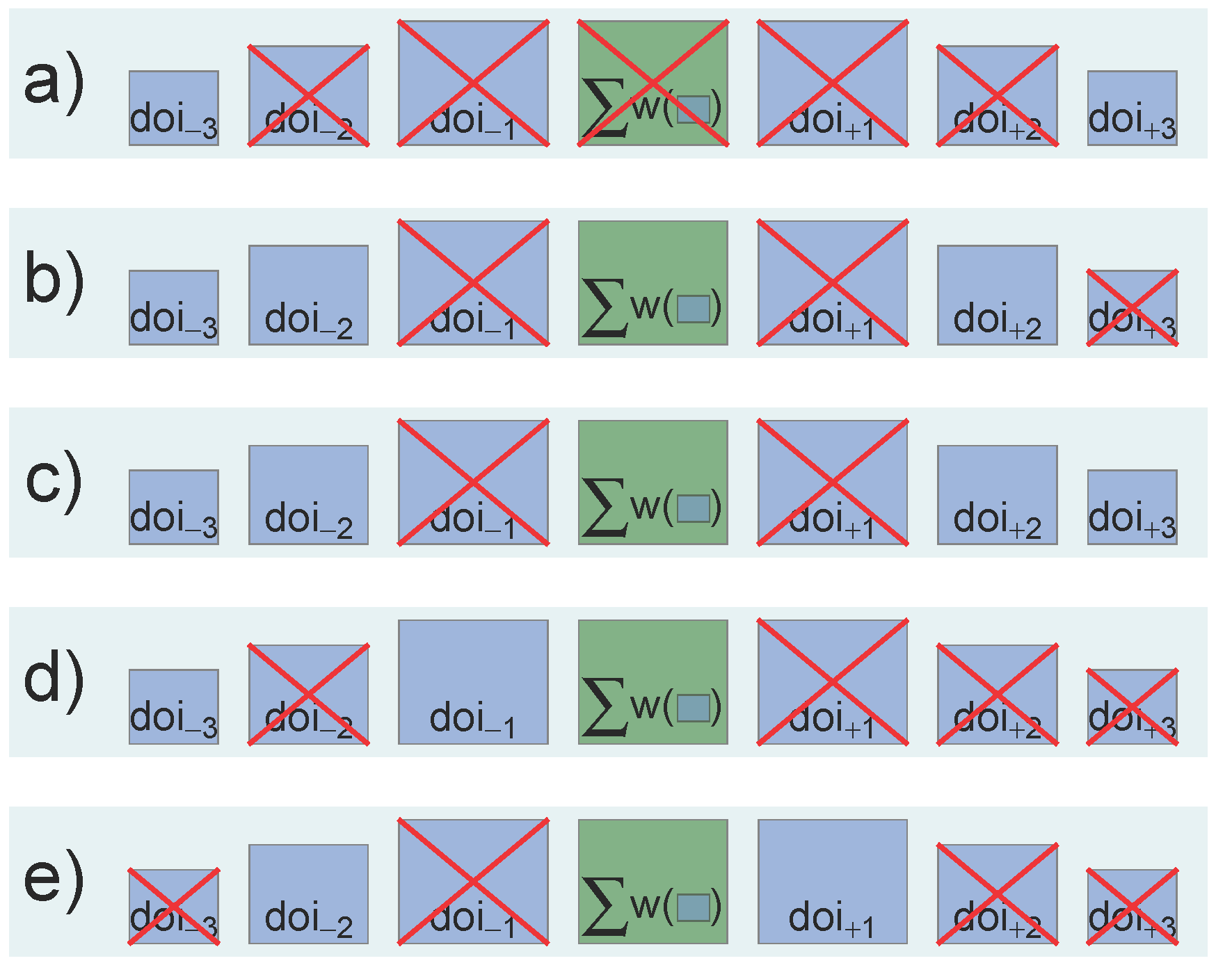
When elaborating on CMB1 and CMB2 and why we chose to investigate and use both combinations, the difference comes down to the necessary amount of covered surrounding days that feature a polynya signal, for the WFR approach to classify a cloud-covered pixel in the initial day of interest as POLA. This necessary amount of available POLA information and their temporal position relative to the center day of interest is different for each of the three combinations. An explanation is presented in Figure 4:

• A gap of five consecutive days (i.e., only the outer days contain cloud-free information for the WFR_6d composite) will not result in the classification of that pixel as POLA for either of the three combinations (Figure 4a).

• Gaps of three consecutive days (i.e., cloud-free information from both inner days is unavailable for the WFR_6d composite; Figure 4b,c) may result in the classification of that pixel as POLA, depending on the combination. The example in Figure 4b will not result in a POLA classification for CMB2 and CMB3. However, the Figure 4c example will be classified as POLA using either CMB1 or CMB2.

• For gaps of two consecutive days (i.e., cloud-free information from one inner day is unavailable for the WFR_6d composite; Figure 4d,e), any additional spatial information of one other day will result in the classification of that pixel as POLA for each of the three combinations.

Table 2. Summary of resulting statistics of the spatial root-mean-squared error (RMSE, km²) and spatial correlation coefficient (R) of polynya area for the complete set of 66 case studies (RMSE₆₆/R₆₆) and a 10-day subset of almost constant clear-sky conditions (RMSE₁₀/R₁₀). Results are shown for the weighted ±3-day time interval WFR_6d (weighted feature reconstruction (WFR)) based on our three “best fit” combinations (CMB1-CMB3) and three comparison runs comprising the weighted ±2-day time interval (WFR_4d), as well as equally-weighted reconstruction runs based on a ±3- and a ±1-day time interval (EWR_6d and EWR_2d). EWR_6d is shown based on a minimum threshold of two (M2) or three days (M3) with polynya area (POLA). Numbers in parenthesis indicate the reconstruction results for an only partially-introduced cloud cover (about 50% of the sea-ice area).

	WFR6d-CMB1	WFR6d-CMB2	WFR6d-CMB3	EWR6d-M2	EWR6d-M3	WFR4d	EWR2d
RMSE66	1904 (1285)	1902 (1285)	1988 (1321)	2079 (1386)	2855 (1827)	1988 (1321)	2267 (1556)
RMSE10	859 (705)	858 (704)	812 (683)	1907 (1058)	1355 (795)	812 (683)	1467 (992)
R66	0.83 (0.85)	0.83 (0.85)	0.82 (0.84)	0.80 (0.83)	0.75 (0.77)	0.82 (0.84)	0.79 (0.81)
R10	0.92 (0.93)	0.92 (0.93)	0.91 (0.93)	0.88 (0.90)	0.88 (0.91)	0.91 (0.93)	0.89 (0.91)

Table 2. Summary of resulting statistics of the spatial root-mean-squared error (RMSE, km²) and spatial correlation coefficient (R) of polynya area for the complete set of 66 case studies (RMSE₆₆/R₆₆) and a 10-day subset of almost constant clear-sky conditions (RMSE₁₀/R₁₀). Results are shown for the weighted ±3-day time interval WFR_6d (weighted feature reconstruction (WFR)) based on our three “best fit” combinations (CMB1-CMB3) and three comparison runs comprising the weighted ±2-day time interval (WFR_4d), as well as equally-weighted reconstruction runs based on a ±3- and a ±1-day time interval (EWR_6d and EWR_2d). EWR_6d is shown based on a minimum threshold of two (M2) or three days (M3) with polynya area (POLA). Numbers in parenthesis indicate the reconstruction results for an only partially-introduced cloud cover (about 50% of the sea-ice area).

	WFR6d-CMB1	WFR6d-CMB2	WFR6d-CMB3	EWR6d-M2	EWR6d-M3	WFR4d	EWR2d
RMSE66	1904 (1285)	1902 (1285)	1988 (1321)	2079 (1386)	2855 (1827)	1988 (1321)	2267 (1556)
RMSE10	859 (705)	858 (704)	812 (683)	1907 (1058)	1355 (795)	812 (683)	1467 (992)
R66	0.83 (0.85)	0.83 (0.85)	0.82 (0.84)	0.80 (0.83)	0.75 (0.77)	0.82 (0.84)	0.79 (0.81)
R10	0.92 (0.93)	0.92 (0.93)	0.91 (0.93)	0.88 (0.90)	0.88 (0.91)	0.91 (0.93)	0.89 (0.91)

Figure 4. Summary of different combinations of necessary daily binary POLA maps for a cloud-covered pixel (green) to be classified as POLA. This is based on WFR_6d-CMB1 with w₃ = 0.02, w₂ = 0.16, w₁ = 0.32 and th = 0.34. Colors correspond to Figure 3. Crossed out boxes symbolize missing data (blue boxes) or a classification as non-POLA (green box).

Figure 4. Summary of different combinations of necessary daily binary POLA maps for a cloud-covered pixel (green) to be classified as POLA. This is based on WFR_6d-CMB1 with w₃ = 0.02, w₂ = 0.16, w₁ = 0.32 and th = 0.34. Colors correspond to Figure 3. Crossed out boxes symbolize missing data (blue boxes) or a classification as non-POLA (green box).

All of these examples were made under the assumption that each of the available pixels shows a POLA signal. Otherwise, the assigned daily weights of those pixels will not be added to the WFR_6d approach. This is the same for pixels in the surrounding days that are covered by clouds. Both pixel states, not featuring a polynya signal or being cloud covered, decrease the likelihood for the day of interest pixel to be classified as POLA.

3.2. Comparison Based on R and RMSE

In Table 2, the results of RMSE and R are presented for the WFR_6d approach (based on CMB1, CMB2 and CMB3) and the four reference runs based on a shorter time interval (WFR_4d) and without applying the weighting scheme (EWR_6d-M2, EWR_6d-M3, EWR_2d). The WFR approaches generally achieve the best results of minimum RMSE and maximum spatial correlation (R), when compared to the EWR reference runs. However, the differences are relatively small. While the ±2 and ±1 reference runs (WFR_4d and EWR_2d) achieve good results, their application is limited to two-day and one-day gaps in the data. While this is also true for WFR_6d-CMB3, the results of the ±3-day approach are slightly better. However, the initial situation in the 10 case study sample size cannot be considered representative for the general cloud situation in the Brunt Ice Shelf region. These results underline also the importance of the kernel edges (doi_±3), which allow covering larger gaps despite their small weighting factors. The WFR_6d results vary only for the RMSE results and show consistent results for the spatial correlation (R). For the equal weight reconstruction approach (EWR_6d), the best result for the 66 case study dataset was achieved when a pixel is classified as POLA, when at least two out of the six input days contain a POLA signal (EWR_6d-M2). For the clear-sky subset of 10 case studies, EWR_6d shows the best result when based on a minimum of three days with POLA signal (EWR_6d-M3).

We draw the same conclusions by investigating only partially cloud-covered day of interest BPMs (Table 2, numbers in parenthesis), only with overall better results. Considering the average auto-correlation (Figure 2) and the gap-length distribution, we focus on the use of WFR_6d-CMB1 and WFR_6d-CMB2, as both combinations are applicable to three-day coverage gaps. In general, although both statistics (RMSE and R) are important, we consider the spatial correlation more accurate and important. This is due to the fact that the stated RMSE value is without any spatial reference, i.e., the summarized spatial extent might be accurate, but its per-pixel distribution in the BPM can be incorrect.

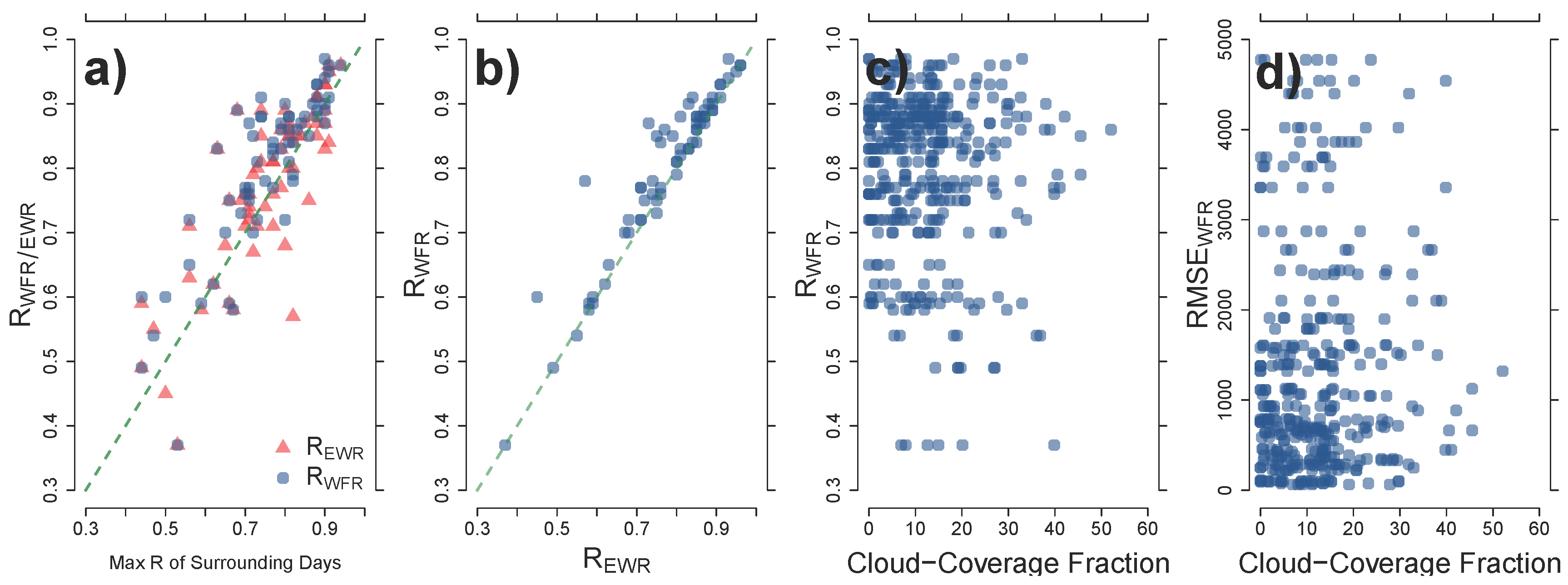
The summarized results of the 66 case studies between WFR_6d-CMB1 and EWR_6d-M2 are shown in Figure 5. In Figure 5a, the resulting spatial correlation coefficients of POLA between WFR_6d and EWR_6d and the initial day of interest (R_WFR and R_EWR) are plotted against the maximum correlation coefficients of the respective surrounding days (Table 1). The WFR_6d-CMB1 approach yields in 48 cases a higher spatial correlation to the initial day of interest than any of the surrounding days. In 11 cases, the spatial correlation is lower than the maximum of the surrounding days, and it is equal in seven cases. For the EWR_6d-M2 approach, only 43 cases show a higher spatial correlation, while 22 cases show a lower spatial correlation than the maximum of the surrounding days. The spatial correlation is equal for only one case.

Figure 5. Summary of differences between weighted WFR_6d-CMB1 and equally-weighted EWR_6d-M2 approaches. (a) Scatterplot of the resulting spatial correlation coefficients R_WFR and R_EWR with the day of interest against the maximum spatial correlation of any of the six surrounding days with the initial day of interest. (b) Scatterplot of R_WFR against R_EWR. (c,d) Scatterplots of WFR_6d-CMB1 achieved R and RMSE against the present cloud coverage in the surrounding six days.

Figure 5. Summary of differences between weighted WFR_6d-CMB1 and equally-weighted EWR_6d-M2 approaches. (a) Scatterplot of the resulting spatial correlation coefficients R_WFR and R_EWR with the day of interest against the maximum spatial correlation of any of the six surrounding days with the initial day of interest. (b) Scatterplot of R_WFR against R_EWR. (c,d) Scatterplots of WFR_6d-CMB1 achieved R and RMSE against the present cloud coverage in the surrounding six days.

On average, based on a two-sided t-test, the combined information of several days is significantly better (α = 5%) compared to just mirroring the best correlated single day for the WFR approach. The EWR approach does not achieve a significant improvement.

In Figure 5b, the spatial correlation coefficients (R_WFR and R_EWR) are plotted against each other. Here, the WFR_6d-CMB1 approach shows slightly better (45 cases) or equal (17 cases) results. The EWR_6d-M2 approach is only superior in four cases. This highlights the overall potential of a weighted approach over a non-weighted approach to reconstruct polynya signals from the surrounding days due to the high change rate of polynya dynamics (Figure 2).

The effect of cloud cover in the surrounding six days on the results of spatial POLA correlation and RMSE is shown in Figure 5c,d, respectively. A clear clustering for both metrics is present in our data, where low amounts of present cloud cover improve the results by means of minimized RMSE and maximized spatial correlation in POLA. However, there are also exceptions where good results can be achieved even with relatively high amounts of present cloud cover in some of the surrounding days. On the other side, low amounts of cloud cover do not necessarily lead to optimal results. This might have several reasons. For example, naturally-induced high polynya dynamics in between days (e.g., by a change in the prevailing wind direction or general weather conditions) can of course decrease the spatial correlation and increase the difference in spatial extent in the reconstruction. However, also already mentioned errors in the classification of pixels due to deficiencies in the MODIS cloud mask may potentially play a role.

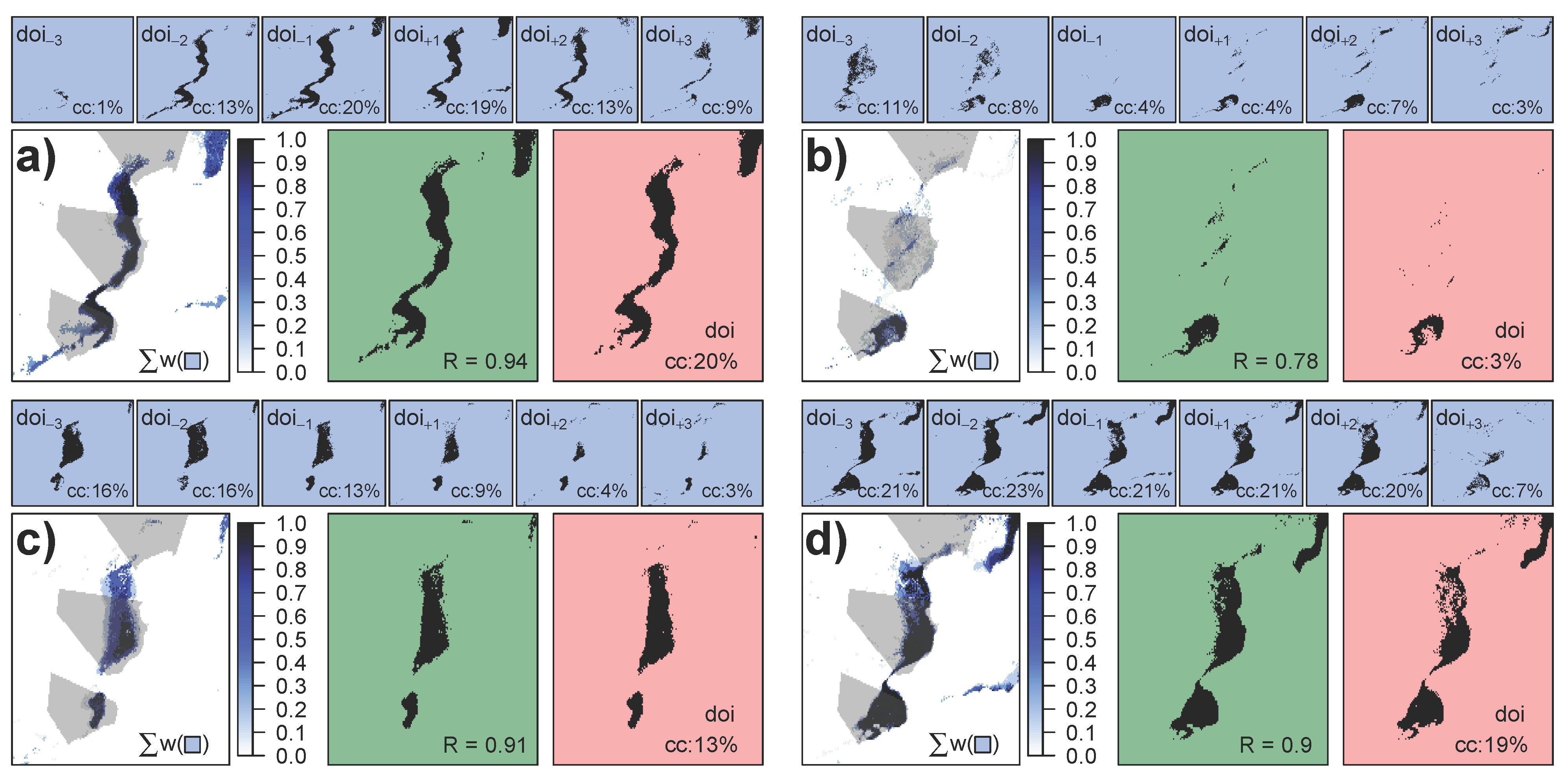
A set of four example case studies (Figure 6) highlights some additional aspects of the WFR_6d-CMB1 approach based on POLA investigations near the Brunt Ice Shelf. As shown in Figure 1, the main polynya activity near the Brunt Ice shelf is a narrow north-south/northeast-southwest strip along the ice-shelf edge. In Figure 6a, the initial polynya situation represents an almost complete cycle of polynya activity from opening to closing. The reconstruction corresponds closely to the initial BPM, showing a spatial correlation of 0.94 and a spatial difference of only 75 km². Figure 5b features an outlier where the resulting spatial correlation between the WFR_6d-CMB1 approach and the initial day of interest was significantly better than the EWR_6d-M2 reference run (0.78 to 0.57). Especially the center part, which is widely present in the BPMs of doi₋₃ and doi₋₂, will impair the EWR_6d-M2 reconstruction. A polynya closing event is featured in Figure 6c, where the POLA constantly decreases over the course of our seven-day interval. This is one example, where the EWR_6d reference run yields a large difference in POLA (1504 km² compared to 96 km² with WFR_6d-CMB1), due to the large extent of thin ice during doi₋₃ and doi₋₂. Especially opening and closing events are considered a primary reason for presumably large differences in average added POLA between WFR_6d and EWR_6d. Finally, Figure 6d shows a seven-day long (or longer) polynya event, but with varying POLA. The main difference is placed in the center region, where most of the surrounding days feature a strong polynya signal.

Figure 6. Set of four example case studies comprising binary POLA maps (BPM) surrounding the initial day of interest (blue), BPM of the initial day of interest (red), the WFR_6d-CMB1 composite and its derived BPM (green), as well as the spatial correlation (R) between derived BPM and actual BPM of the initial day of interest. Additionally, the percentage amount of present cloud cover (cc) is stated for each BPM. Gray areas highlight the partially artificially cloud-covered areas. Colors correspond to Figure 3; the geographic region corresponds to Figure 1. (a) Case Study 10 of Table 1; (b) one of the two major outlier examples in Figure 5b; (c) Case Study 8 of Table 1; and (d) Case Study 3 of Table 1.

Figure 6. Set of four example case studies comprising binary POLA maps (BPM) surrounding the initial day of interest (blue), BPM of the initial day of interest (red), the WFR_6d-CMB1 composite and its derived BPM (green), as well as the spatial correlation (R) between derived BPM and actual BPM of the initial day of interest. Additionally, the percentage amount of present cloud cover (cc) is stated for each BPM. Gray areas highlight the partially artificially cloud-covered areas. Colors correspond to Figure 3; the geographic region corresponds to Figure 1. (a) Case Study 10 of Table 1; (b) one of the two major outlier examples in Figure 5b; (c) Case Study 8 of Table 1; and (d) Case Study 3 of Table 1.

3.3. Application to POLA Time Series

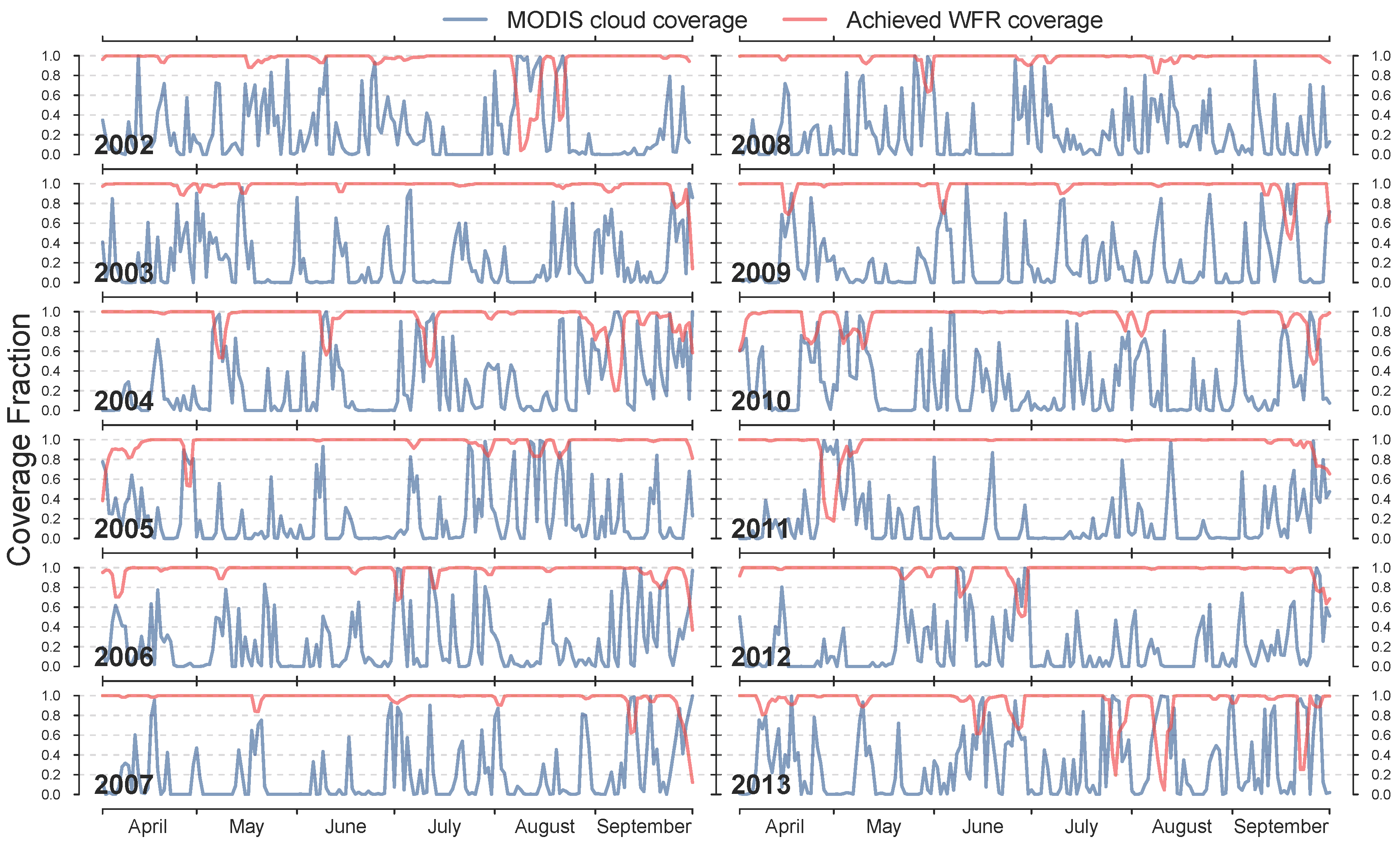
Differences between WFR_6d and EWR_6d by means of average spatial POLA correlation (R) and RMSE are not statistically significant (Table 2). When applying both procedures in their intended way to account for cloud-covered areas in the initial day of interest by utilizing the surrounding days, large and also statistically significant differences arise. On average, the Brunt Ice Shelf region features an average seasonal POLA of 9096 km² between 1 April and 30 September for the years 2006 to 2010. This value is based on the uncorrected MODIS-derived POLA time series used in this study. Therefore, the presented average most likely underestimates the true average POLA due to present cloud cover (Figure 7). On average, 22% of the area around the Brunt Ice Shelf (Figure 1) is cloud covered on each day between 2002 and 2013, as well as between 2006 and 2010. After application of the here presented WFR approach (in the WFR_6d-CMB1 setup), an average coverage of 96% and 97% was achieved per day for the time interval of 2002–2013 and 2006–2010, respectively.

Figure 7. Present MODIS cloud coverage for the Brunt Ice Shelf region (blue line) and the maximum achieved coverage using WFR_6d-CMB1 (red line) in decimal cover fraction.

Figure 7. Present MODIS cloud coverage for the Brunt Ice Shelf region (blue line) and the maximum achieved coverage using WFR_6d-CMB1 (red line) in decimal cover fraction.

The WFR_6d-CMB1 approach adds an average of 2433 km² of potentially missed POLA due to cloud-affected pixels. Results for the WFR_6d-CMB2 and WFR_6d-CMB3 are slightly lower due to the stricter threshold with 1852 km² and 1811 km², respectively. Additionally, WFR_6d-CMB2 and WFR_6d-CMB3 estimates are likely to be lower, because they were applicable in fewer cases than WFR_6d-CMB1. This was already mentioned for WFR_6d-CMB3, but is also true for WFR_6d-CMB2. On the other hand, the EWR_6d-M2 approach adds a seasonal average of 5047 km², which is believed to be too high by more than doubling the average POLA and given the aforementioned analysis. Based on the EWR_6d-M3 approach, an average of only 1058 km² will be added. These numbers were computed based on the raw BPMs without taking the newly added POLA information on previous days into account.

4. Discussion

Resulting from the deficiencies of the MODIS cloud mask, an existing cloud in any given pixel might be misclassified as sea ice. This misclassification results in a false ice thickness retrieval of either potential thin ice from a warm and low cloud or thick ice from a cold and high cloud. Both types of cloud artifacts deteriorate the resulting daily composite by adding false POLA to regions of pack ice or by altering the derived daily median TIT. However, these classification problems are not easily captured nor quantified without a large amount of in situ data and would therefore go beyond the scope of this study. A potential example is shown in Figure 6d, where less thin ice is shown in the center region of the day of interest compared to most of the surrounding days. This might be attributed to polynya dynamics or, despite great effort, to a poor case study selection for clear-sky conditions. However, it might also be a potential misclassification of clouds as thick ice, which was not detected by the MODIS cloud mask. These mentioned artifacts are likely to be present in many daily composites and, therefore, presumably reduce the results in spatial correlation in this study.

In general, the WFR approach can be applied to different time series datasets that need cloud-cover compensation on a daily resolution in contrast to, e.g., the method presented by Fraser et al. [8]. Adaptations have to be made based on the auto-correlation function of the dataset under consideration of the gap statistics to find the optimal time interval, as well as weighting factors and threshold. Compared to the proportional extrapolation method for POLA estimates of cloud-covered areas in MODIS data used by Preußer et al. [10], the WFR approach will not assign a polynya signal to regions that are unlikely to feature a polynya. This should lead to more accurate estimates of polynya area, as well as ice-production rates.

5. Summary

This study describes a simple and robust approach to compensate for information loss due to cloud cover in daily maps. Cloud-cover-corrected binary daily images are created based on aggregated information from the surrounding days weighted directly in proportion to their temporal proximity with the initial day of interest. This is done on a daily basis with a running multi-day composite.

Binary polynya area maps from 66 manually-screened seven day-long case studies were used to evaluate the algorithm’s performance by reconstructing the central day’s polynya signature from polynya area information of the surrounding days. Results were evaluated based on spatial correlation and summarized spatial root-mean-squared error between estimated polynya area and actual polynya area of the central day of interest. Compared to the analyzed reference runs based on equally-weighted days and/or shorter time intervals, the procedure presented here was superior in spatial correlation and spatial difference.

This approach will be utilized in a follow-up study about MODIS-derived coastal polynya statistics in the Southern Weddell Sea to account for cloud-covered areas during the investigation period for the years 2002–2014.

References

- Frey, R.A.; Ackerman, S.A.; Liu, Y.; Strabala, K.I.; Zhang, H.; Key, J.R.; Wang, X. Cloud Detection with MODIS. Part I: Improvements in the MODIS Cloud Mask for Collection 5. J. Atmos. Oceanic Technol. 2008, 25, 1057–1072. [Google Scholar] [CrossRef]
- Liu, Y.; Key, J.R.; Frey, R.A.; Ackerman, S.A.; Menzel, W. Nighttime polar cloud detection with MODIS. Remote Sens. Environ. 2004, 92, 181–194. [Google Scholar] [CrossRef]
- Holz, R.E.; Ackerman, S.A.; Nagle, F.W.; Frey, R.; Dutcher, S.; Kuehn, R.E.; Vaughan, M.A.; Baum, B. Global Moderate Resolution Imaging Spectroradiometer MODIS cloud detection and height evaluation using CALIOP. J. Geophys. Res. 2008, 113, D00A19. [Google Scholar] [CrossRef]
- Riggs, G.; Hall, D.; Salomonson, V. MODIS Sea Ice Products User Guide to Collection 5; NSIDC: Boulder, CO, USA, 2006. [Google Scholar]
- Hall, D.; Key, J.; Casey, K.; Riggs, G.; Cavalieri, D. Sea ice surface temperature product from MODIS. IEEE Trans. Geosci. Remote Sens. 2004, 42, 1076–1087. [Google Scholar] [CrossRef]
- Liu, Y.; Key, J.R. Less winter cloud aids summer 2013 Arctic sea ice return from 2012 minimum. Environ. Res. Lett. 2014, 9, 044002. [Google Scholar] [CrossRef]
- Fraser, A.; Massom, R.; Michael, K. A Method for Compositing Polar MODIS Satellite Images to Remove Cloud Cover for Landfast Sea-Ice Detection. IEEE Trans. Geosci. Remote Sens. 2009, 47, 3272–3282. [Google Scholar] [CrossRef]
- Fraser, A.D.; Massom, R.A.; Michael, K.J. Generation of high-resolution East Antarctic landfast sea-ice maps from cloud-free MODIS satellite composite imagery. Remote Sens. Environ. 2010, 114, 2888–2896. [Google Scholar] [CrossRef]
- Adams, S.; Willmes, S.; Schröder, D.; Heinemann, G.; Bauer, M.; Krumpen, T. Improvement and Sensitivity Analysis of Thermal Thin-Ice Thickness Retrievals. IEEE Trans. Geosci. Remote Sens. 2013, 51, 3306–3318. [Google Scholar] [CrossRef]
- Preußer, A.; Willmes, S.; Heinemann, G.; Paul, S. Thin-ice dynamics and ice production in the Storfjorden polynya for winter-seasons 2002/2003–2013/2014 using MODIS thermal infrared imagery. Cryosphere Discuss. 2014, 8, 5763–5791. [Google Scholar] [CrossRef]
- Haid, V.; Timmermann, R.; Ebner, L.; Heinemann, G. Atmospheric forcing of coastal polynyas in the south-western Weddell Sea. Antarct. Sci. 2015. [Google Scholar] [CrossRef]
- Morales Maqueda, M.A.; Willmott, A.J.; Biggs, N.R.T. Polynya Dynamics: A Review of Observations and Modeling. Rev. Geophys. 2004, 42, RG1004. [Google Scholar] [CrossRef]
- Kottmeier, C.; Engelbart, D. Generation and atmospheric heat exchange of coastal polynyas in the Weddell Sea. Bound. Layer Meteorol. 1992, 60, 207–234. [Google Scholar] [CrossRef]
- Haid, V.; Timmermann, R. Simulated heat flux and sea ice production at coastal polynyas in the southwestern Weddell Sea. J. Geophys. Res. Oceans 2013, 118, 2640–2652. [Google Scholar] [CrossRef]
- Heinemann, G.; Rose, L. Surface energy balance, parameterizations of boundary-layer heights and the application of resistance laws near an Antarctic Ice Shelf front. Bound. Layer Meteorol. 1990, 51, 123–158. [Google Scholar] [CrossRef]
- Maykut, G.A. Energy Exchange Over Young Sea Ice in the Central Arctic. J. Geophys. Res. 1978, 83, 3646–3658. [Google Scholar] [CrossRef]
- Ebner, L.; Heinemann, G.; Haid, V.; Timmermann, R. Katabatic winds and polynya dynamics at Coats Land, Antarctica. Antarct. Sci. 2014, 26, 309–326. [Google Scholar] [CrossRef]
- Willmes, S.; Krumpen, T.; Adams, S.; Rabenstein, L.; Haas, C.; Hoelemann, J.; Hendricks, S.; Heinemann, G. Cross-validation of polynya monitoring methods from multisensor satellite and airborne data: A case study for the Laptev Sea. Can. J. Remote Sens. 2010, 36, S196–S210. [Google Scholar] [CrossRef]
- Dee, D.P.; Uppala, S.M.; Simmons, A.J.; Berrisford, P.; Poli, P.; Kobayashi, S.; Andrae, U.; Balmaseda, M.A.; Balsamo, G.; Bauer, P.; et al. The ERA-Interim reanalysis: Configuration and performance of the data assimilation system. Quart. J. R. Meteorol. Soc. 2011, 137, 553–597. [Google Scholar] [CrossRef]
© 2015 by the authors; licensee MDPI, Basel, Switzerland. This article is an open access article distributed under the terms and conditions of the Creative Commons Attribution license (http://creativecommons.org/licenses/by/4.0/).
Share and Cite
Paul, S.; Willmes, S.; Gutjahr, O.; Preußer, A.; Heinemann, G. Spatial Feature Reconstruction of Cloud-Covered Areas in Daily MODIS Composites. Remote Sens. 2015, 7, 5042-5056. https://doi.org/10.3390/rs70505042
Paul S, Willmes S, Gutjahr O, Preußer A, Heinemann G. Spatial Feature Reconstruction of Cloud-Covered Areas in Daily MODIS Composites. Remote Sensing. 2015; 7(5):5042-5056. https://doi.org/10.3390/rs70505042
Chicago/Turabian StylePaul, Stephan, Sascha Willmes, Oliver Gutjahr, Andreas Preußer, and Günther Heinemann. 2015. "Spatial Feature Reconstruction of Cloud-Covered Areas in Daily MODIS Composites" Remote Sensing 7, no. 5: 5042-5056. https://doi.org/10.3390/rs70505042