RGB Colour Encoding Improvement for Three-Dimensional Shapes and Displacement Measurement Using the Integration of Fringe Projection and Digital Image Correlation


Abstract
:1. Introduction
2. Fundamentals
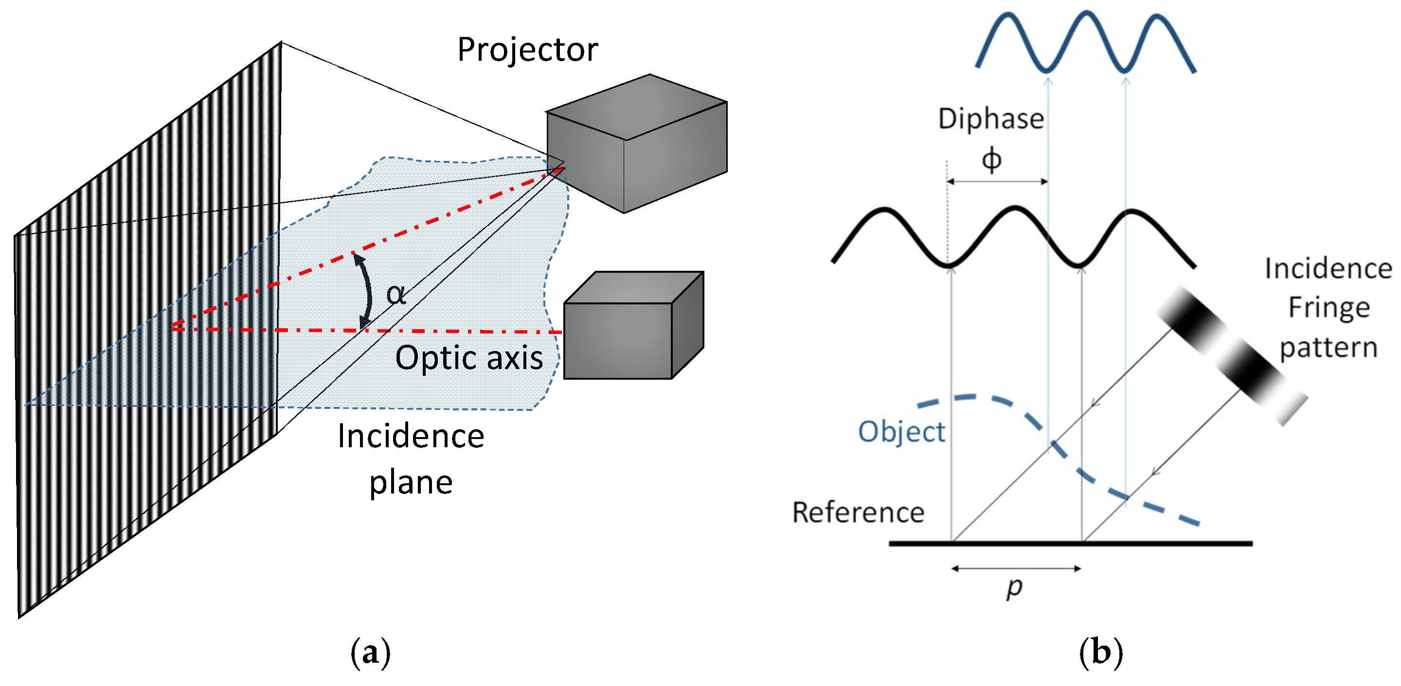
2.1. Fringe Projection
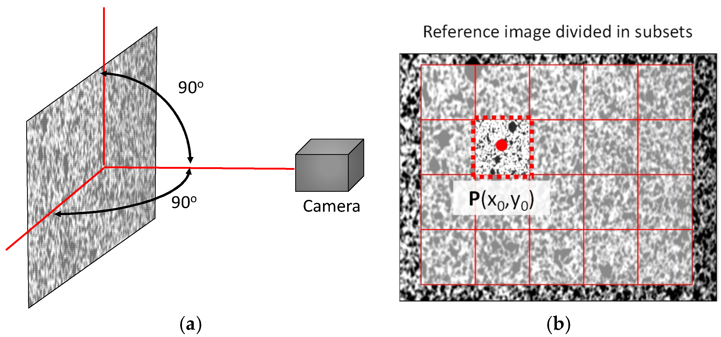
2.2. Digital Image Correlation
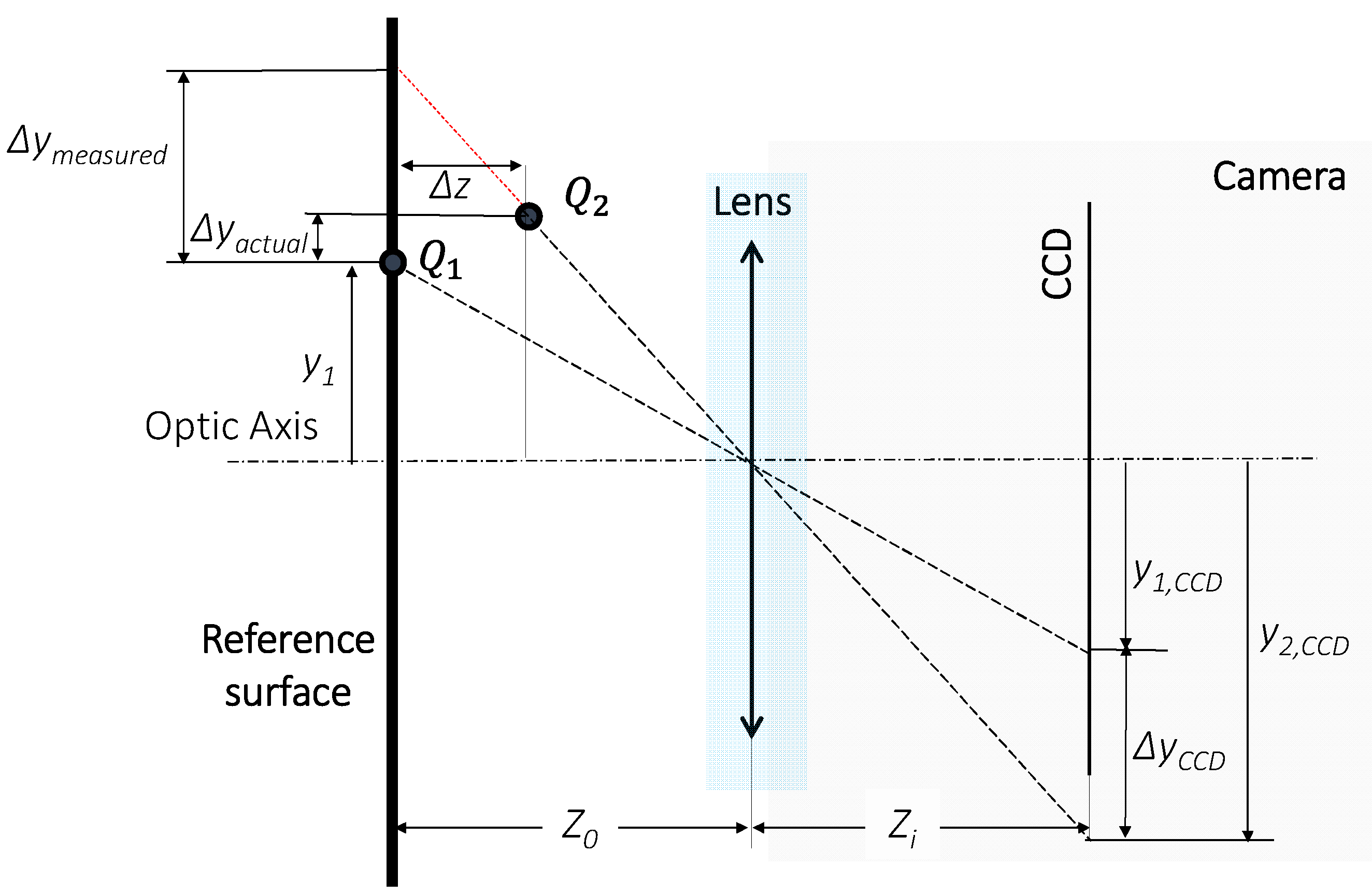
2.3. In-Plane Displacement Correction
3. Experimental Procedure
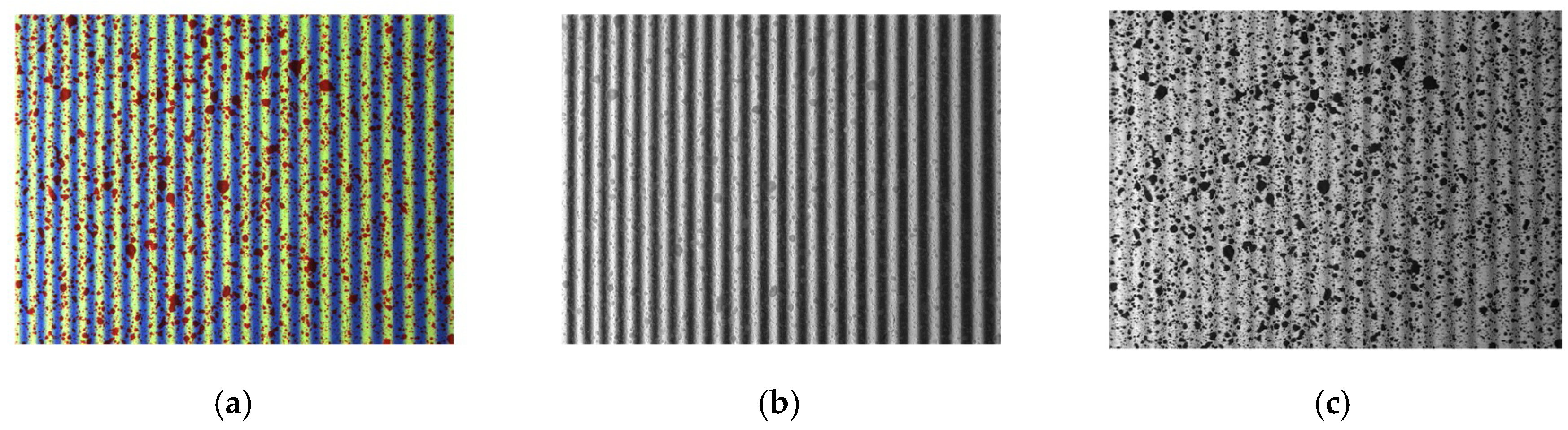
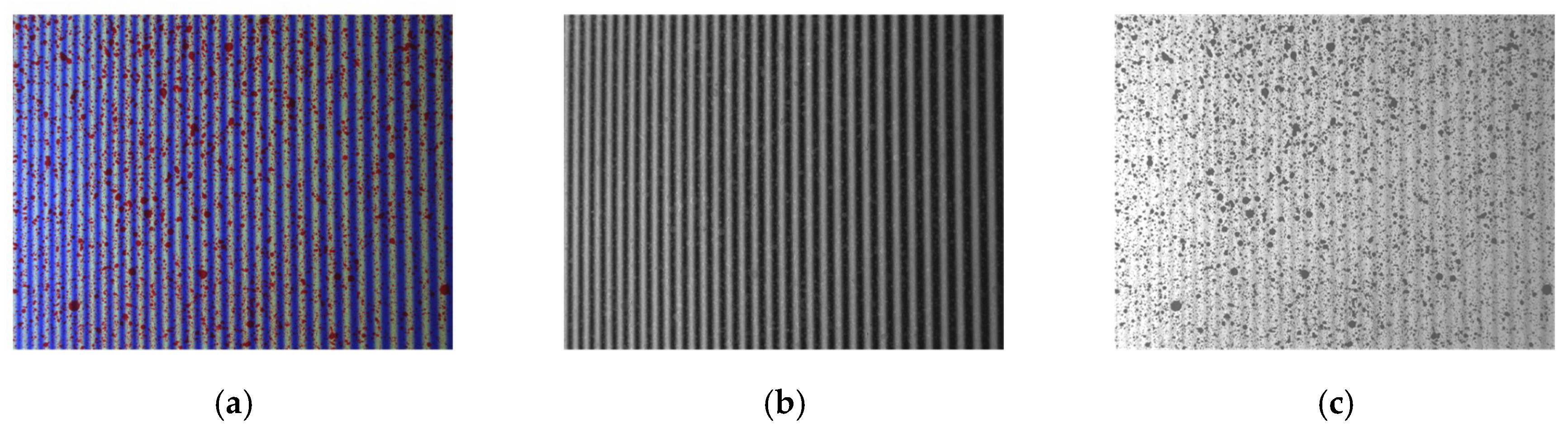
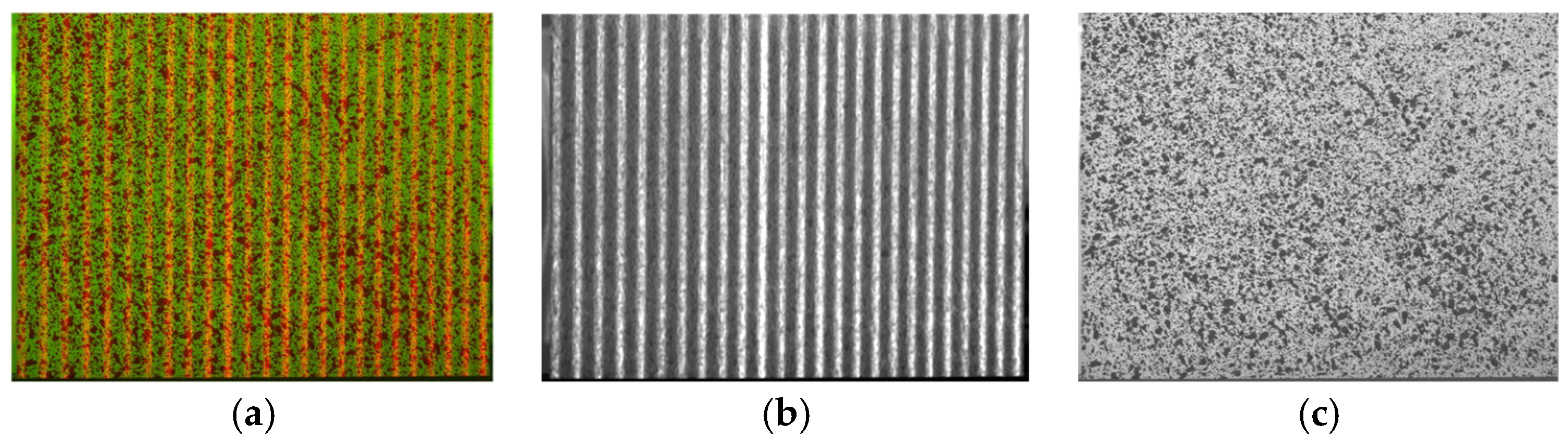
3.1. RGB Colour Pattern Encoding
3.1.1. Three-Sensor Camera
3.1.2. Laser Projection
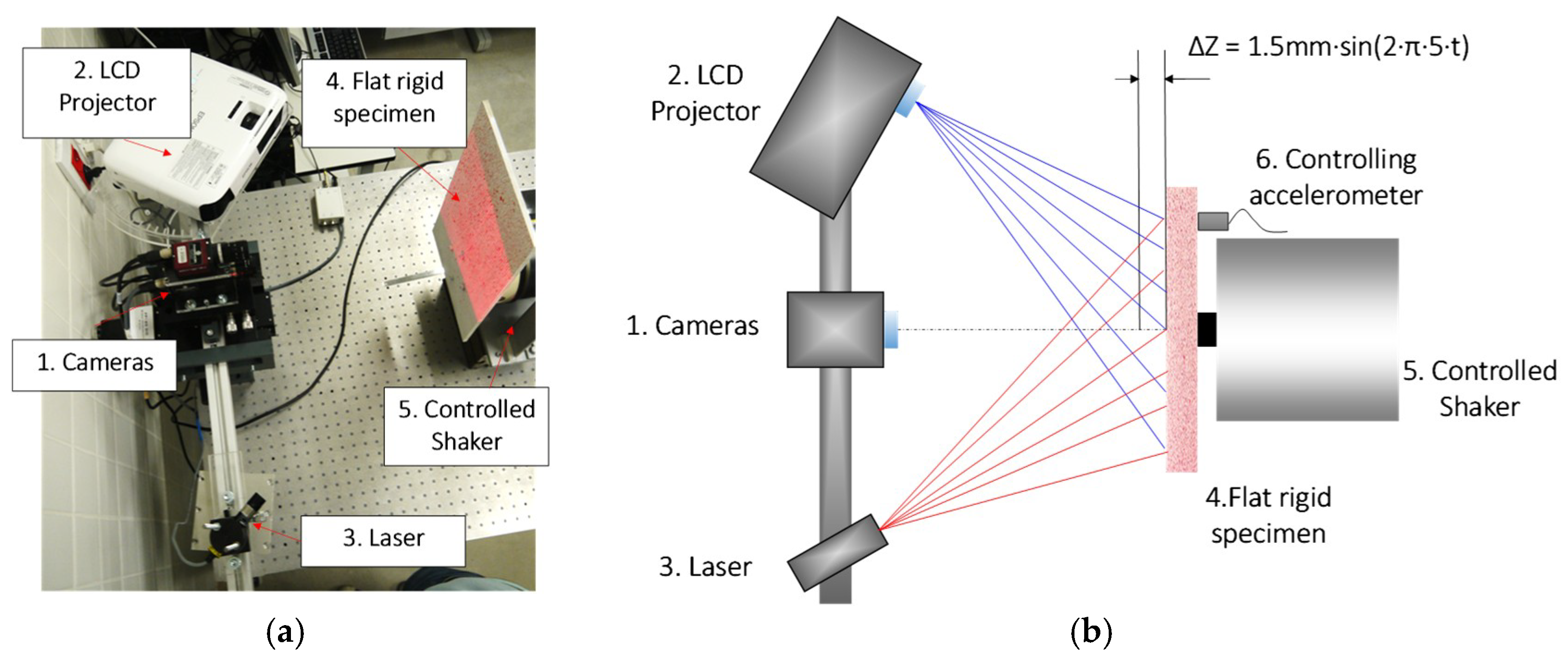
3.2. Experimental Set-Up
3.2.1. Vibration Test
3.2.2. Bending Test
4. Results
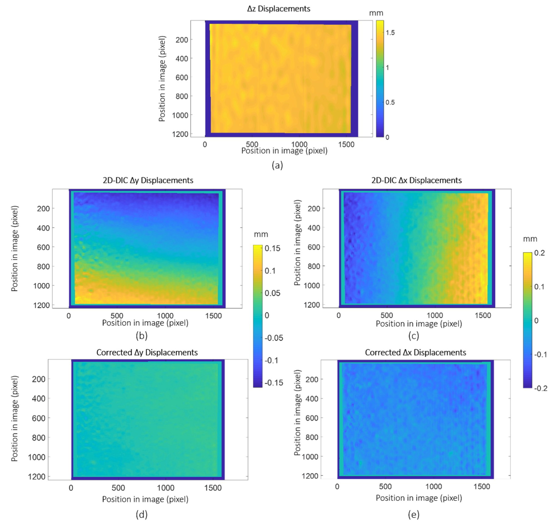
4.1. Vibration Test
4.2. Bending Test
5. Conclusions
Author Contributions
Funding
Conflicts of Interest
References
- Cloud, G. Optical methods in experimental mechanics. Exp. Tech. 2011, 35, 3–6. [Google Scholar] [CrossRef]
- Sharpe, W.N. Springer Handbook of Experimental Solid Mechanics; Springer: New York, NY, USA, 2008. [Google Scholar]
- Patterson, E.A.; Wang, Z.F. Simultaneous observation of phase-stepped images for automated photoelasticity. J. Strain Anal. Eng. Des. 2005, 33, 1–15. [Google Scholar] [CrossRef]
- Patterson, E.A.; Wang, Z.F. Towards full field automated photoelastic analysis of complex components. Strain 1991, 27, 49–53. [Google Scholar] [CrossRef]
- Ramesh, K. Digital Photoelasticity—Advanced Techniques and Applications; Springer: Berlin/Heidelberg, Germany, 2000; ISBN 9783642640995. [Google Scholar]
- Sjödahl, M. Electronic Speckle Photography: Increased Accuracy by Nonintegral Pixel Shifting. Appl. Opt. 1994, 33, 6667–6673. [Google Scholar] [CrossRef] [PubMed]
- Takeda, M.; Ina, H.; Kobayashi, S. Fourier-transform method of fringe-pattern analysis for computer-based topography and interferometry. J. Opt. Soc. Am. 1982, 72, 156–160. [Google Scholar] [CrossRef]
- Takeda, M.; Mutoh, K. Fourier transform profilometry for the automatic measurement of 3-D object shapes. Appl. Opt. 1983, 22, 3977–3982. [Google Scholar] [CrossRef] [PubMed]
- Srinivasan, V.; Liu, H.C.; Halioua, M. Automated phase-measuring profilometry: A phase mapping approach. Appl. Opt. 1985, 24, 185–188. [Google Scholar] [CrossRef] [PubMed]
- Gorthi, S.S.; Rastogi, P. Fringe projection techniques: Whither we are? Opt. Lasers Eng. 2010, 48, 133–140. [Google Scholar] [CrossRef] [Green Version]
- Heredia-Ortiz, M.; Patterson, E.A. On the Industrial Applications of Moire and Fringe Projection Techniques. Strain 2003, 39, 95–100. [Google Scholar] [CrossRef]
- Kühmstedt, P.; Munckelt, C.; Heinze, M.; Bräuer-Burchardt, C.; Notni, G.H.G.; Notni, G.H.G.; Huang, P.S. Digital Fringe Projection in 3D Shape Measurement—An Error Analysis. Opt. Eng. 2003, 5144, 66160B. [Google Scholar] [CrossRef]
- Notni, G.H.; Notni, G. Digital Fringe Projection in 3D Shape Measurement—An Error Analysis. In Proceedings of the SPIE 5144, Munich, Germany, 30 May 2003. [Google Scholar]
- Chen, L.C.; Huang, C.C. Miniaturized 3D surface profilometer using digital fringe projection. Meas. Sci. Technol. 2005, 16, 1061. [Google Scholar] [CrossRef]
- Huang, P.S. High-speed 3-D shape measurement based on digital fringe projection. Opt. Eng. 2003, 42, 163–169. [Google Scholar] [CrossRef]
- Sutton, M.A.; Orteu, J.J.; Schreier, H. Image Correlation for Shape, Motion and Deformation Measurements: Basic Concepts, Theory and Applications; Springer US: Boston, MA, USA, 2009; 322p, ISBN 978-0-387-78746-6. [Google Scholar]
- Molina-Viedma, A.J.; Felipe-Sesé, L.; López-Alba, E.; Díaz, F. High frequency mode shapes characterisation using Digital Image Correlation and phase-based motion magnification. Mech. Syst. Signal Process. 2018, 102, 245–261. [Google Scholar] [CrossRef]
- Molina-Viedma, Á.J.; López-Alba, E.; Felipe-Sesé, L.; Díaz, F.A. Full-field modal analysis during base motion excitation using high-speed 3D digital image correlation. Meas. Sci. Technol. 2017, 28, 105402. [Google Scholar] [CrossRef] [Green Version]
- Molina-Viedma, A.; López-Alba, E.; Felipe-Sesé, L.; Díaz, F.; Rodríguez-Ahlquist, J.; Iglesias-Vallejo, M. Modal Parameters Evaluation in a Full-Scale Aircraft Demonstrator under Different Environmental Conditions Using HS 3D-DIC. Materials 2018, 11, 230. [Google Scholar] [CrossRef] [PubMed]
- Molina-Viedma, A.J.; Felipe-Sesé, L.; López-Alba, E.; Díaz, F.A. 3D mode shapes characterisation using phase-based motion magnification in large structures using stereoscopic DIC. Mech. Syst. Signal Process. 2018, 108, 140–155. [Google Scholar] [CrossRef]
- Molina-Viedma, Á.; López-Alba, E.; Felipe-Sesé, L.; Díaz, F. Modal Identification in an Automotive Multi-Component System Using HS 3D-DIC. Materials 2018, 11, 241. [Google Scholar] [CrossRef] [PubMed]
- Felipe-Sesé, L.; López-Alba, E.; Hannemann, B.; Schmeer, S.; Diaz, F.A. A validation approach for quasistatic numerical/experimental indentation analysis in soft materials using 3D digital image correlation. Materials 2017, 10, 722. [Google Scholar] [CrossRef] [PubMed]
- Patterson, E.A.; Patki, A.S. On characterizing strain fields in impact-damaged composites using shape descriptors. Procedia IUTAM 2012, 4, 126–132. [Google Scholar] [CrossRef]
- Sebastian, C.; Hack, E.; Patterson, E. An approach to the validation of computational solid mechanics models for strain analysis. J. Strain Anal. Eng. Des. 2012, 48, 36–47. [Google Scholar] [CrossRef]
- Baronea, S.; Neria, P.; Paolia, A.; Razionale, A. Digital Image Correlation based on projected pattern for high frequency vibration measurements. Procedia Manuf. 2017, 11, 1592–1599. [Google Scholar] [CrossRef]
- Dekiff, M.; Berssenbrügge, P.; Kemper, B.; Denz, C.; Dirksen, D. Three-dimensional data acquisition by digital correlation of projected speckle patterns. Appl. Phys. B Lasers Opt. 2010, 99, 449–456. [Google Scholar] [CrossRef]
- Sutton, M.; Wolters, W.; Peters, W.; Ranson, W.; McNeill, S. Determination of displacements using an improved digital correlation method. Image Vis. Comput. 1983, 1, 133–139. [Google Scholar] [CrossRef]
- Sutton, M.A.; Chao, Y.J. Measurement of Strains in a Paper Tensile Specimen Using Computer Vision and Digital Image Correlation. Tappi J. 1988, 71, 173–175. [Google Scholar]
- Pan, B.; Wang, Z.; Lu, Z. Genuine full-field deformation measurement of an object with complex shape using reliability-guided digital image correlation. Opt. Express 2010, 18, 1011–1023. [Google Scholar] [CrossRef] [PubMed]
- Pan, B. Full-field strain measurement using a two-dimensional Savitzky-Golay digital differentiator in digital image correlation. Opt. Eng. 2007, 46, 033601. [Google Scholar] [CrossRef]
- Mares, C.; Barrientos, B.; Blanco, A. Measurement of transient deformation by color encoding. Opt. Express 2011, 19, 25712–25722. [Google Scholar] [CrossRef] [PubMed]
- Barrientos, B.; Cerca, M.; García-Márquez, J.; Hernández-Bernal, C. Three-dimensional displacement fields measured in a deforming granular-media surface by combined fringe projection and speckle photography. J. Opt. A Pure Appl. Opt. 2008, 10, 104027. [Google Scholar] [CrossRef]
- Tay, C.J.; Quan, C.; Wu, T.; Huang, Y.H. Integrated method for 3-D rigid-body displacement measurement using fringe projection. Opt. Eng. 2004, 43, 1152–1160. [Google Scholar] [CrossRef]
- Shi, H.; Ji, H.; Yang, G.; He, X. Shape and deformation measurement system by combining fringe projection and digital image correlation. Opt. Lasers Eng. 2013, 51, 47–53. [Google Scholar] [CrossRef]
- Tay, C.J.; Quan, C.; Huang, Y.H.; Fu, Y. Digital image correlation for whole field out-of-plane displacement measurement using a single camera. Opt. Commun. 2005, 251, 23–36. [Google Scholar] [CrossRef]
- Quan, C.; Tay, C.J.; Huang, Y.H. 3-D deformation measurement using fringe projection and digital image correlation. Opt. Int. J. Light Electron Opt. 2004, 115, 164–168. [Google Scholar] [CrossRef]
- Siegmann, P.; Álvarez-Fernández, V.; Díaz-Garrido, F.; Patterson, E.A. A simultaneous in- and out-of-plane displacement measurement method. Opt. Lett. 2011, 36, 10–12. [Google Scholar] [CrossRef] [PubMed]
- Nguyen, T.N.; Huntley, J.M.; Burguete, R.L.; Coggrave, C.R. Multiple-view shape and deformation measurement by combining fringe projection and digital image correlation. Strain 2012, 48, 256–266. [Google Scholar] [CrossRef]
- Felipe-Sesé, L.; Siegmann, P.; Díaz, F.A.; Patterson, E.A. Simultaneous in-and-out-of-plane displacement measurements using fringe projection and digital image correlation. Opt. Lasers Eng. 2014, 52, 66–74. [Google Scholar] [CrossRef]
- Felipe-Sesé, L.; Siegmann, P.; Díaz, F.A.; Patterson, E.A. Integrating fringe projection and digital image correlation for high-quality measurements of shape changes. Opt. Eng. 2014, 53, 044106. [Google Scholar] [CrossRef]
- Ramanath, R.; Snyder, W.E.; Bilbro, G.L.; Sander, W.A. Demosaicking methods for Bayer color arrays. J. Electron. Imaging 2002, 11, 306–316. [Google Scholar] [CrossRef]
- Pan, B.; Qian, K.; Xie, H.; Asundi, A. Two-dimensional digital image correlation for in-plane displacement and strain measurement: A review. Meas. Sci. Technol. 2009, 20, 1–17. [Google Scholar] [CrossRef]
- Felipe-Sesé, L.; Díaz, F.A. Damage methodology approach on a composite panel based on a combination of Fringe Projection and 2D Digital Image Correlation. Mech. Syst. Signal Process. 2018, 101, 467–479. [Google Scholar] [CrossRef]
- Felipe-Sesé, L.; Díaz, F.A.; Patterson, E.A. Exploiting measurement-based validation for a high-fidelity model of dynamic indentation of a hyperelastic material. Int. J. Solids Struct. 2016, 97, 520–529. [Google Scholar] [CrossRef]
- Mares, C.; Barrientos, B.; Valdivia, R. Three-dimensional displacement in multi-colored objects. Opt. Express 2017, 25, 11652–11672. [Google Scholar] [CrossRef] [PubMed]
- Sutton, M.A.; Yan, J.H.; Tiwari, V.; Schreier, H.W.; Orteu, J.J. The effect of out-of-plane motion on 2D and 3D digital image correlation measurements. Opt. Lasers Eng. 2008, 46, 746–757. [Google Scholar] [CrossRef] [Green Version]
- Siegmann, P.; Felipe-Sese, L.; Diaz-Garrido, F. Improved 3D displacement measurements method and calibration of a combined fringe projection and 2D-DIC system. Opt. Lasers Eng. 2017, 88, 255–264. [Google Scholar] [CrossRef]


| LCD Projection | Laser Projection | ||||
|---|---|---|---|---|---|
| Displacement | Mean Error (mm) | Standard Deviation (mm) | Displacement | Mean Error (mm) | Standard Deviation (mm) |
| Δx | 0.0268 | 0.0112 (0.083 px) | Δx | 0.0148 | 0.0055 (0.041 px) |
| Δy | 0.0218 | 0.0164 (0.1214 px) | Δy | 0.0084 | 0.0064 (0.047 px) |
| Δz | 0.07 | 0.0071 (0.058 rad) | Δz | 0.11 | 0.0084 (0.067 rad) |
© 2018 by the authors. Licensee MDPI, Basel, Switzerland. This article is an open access article distributed under the terms and conditions of the Creative Commons Attribution (CC BY) license (http://creativecommons.org/licenses/by/4.0/).
Share and Cite
Felipe-Sesé, L.; Molina-Viedma, Á.J.; López-Alba, E.; Díaz, F.A. RGB Colour Encoding Improvement for Three-Dimensional Shapes and Displacement Measurement Using the Integration of Fringe Projection and Digital Image Correlation. Sensors 2018, 18, 3130. https://doi.org/10.3390/s18093130
Felipe-Sesé L, Molina-Viedma ÁJ, López-Alba E, Díaz FA. RGB Colour Encoding Improvement for Three-Dimensional Shapes and Displacement Measurement Using the Integration of Fringe Projection and Digital Image Correlation. Sensors. 2018; 18(9):3130. https://doi.org/10.3390/s18093130
Chicago/Turabian StyleFelipe-Sesé, Luis, Ángel Jesús Molina-Viedma, Elías López-Alba, and Francisco A. Díaz. 2018. "RGB Colour Encoding Improvement for Three-Dimensional Shapes and Displacement Measurement Using the Integration of Fringe Projection and Digital Image Correlation" Sensors 18, no. 9: 3130. https://doi.org/10.3390/s18093130