
End-to-End Simulation for a Forest-Dedicated Full-Waveform Lidar Onboard a Satellite Initialized from Airborne Ultraviolet Lidar Experiments

Abstract
:
1. Introduction
2. Methodology
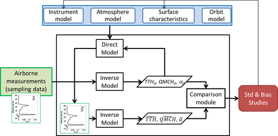
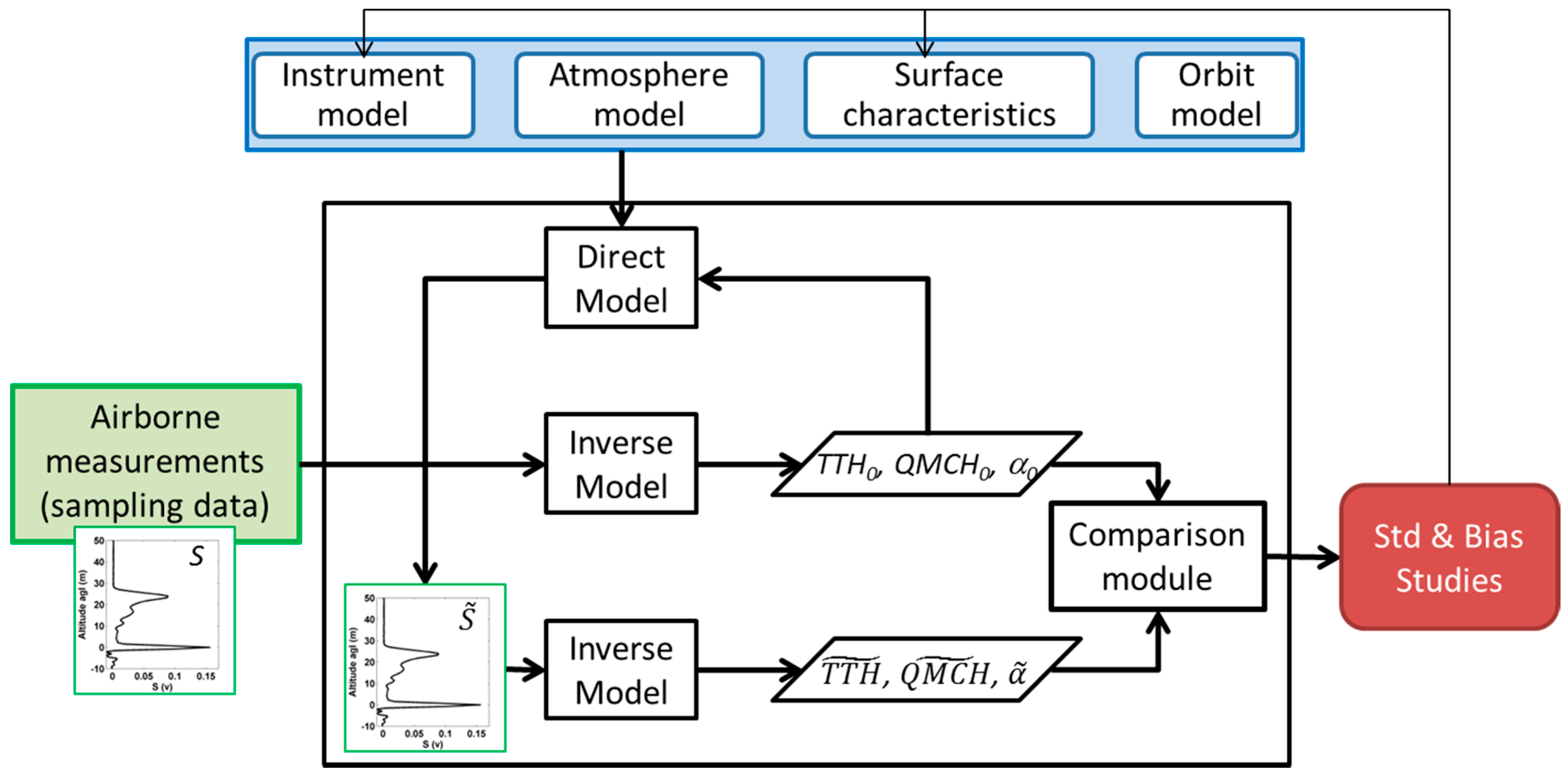
2.1. Overview


2.2. Direct Model
2.2.1. Instrument Model
2.2.2. Atmospheric Model

| Wavelength | λ (nm) | 355 | 1064 | |
|---|---|---|---|---|
| Instrument model | QE | 85% | 35% | |
| G (A·W−1) | ~106 | ~103 | ||
| OE | 60% | 65% | ||
| Telescope diameter ø (receptor surface A) | 100 cm (~0.8 m2) | |||
| Δz (m) | 0.75 | |||
| Rc (Ω) | 50 | |||
| Atmosphere model | Ideal | AOT0 | 0.15 | 0.15 |
| MOT0 | 0.58 | 0.0065 | ||
| COT0 | 0 | 0 | ||
| Realistic | AOT | Varied 1 | ||
| COT | ||||
| Surface characteristics | ρg (sr−1) | 0.022 | ||
| BERsimu (sr−1) | 0.0065 | 0.0455 | ||
| BERadjusted (sr−1) | 0.005 | 0.035 | ||
| η | 1 | 0.96 | ||
2.2.3. Surface Characteristics
| Period | Pπ in “Mixed Forest” | Pπ in “Evergreen Needle Leaf” | Absorption Coefficient (1 − ω0) | |||
|---|---|---|---|---|---|---|
| 490 nm | 865 nm | 490 nm | 865 nm | 355 nm | 1064 nm | |
| January | 1.79 ± 0.32 | 1.52 ± 0.15 | 1.62 ± 0.48 | 1.57 ± 0.15 | ~0.95 | ~0.35 |
| July | 1.36 ± 0.42 | 1.36 ± 0.16 | 1.65 ± 0.44 | 1.53 ± 0.21 | ||
2.2.4. Platform Model
| Mission Lidar | Our Study | CALIPSO 1 | ICESat 1 | MERLIN 1 | ADM-Aeolus 1 | ISS |
|---|---|---|---|---|---|---|
| ULICE | CALIOP | GLAS | IPDA | ALADIN | - | |
| Orbit altitude zp (km) | 0.35 | 705 | 600 | 506 | 400 | 350 |
| Wavelength λ (nm) | 355 | 1064 | 1064 | 1645 | 355 | - |
| Laser Pulse Energy E (mJ) | 0.007 2 | 110 | 73 | 9 | 120 | - |
| QE | 20% | 33% | 35% | 60% | 85% | - |
| OE | 26% | 64% | 55% | 65% | 60% | - |
| Telescope diameter (cm) (surface A (m2)) | 15 (0.02) | 100 (0.79) | 100 (0.79) | 55 (0.24) | 150 (1.77) | - |
| Δz (m) | 0.75 | * | 0.15 | * | * | - |
2.3. Inverse Model
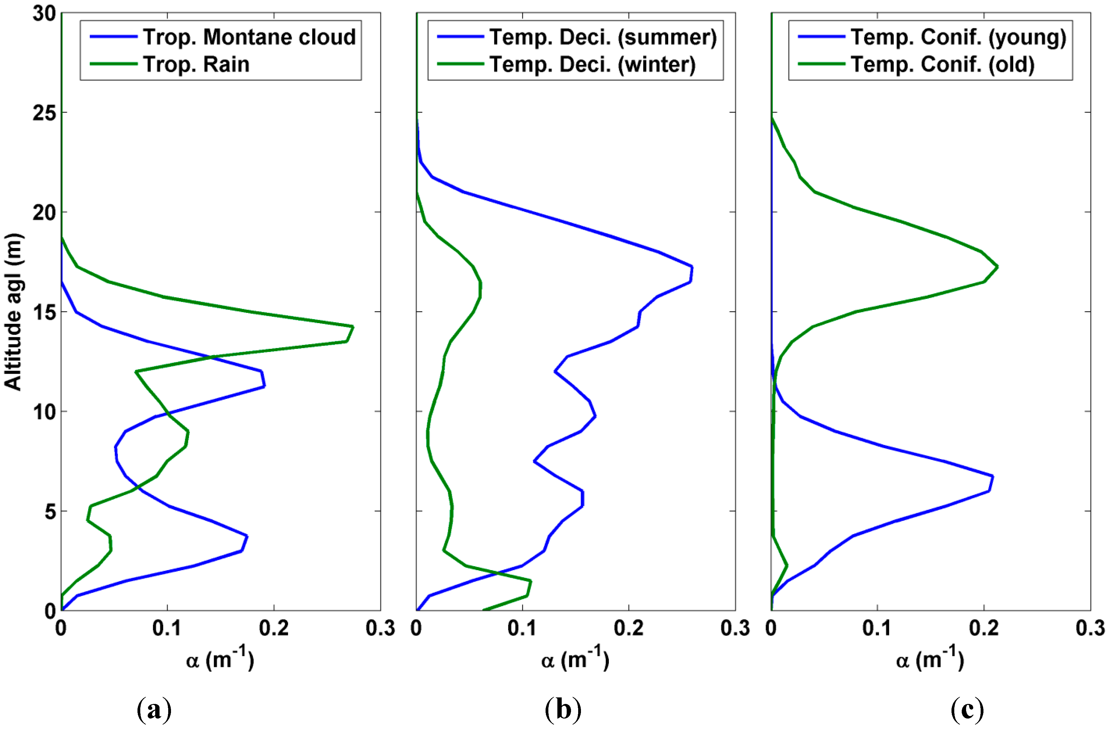
2.4. Sampling Sites
| Forest Sites | Land Cover1 | Main Tree Species | Location | Sampling Date | Sampling Area | Laser Shots |
|---|---|---|---|---|---|---|
| Landes | Temp.Conif. | Maritime pins | 44°9ʹN, 1°9ʹW | September 2008 | 170 ha | 62.3 × 10³ |
| Fontainebleau | Temp.Deci. Temp.Conif. | Oaks, Sylvester pines, Hornbeams and Beeches | 48°24ʹN, 2°38ʹE | November 2010 | 25 ha | 86.9 × 10³ |
| June 2012 | 4000 ha | 1.2 × 10⁶ | ||||
| March 2013 | 5 ha | 41.8 × 10³ | ||||
| OHP2 Region | Temp.Deci. Plantation | White oaks Poplars | 43°49ʹN, 5°49ʹE | May 2012 | 10 ha | 29.5 × 10³ |
| Réunion Island | Trop.Rain | Labourdonnaisia calophylloides | 21°4ʹS, 55°30ʹE | May 2014 | 5 ha | 12 × 103 |
| Trop.montane cloud | Acacia heterophylla | 21°21ʹS, 55°44ʹE | May 2014 | 420 ha | 48.4 ×10³ |


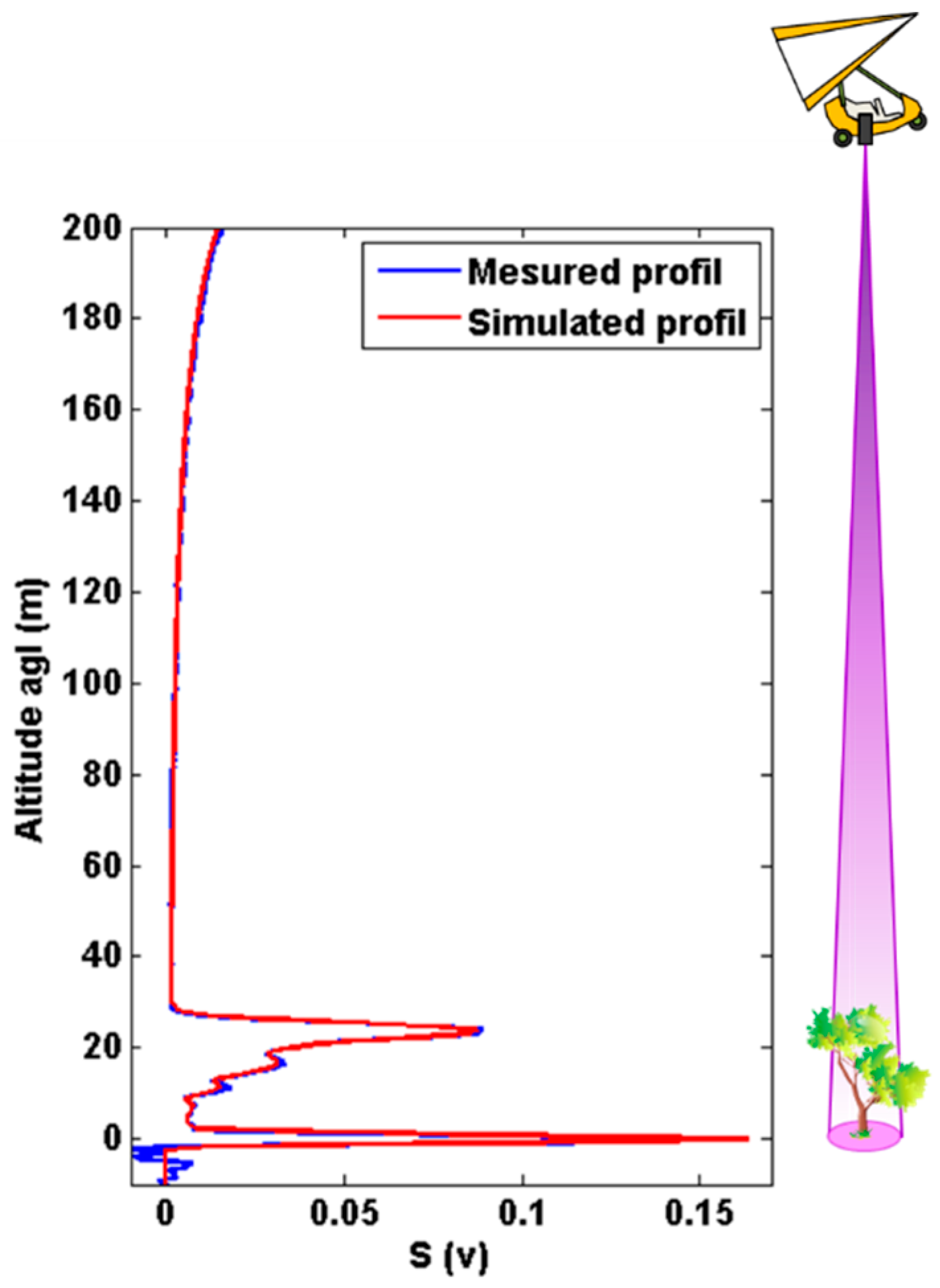
2.5. Adjustment of Parameters: Relevance of the Direct Model

3. End-to-End Modeling
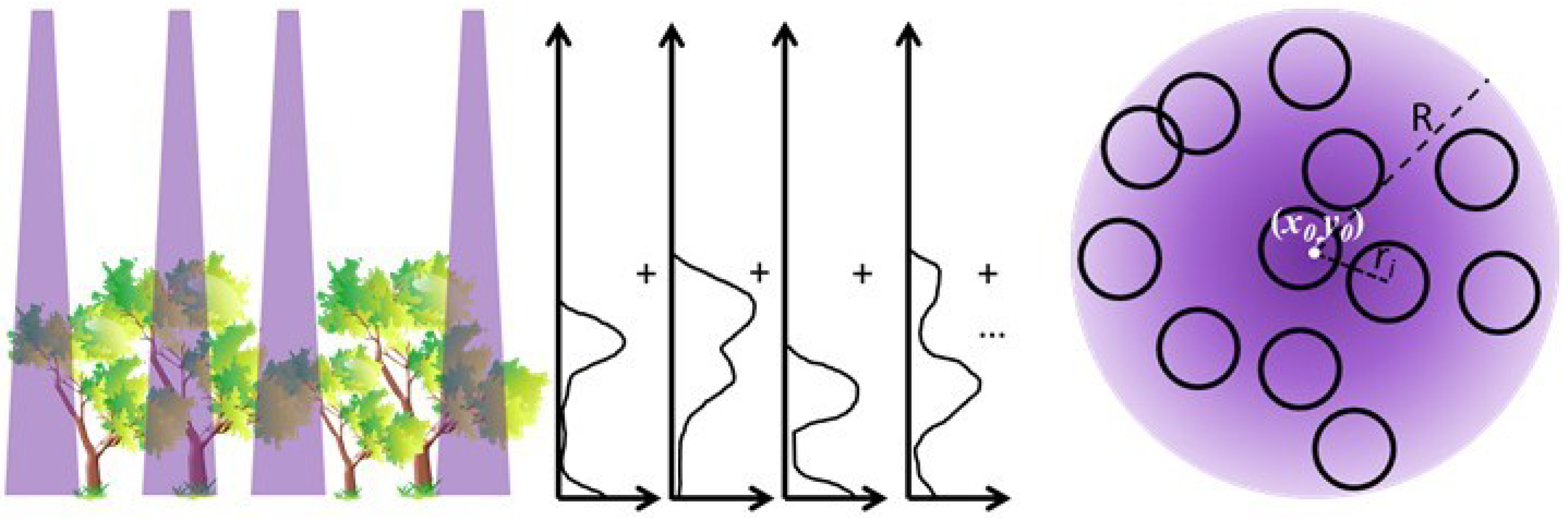
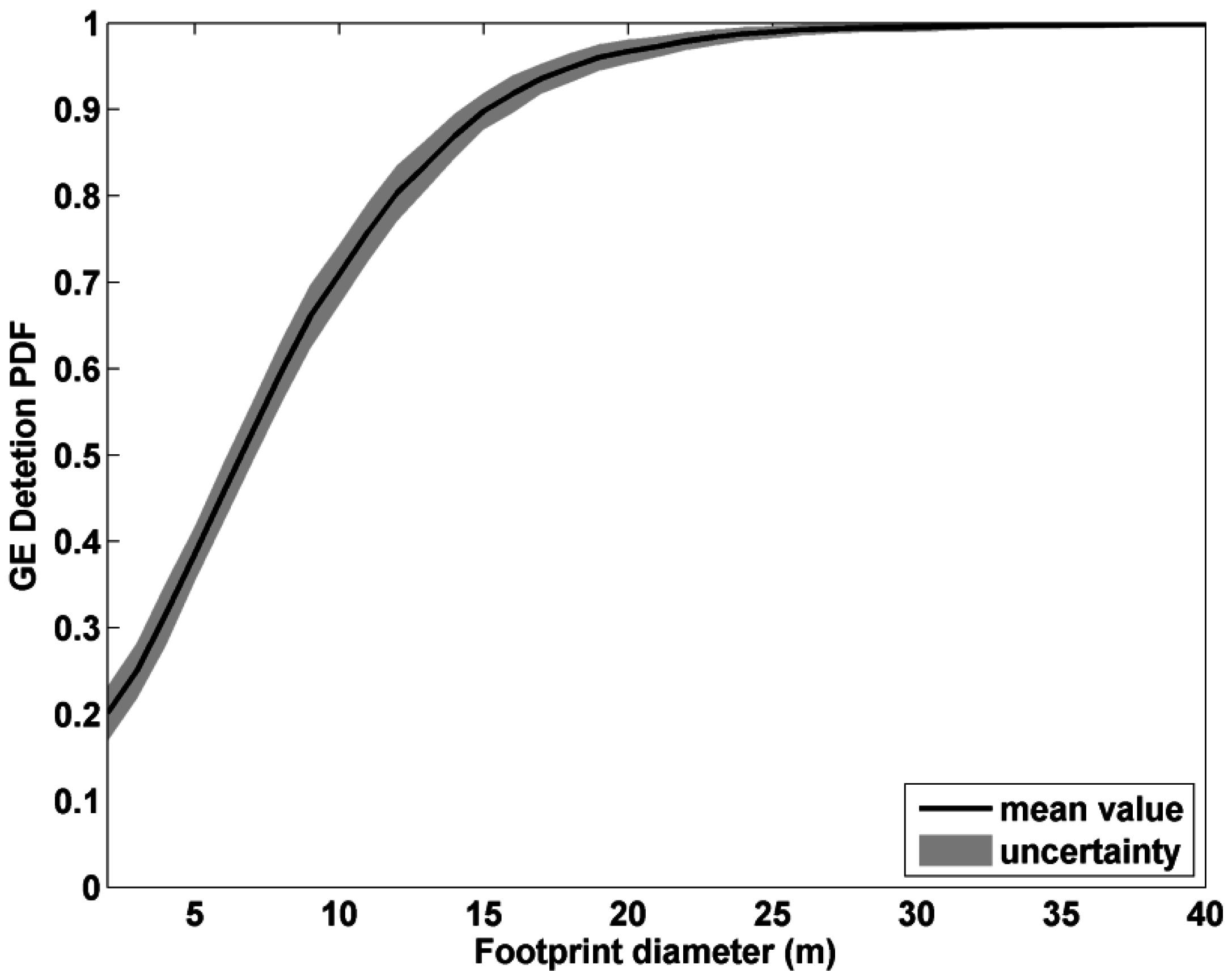
3.1. Laser Footprint Size


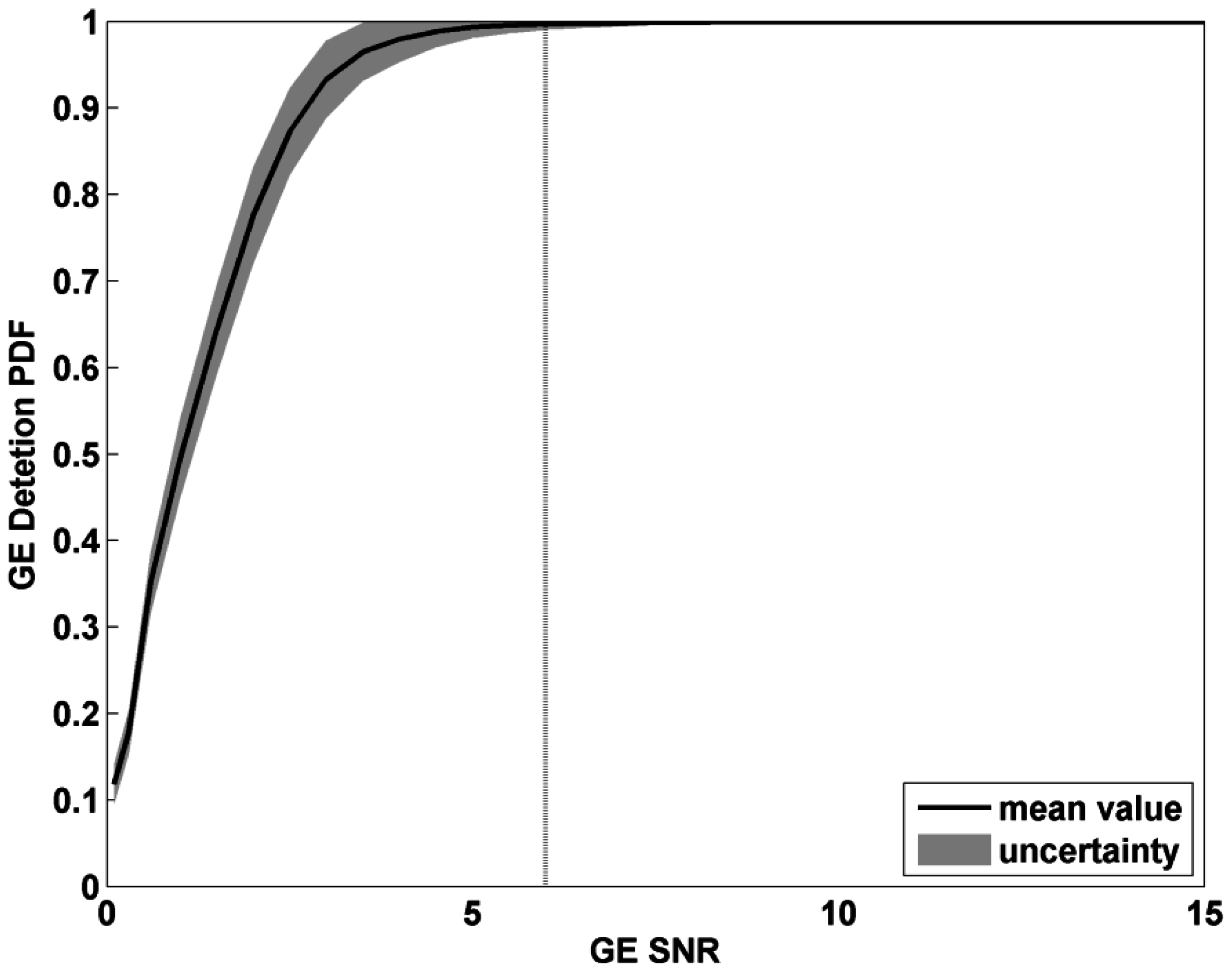
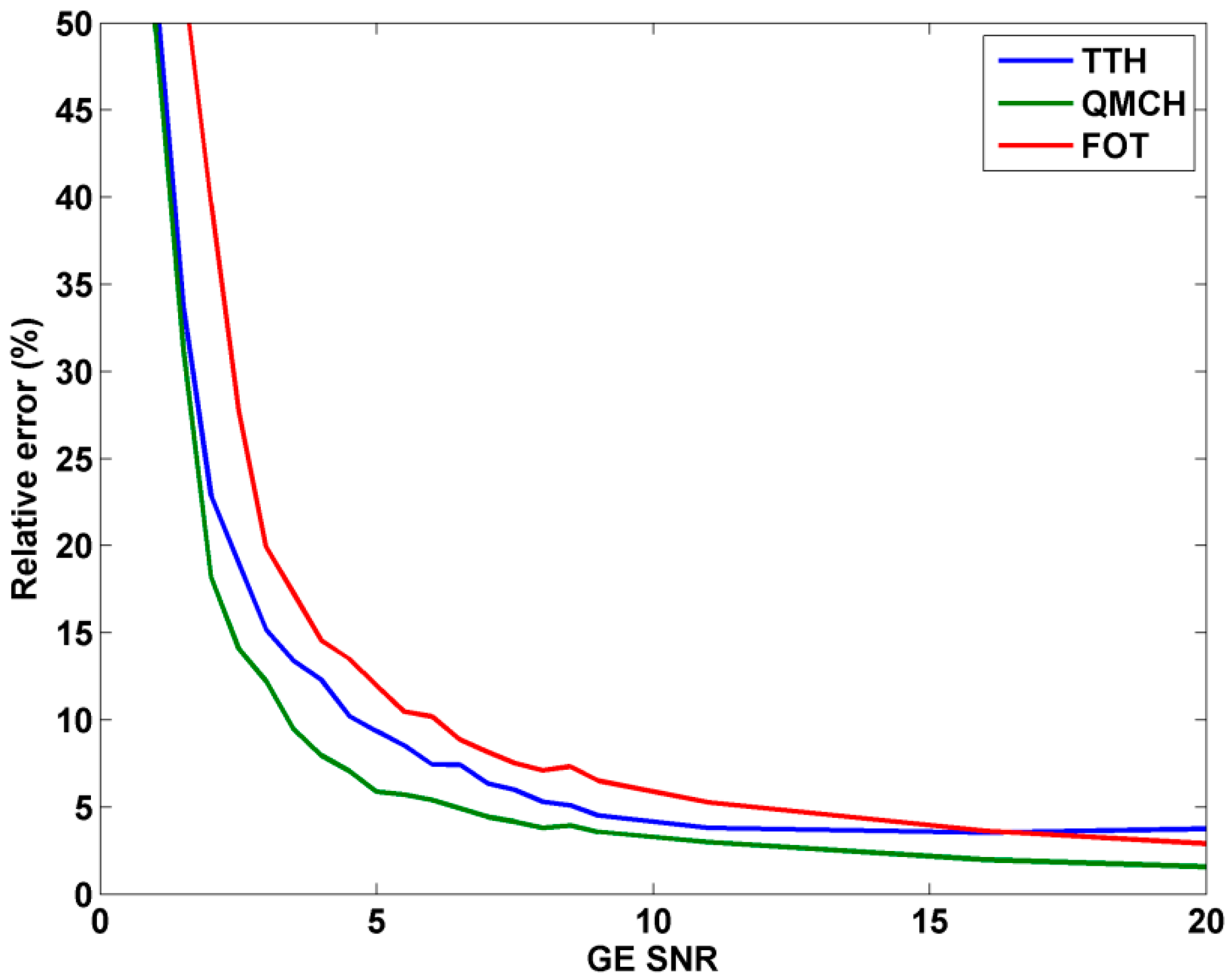
3.2. Optimal SNR and Related Uncertainties


3.3. Lidar Signal Distortion
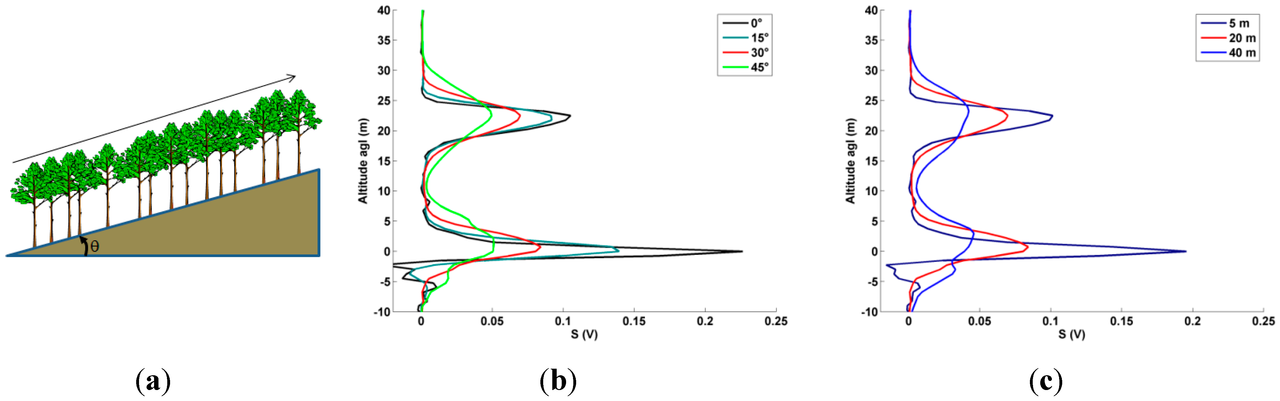
3.3.1. Surface Slope

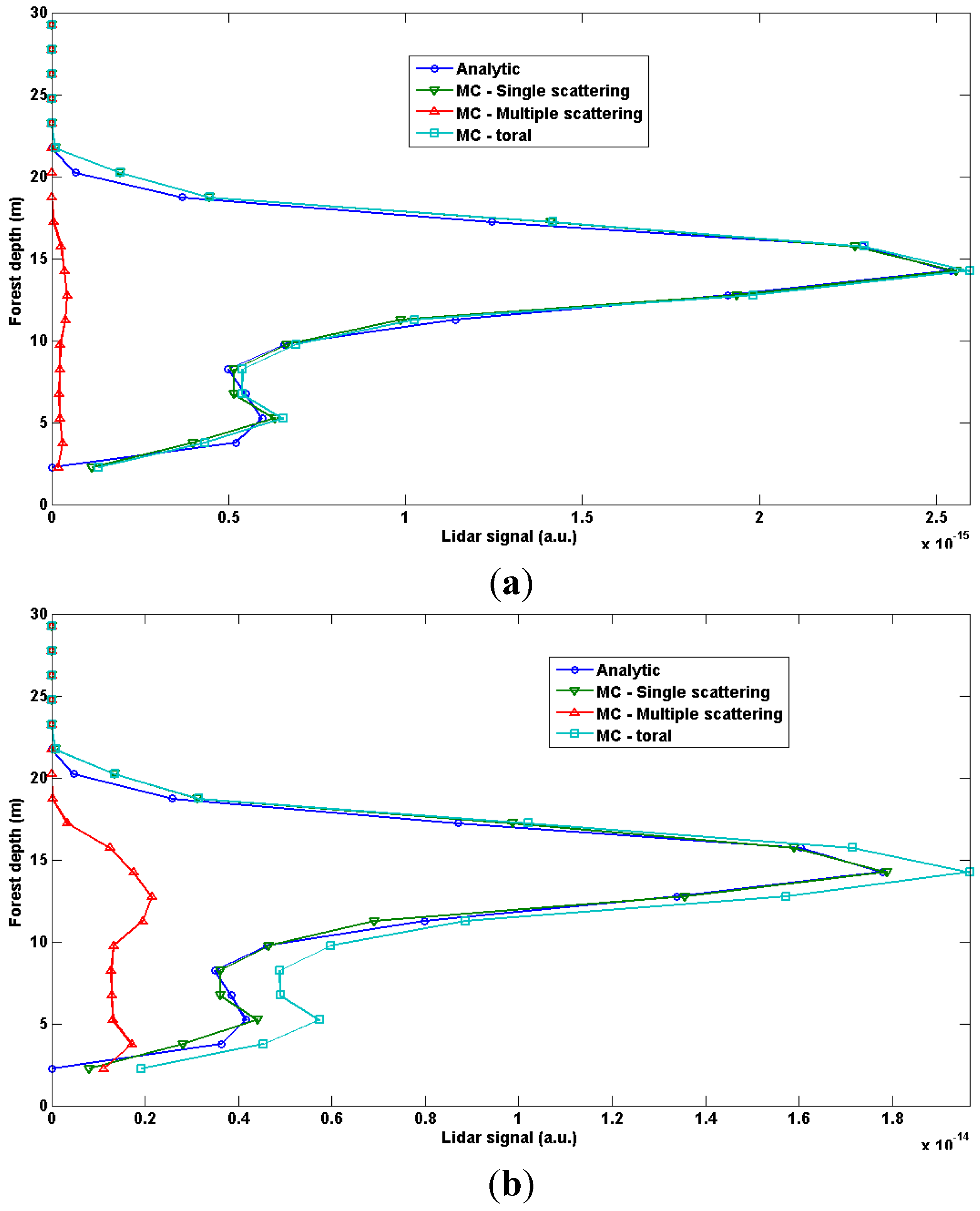
3.3.2. Multiple Scattering Effects

4. Link Budget
4.1. Link Budget under Ideal Atmospheric Conditions
| Mission | CALIPSO | ICESat | MERLIN | ADM-Aeolus | |
| Lidar | CALIOP | GLAS | IPDA | ALADIN | |
| Orbit altitude zp (km) | 705 | 600 | 506 | 400 | |
| GE SNR | FOT = 1 | 24.5 | 10.0 | 9.1 | 12.9 |
| FOT = 2 | 14.8 | 6.1 | 5.5 | 7.9 | |
| Orbit | CALIPSO | ICESat | MERLIN | ADM-Aeolus | ISS | ||
|---|---|---|---|---|---|---|---|
| Orbit altitude zp (km) | 705 | 600 | 506 | 400 | 350 | ||
| Required laser pulse energy | Forest class | Forest area proportion | |||||
| E (mJ) at 355 nm | FOT ≤ 1 | 30% | 333.6 | 241.7 | 171.9 | 107.4 | 82.2 |
| FOT ≤ 2 | 75% | 906.9 | 656.9 | 467.2 | 292 | 223.5 | |
| E (mJ) at 1064 nm | FOT ≤ 1 | 30% | 11.4 | 8.3 | 5.9 | 3.7 | 2.8 |
| FOT ≤ 2 | 75% | 31.0 | 22.5 | 16.0 | 10.0 | 7.7 | |
| FOT ≤ 3 | 92% | 84.4 | 61.1 | 43.5 | 27.2 | 20.8 | |
| FOT ≤ 4 | 98% | 229.4 | 166.1 | 118.2 | 73.8 | 56.5 | |
| Example: laser pulse energy E = 100 mJ at the wavelength of 1064 nm | |||||||
| TOTmax for good detection (TOT = FOT/2 + τ, Equation (4)) | 1.74 | 1.90 | 2.07 | 2.31 | 2.44 | ||
4.2. Link Budget under Realistic Atmospheric Conditions
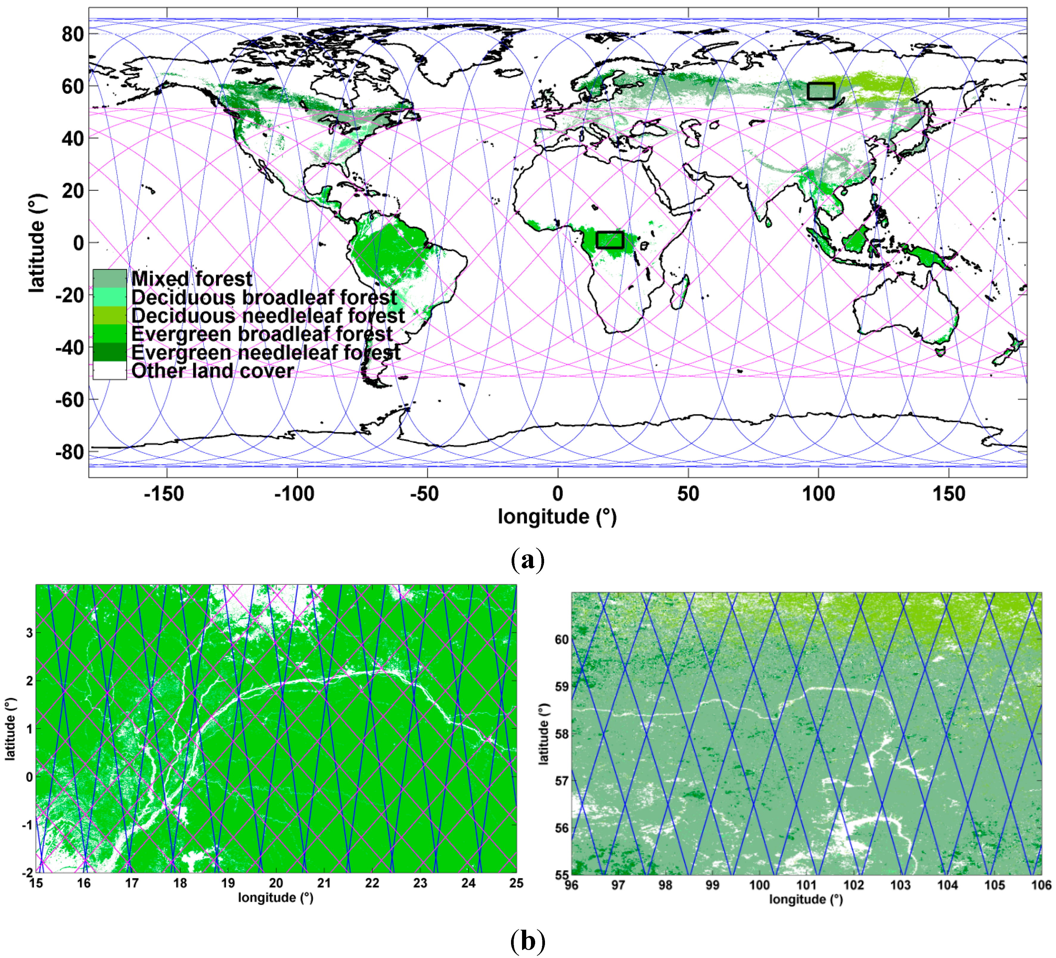
4.2.1. Study Areas

4.2.2. Study Periods
4.2.3. Orbit Simulation
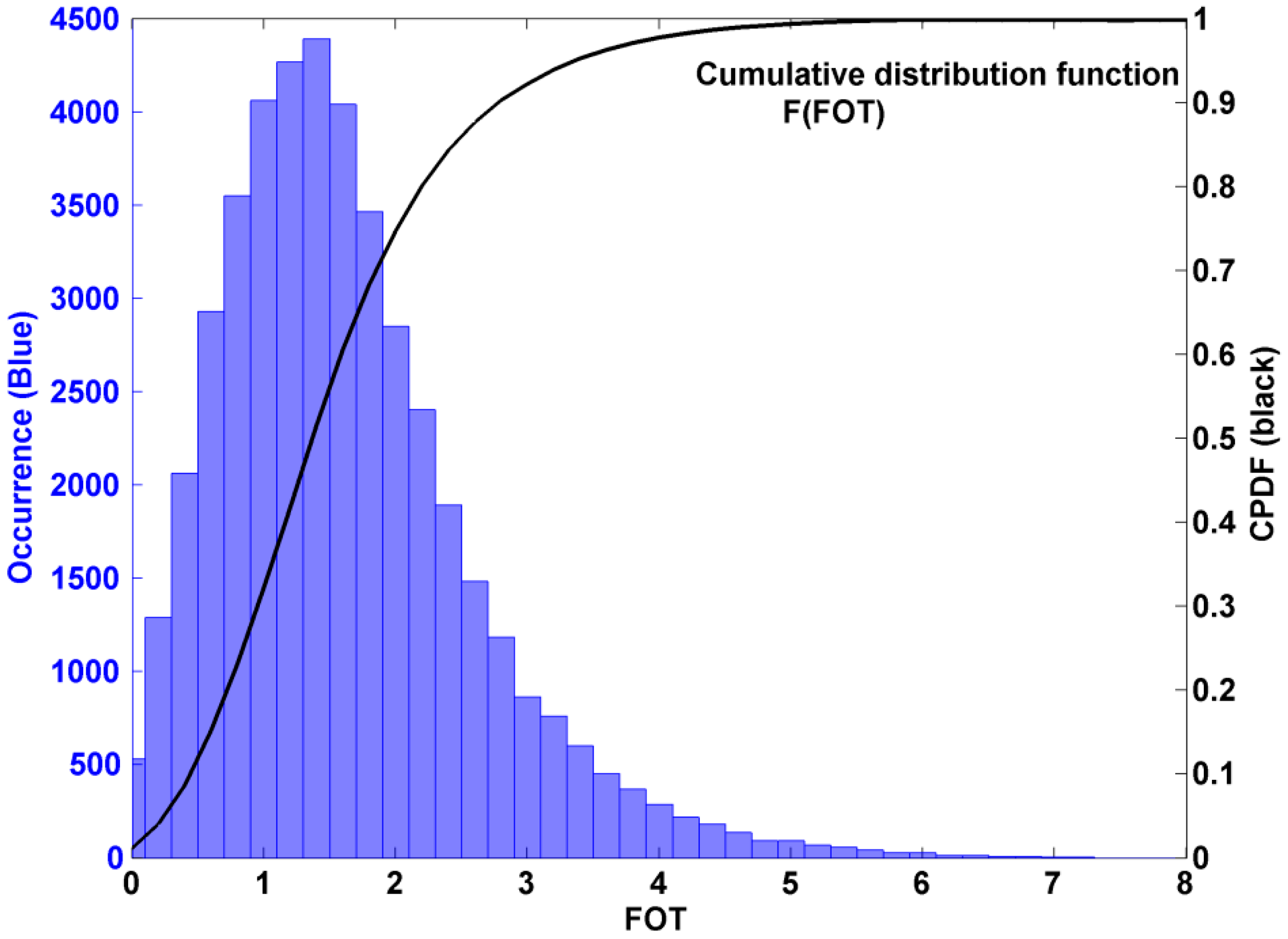
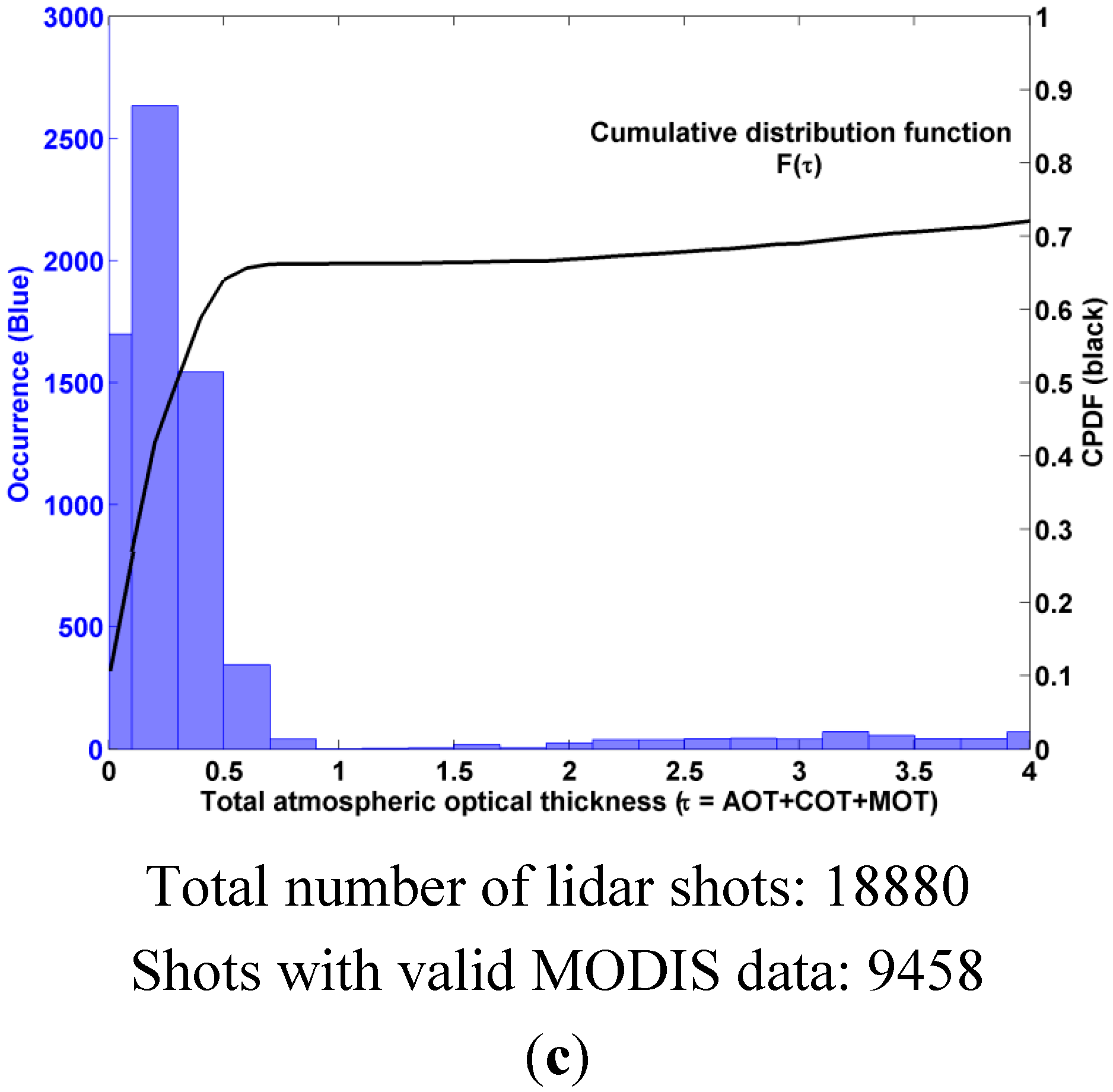
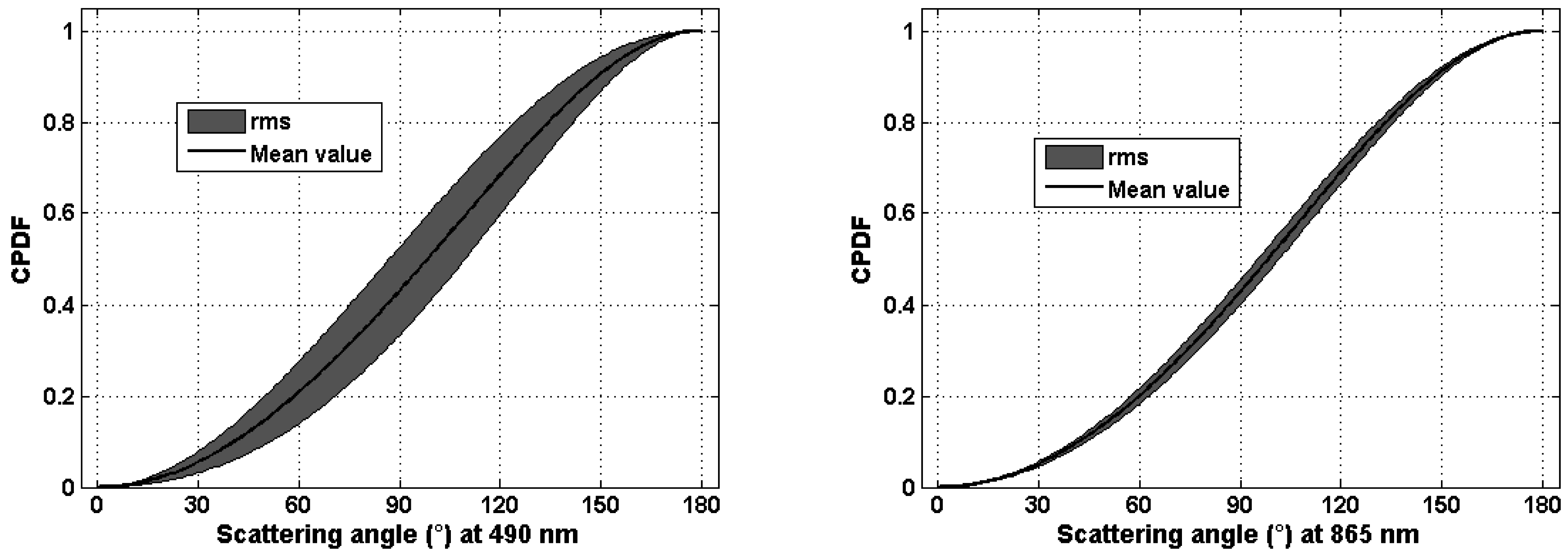
4.2.4. Atmospheric Distributions


4.2.5. Discussion on Probability of Good Detections for One Satellite Pass
4.2.6. Number of Satellite Revisits
5. Discussion and Conclusions
Acknowledgment
Author Contributions
Appendix A: Sources of Noise
Appendix B: Bidirectional Reflectance Distribution Function (BRDF) Retrieval

Conflicts of Interest
References
- Ciccioli, P.; Brancaleoni, E.; Frattoni, M.; di Palo, V.; Valentini, R.; Tirone, G.; Seufert, G.; Bertin, N.; Hansen, U.; Csiky, O.; et al. Emission of reactive terpene compounds from orange orchards and their removal by within-canopy processes. J. Geophys. Res. 1999, 104, 8077–8094. [Google Scholar] [CrossRef]
- Makar, P.A.; Fuentes, J.D.; Wang, D.; Staebler, R.M.; Wiebe, H.A. Chemical processing of biogenic hydrocarbons within and above a temperate deciduous forest. J. Geophys. Res. 1999, 104, 3581–3603. [Google Scholar] [CrossRef]
- Fuentes, J.D.; Gu, L.; Lerdau, M.; Atkinson, R.; Baldocchi, D.; Bottenheim, J.W.; Ciccioli, P.; Lamb, B.; Geron, C.; Guenther, A.; et al. Biogenic Hydrocarbons in the Atmospheric Boundary Layer: A Review. Bull. Am. Meteorol. Soc. 2000, 81, 1537–1575. [Google Scholar] [CrossRef]
- Forkel, R.; Klemm, O.; Graus, M.; Rappenglück, B.; Stockwell, W.R.; Grabmer, W.; Held, A.; Hansel, A.; Steinbrecher, R. Trace gas exchange and gas phase chemistry in a Norway spruce forest: A study with a coupled 1-dimensional canopy atmospheric chemistry emission model. Atmos. Environ. 2006, 40, 28–42. [Google Scholar] [CrossRef]
- Fowler, D.; Pilegaard, K.; Sutton, M.A.; Ambus, P.; Raivonen, M.; Duyzer, J.; Simpson, D.; Fagerli, H.; Fuzzi, S.; Schjoerring, J.K.; et al. Atmospheric composition change: Ecosystems-Atmosphere interactions. Atmos. Environ. 2009, 43, 5193–5267. [Google Scholar] [CrossRef]
- Tao, Z. A summer simulation of biogenic contributions to ground-level ozone over the continental United States. J. Geophys. Res. 2003, 108, 4404. [Google Scholar] [CrossRef]
- Thunis, P.; Cuvelier, C. Impact of biogenic emissions on ozone formation in the Mediterranean area—A BEMA modelling study. Atmos. Environ. 2000, 34, 467–481. [Google Scholar] [CrossRef]
- Tsigaridis, K.; Kanakidou, M. Global modelling of secondary organic aerosol in the troposphere: A sensitivity analysis. Atmos. Chem. Phys. 2003, 3, 1849–1869. [Google Scholar] [CrossRef]
- IPCC Climate Change 2013: The Physical Science Basis. Available online: http://www.ipcc.ch/pdf/assessment-report/ar5/wg1/WG1AR5_Frontmatter_FINAL.pdf (accessed on 21 April 2015).
- MacArthur, R.H.; MacArthur, J.W. On bird species diversity. Ecology 1961, 42, 594–598. [Google Scholar] [CrossRef]
- Hansen, A.J.; Rotella, J.J.; Kraska, M.P.V.; Brown, D. Spatial patterns of primary productivity in the Greater Yellowstone Ecosystem. Landsc. Ecol. 2000, 15, 505–522. [Google Scholar] [CrossRef]
- Hollinger, D.Y. Canopy Organization and Foliage Photosynthetic Capacity in a Broad-Leaved Evergreen Montane Forest. Funct. Ecol. 1989, 3, 53–62. [Google Scholar] [CrossRef]
- Brown, M.J.; Parker, G.G. Canopy light transmittance in a chronosequence of mixed-species deciduous forests. Can. J. For. Res. 1994, 24, 1694–1703. [Google Scholar] [CrossRef]
- Lefsky, M.A.; Cohen, W.B.; Acker, S.A.; Parker, G.G.; Spies, T.A.; Harding, D. Lidar remote sensing of the canopy structure and biophysical properties of Douglas-fir western hemlock forests. Remote Sens. Environ. 1999, 70, 339–361. [Google Scholar] [CrossRef]
- Lefsky, M.A.; Harding, D.; Cohen, W.B.; Parker, G.; Shugart, H.H. Surface lidar remote sensing of basal area and biomass in deciduous forests of eastern Maryland, USA. Remote Sens. Environ. 1999, 67, 83–98. [Google Scholar] [CrossRef]
- Horn, H.S. The Adaptive Geometry of Trees; Princeton University Press: Princeton, NJ, USA, 1971; Volume 1971. [Google Scholar]
- Hyde, P.; Dubayah, R.; Walker, W.; Blair, J.B.; Hofton, M.; Hunsaker, C. Mapping forest structure for wildlife habitat analysis using multi-sensor (LiDAR, SAR/InSAR, ETM+, Quickbird) synergy. Remote Sens. Environ. 2006, 102, 63–73. [Google Scholar] [CrossRef]
- Toan, T.; Quegan, S.; Woodward, I.; Lomas, M.; Delbart, N.; Picard, G. Relating Radar Remote Sensing of Biomass to Modelling of Forest Carbon Budgets. Clim. Chang. 2004, 67, 379–402. [Google Scholar] [CrossRef]
- Balzter, H.; Rowland, C.S.; Saich, P. Forest canopy height and carbon estimation at Monks Wood National Nature Reserve, UK, using dual-wavelength SAR interferometry. Remote Sens. Environ. 2007, 108, 224–239. [Google Scholar] [CrossRef]
- Garestier, F.; Dubois-Fernandez, P.C.; Champion, I. Forest Height Inversion Using High-Resolution P-Band Pol-InSAR Data. IEEE Trans. Geosci. Remote Sens. 2008, 46, 3544–3559. [Google Scholar] [CrossRef]
- Hall, F.G.; Bergen, K.; Blair, J.B.; Dubayah, R.; Houghton, R.; Hurtt, G.; Kellndorfer, J.; Lefsky, M.; Ranson, J.; Saatchi, S.; et al. Characterizing 3D vegetation structure from space: Mission requirements. Remote Sens. Environ. 2011, 115, 2753–2775. [Google Scholar] [CrossRef]
- Ni-Meister, W.; Jupp, D.L.B.; Dubayah, R. Modeling lidar waveforms in heterogeneous and discrete canopies. IEEE Trans. Geosci. Remote Sens. 2001, 39, 1943–1958. [Google Scholar] [CrossRef]
- Gastellu-Etchegorry, J.-P.; Yin, T.; Lauret, N.; Cajgfinger, T.; Gregoire, T.; Grau, E.; Feret, J.-B.; Lopes, M.; Guilleux, J.; Dedieu, G.; et al. Discrete Anisotropic Radiative Transfer (DART 5) for Modeling Airborne and Satellite Spectroradiometer and LIDAR Acquisitions of Natural and Urban Landscapes. Remote Sens. 2015, 7, 1667–1701. [Google Scholar] [CrossRef] [Green Version]
- Montesano, P.M.; Rosette, J.; Sun, G.; North, P.; Nelson, R.F.; Dubayah, R.O.; Ranson, K.J.; Kharuk, V. The uncertainty of biomass estimates from modeled ICESat-2 returns across a boreal forest gradient. Remote Sens. Environ. 2015, 158, 95–109. [Google Scholar] [CrossRef]
- Cuesta, J.; Chazette, P.; Allouis, T.; Flamant, P.H.; Durrieu, S.; Sanak, J.; Genau, P.; Guyon, D.; Loustau, D.; Flamant, C. Observing the forest canopy with a new ultra-violet compact airborne lidar. Sensors 2010, 10, 7386–7403. [Google Scholar] [CrossRef] [PubMed]
- Boudreau, J.; Nelson, R.F.; Margolis, H.A.; Beaudoin, A.; Guindon, L.; Kimes, D.S. Regional aboveground forest biomass using airborne and spaceborne LiDAR in Québec. Remote Sens. Environ. 2008, 112, 3876–3890. [Google Scholar] [CrossRef]
- Dubayah, R.O.; Drake, J.B. Lidar remote sensing for forestry. J. For. 2000, 98, 44–46. [Google Scholar]
- Reutebuch, S.E.; Andersen, H.; Mcgaughey, R.J.; Forest, L. Light detection and ranging (LIDAR ): an emerging tool for multiple resource inventory. J. For. 2005, 286–292. [Google Scholar]
- Berthier, S.; Chazette, P.; Couvert, P.; Pelon, J.; Dulac, F.; Thieuleux, F.; Moulin, C.; Pain, T. Desert dust aerosol columnar properties over ocean and continental Africa from Lidar in-Space Technology Experiment (LITE) and Meteosat synergy. J. Geophys. Res. 2006, 111, D21202. [Google Scholar] [CrossRef]
- Winker, D.M.; Hunt, W.H.; McGill, M.J. Initial performance assessment of CALIOP. Geophys. Res. Lett. 2007, 34. [Google Scholar] [CrossRef]
- Chazette, P.; Raut, J.-C.; Dulac, F.; Berthier, S.; Kim, S.-W.; Royer, P.; Sanak, J.; Loaëc, S.; Grigaut-Desbrosses, H. Simultaneous observations of lower tropospheric continental aerosols with a ground-based, an airborne, and the spaceborne CALIOP lidar system. J. Geophys. Res. 2010, 115. [Google Scholar] [CrossRef] [Green Version]
- Schutz, B.E.; Zwally, H.J.; Shuman, C.A.; Hancock, D.; DiMarzio, J.P. Overview of the ICESat Mission. Geophys. Res. Lett. 2005, 32. [Google Scholar] [CrossRef]
- Murooka, J.; Kobayashi, T.; Imai, T.; Suzuki, K.; Sakaizawa, D.; Yamakawa, S.; Sato, R.; Sawada, H.; Asai, K. Overview of Japan’s spaceborne vegetation lidar mission. Proc. SPIE 2013, 8894. [Google Scholar] [CrossRef]
- Krainak, M.A.; Abshire, J.B.; Camp, J.; Chen, J.R.; Coyle, B.; Li, S.X.; Numata, K.; Riris, H.; Stephen, M.A.; Stysley, P.; et al. Laser transceivers for future NASA missions. Proc. SPIE 2012, 8381. [Google Scholar] [CrossRef]
- Blair, J.B.; Rabine, D.L.; Hofton, M.A. The Laser Vegetation Imaging Sensor: A medium-altitude, digitisation-only, airborne laser altimeter for mapping vegetation and topography. ISPRS J. Photogramm. Remote Sens. 1999, 54, 115–122. [Google Scholar] [CrossRef]
- Drake, J.B.; Dubayah, R.O.; Knox, R.G.; Clark, D.B.; Blair, J.B. Sensitivity of large-footprint lidar to canopy structure and biomass in a neotropical rainforest. Remote Sens. Environ. 2002, 81, 378–392. [Google Scholar] [CrossRef]
- Means, J.E.; Acker, S.A.; Harding, D.J.; Blair, J.B.; Lefsky, M.A.; Cohen, W.B.; Harmon, M.E.; McKee, W.A. Use of large-footprint scanning airborne Lidar to estimate forest stand characteristics in the western cascades of Oregon. Remote Sens. Environ. 1999, 67, 298–308. [Google Scholar] [CrossRef]
- Nelson, R.; Parker, G.; Hom, M. A Portable Airborne Laser System for Forest Inventory. Photogramm. Eng. Remote Sens. 2003, 69, 267–273. [Google Scholar] [CrossRef]
- Nelson, R.; Short, A.; Valenti, M. Measuring biomass and carbon in delaware using an airborne profiling LIDAR. Scand. J. For. Res. 2004, 19, 500–511. [Google Scholar] [CrossRef]
- Blair, J.B.; Hofton, M.A. Modeling laser altimeter return waveforms over complex vegetation using high-resolution elevation data. Geophys. Res. Lett. 1999, 26, 2509–2512. [Google Scholar] [CrossRef]
- Chazette, P.; Sanak, J.; Dulac, F. New approach for aerosol profiling with a lidar onboard an ultralight aircraft: application to the African Monsoon Multidisciplinary Analysis. Environ. Sci. Technol. 2007, 41, 8335–8341. [Google Scholar] [CrossRef] [PubMed]
- Shang, X.; Chazette, P. Interest of a full-waveform flown UV lidar to derive forest vertical structures and aboveground carbon. Forests 2014, 5, 1454–1480. [Google Scholar] [CrossRef]
- Chazette, P.; Pelon, J.; Mégie, G. Determination by spaceborne backscatter lidar of the structural parameters of atmospheric scattering layers. Appl. Opt. 2001, 40, 3428–3440. [Google Scholar] [CrossRef] [PubMed]
- Measures, R.M. Laser Remote Sensing: Fundamentals and Applications; Wiley, J., Ed.; Krieger Publishing Company: Malabar, Florida, USA, 1984. [Google Scholar]
- Hofton, M.A.; Minster, J.B.; Blair, J.B. Decomposition of laser altimeter waveforms. IEEE Trans. Geosci. Remote Sens. 2000, 38, 1989–1996. [Google Scholar] [CrossRef]
- MODIS Data Products. Available online: http://modis.gsfc.nasa.gov/data/dataprod/index.php (accessed on 21 April 2015).
- Ångström, A. The parameters of atmospheric turbidity. Tellus A 1964, 16, 64–75. [Google Scholar] [CrossRef]
- Tang, H.; Dubayah, R.; Swatantran, A.; Hofton, M.; Sheldon, S.; Clark, D.B.; Blair, B. Retrieval of vertical LAI profiles over tropical rain forests using waveform lidar at La Selva, Costa Rica. Remote Sens. Environ. 2012, 124, 242–250. [Google Scholar] [CrossRef]
- Chen, J.M.; Rich, P.M.; Gower, S.T.; Norman, J.M.; Plummer, S. Leaf area index of boreal forests: Theory, techniques, and measurements. J. Geophys. Res. 1997, 102, 29429–29443. [Google Scholar] [CrossRef]
- Bendix, J.; Silva, B.; Roos, K.; Göttlicher, D.O.; Rollenbeck, R.; Nauss, T.; Beck, E. Model parameterization to simulate and compare the PAR absorption potential of two competing plant species. Int. J. Biometeorol. 2010, 54, 283–295. [Google Scholar] [CrossRef] [PubMed]
- MODIS Data Products Table. Available online: https://lpdaac.usgs.gov/products/modis_products_table) (accessed on 21 April 2015).
- Zwally, H.J.; Schutz, B.; Abdalati, W.; Abshire, J.; Bentley, C.; Brenner, A.; Bufton, J.; Dezio, J.; Hancock, D.; Harding, D.; et al. ICESat’s laser measurements of polar ice, atmosphere, ocean, and land. J. Geodyn. 2002, 34, 405–445. [Google Scholar] [CrossRef]
- Kiemle, C.; Quatrevalet, M.; Ehret, G.; Amediek, A.; Fix, A.; Wirth, M. Sensitivity studies for a space-based methane lidar mission. Atmos. Meas. Tech. 2011, 4, 2195–2211. [Google Scholar] [CrossRef]
- Stoffelen, A.; Pailleux, J.; Källén, E.; Vaughan, J.M.; Isaksen, L.; Flamant, P.; Wergen, W.; Andersson, E.; Schyberg, H.; Culoma, A.; et al. The atmospheric dynamics mission for global wind field measurement. Bull. Am. Meteorol. Soc. 2005, 86, 73–87. [Google Scholar] [CrossRef]
- Winker, D.M.; Pelon, J.; Mccormick, M.P.; Pierre, U.; Jussieu, P. The CALIPSO mission: Spaceborne lidar for observation of aerosols and clouds. Proc. SPIE 2003, 4893, 1–11. [Google Scholar]
- Cloud-Aerosol Transport System (CATS). Available online: http://cats.gsfc.nasa.gov/ (accessed on 21 April 2015).
- Palm, S.; Hart, W.; Hlavka, D.; Welton, E.J.; Spinhirne, J. Geoscience Laser Altimeter System (Glas) Atmospheric Data Products. Available online: http://www.csr.utexas.edu/glas/pdf/atbd_atmos.pdf (accessed on 21 April 2015).
- Spinhirne, J.D.; Palm, S.P.; Hlavka, D.L.; Hart, W.D.; Welton, E.J. Global aerosol distribution from the GLAS polar orbiting lidar instrument. In Proceedings of IEEE Workshop on Remote Sensing of Atmospheric Aerosols, 2005, Tucson, AZ, USA, 5–6 April 2005; pp. 2–8.
- Andersson, E.; Dabas, A.; Endemann, M.; Ingmann, P.; Källén, E.; Offiler, D.; Stoffelen, A. ADM-AEOLUS: Science Report; Clissold, P., Ed.; ESA Communication Production Office: Noordwijk, The Netherlands, 2008. [Google Scholar]
- CALIOP Algorithm Theoretical Basis Document. Available online: http://www.researchgate.net/publication/238679106_CALIOP_Algorithm_Theoretical_Basis_Document_Part_1__CALIOP_Instrument_and_Algorithms_Overview (accessed on 23 April 2015).
- EUFORGEN. Available online: http://www.euforgen.org/ (accessed on 21 April 2015).
- Strasberg, D.; Rouget, M.; Richardson, D.M.; Baret, S.; Dupont, J.; Cowling, R.M. An Assessment of Habitat Diversity and Transformation on La Réunion Island (Mascarene Islands, Indian Ocean) as a Basis for Identifying Broad-scale Conservation Priorities. Biodivers. Conserv. 2005, 14, 3015–3032. [Google Scholar] [CrossRef]
- Nicolet, M. On the molecular scattering in the terrestrial atmosphere: An empirical formula for its calculation in the homosphere. Planet. Space Sci. 1984, 32, 1467–1468. [Google Scholar] [CrossRef]
- Chazette, P.; Marnas, F.; Totems, J. The mobile water vapor aerosol raman lidar and its implication in the framework of the HyMeX and ChArMEx programs: Application to a dust transport process. Atmos. Meas. Tech. 2014, 7, 1629–1647. [Google Scholar] [CrossRef]
- Yang, W.; Ni-Meister, W.; Lee, S. Assessment of the impacts of surface topography, off-nadir pointing and vegetation structure on vegetation lidar waveforms using an extended geometric optical and radiative transfer model. Remote Sens. Environ. 2011, 115, 2810–2822. [Google Scholar] [CrossRef]
- Hancock, S.; Lewis, P.; Foster, M.; Disney, M.; Muller, J.-P. Measuring forests with dual wavelength lidar: A simulation study over topography. Agric. For. Meteorol. 2012, 161, 123–133. [Google Scholar] [CrossRef]
- Kotchenova, S.Y. Modeling lidar waveforms with time-dependent stochastic radiative transfer theory for remote estimations of forest structure. J. Geophys. Res. 2003, 108. [Google Scholar] [CrossRef]
- Nelson, R.; Boudreau, J.; Gregoire, T.G.; Margolis, H.; Næsset, E.; Gobakken, T.; Ståhl, G. Estimating Quebec provincial forest resources using ICESat/GLAS. Can. J. For. Res. 2009, 39, 862–881. [Google Scholar] [CrossRef]
- Hayashi, M.; Saigusa, N.; Oguma, H.; Yamagata, Y. Forest canopy height estimation using ICESat/GLAS data and error factor analysis in Hokkaido, Japan. ISPRS J. Photogramm. Remote Sens. 2013, 81, 12–18. [Google Scholar] [CrossRef]
- Lefsky, M.A.; Harding, D.J.; Keller, M.; Cohen, W.B.; Carabajal, C.C.; Del Bom Espirito-Santo, F.; Hunter, M.O.; de Oliveira, R. Estimates of forest canopy height and aboveground biomass using ICESat. Geophys. Res. Lett. 2005, 32. [Google Scholar] [CrossRef]
- ONF. Available online: http://www.onf.fr/ (accessed on 21 April 2015).
- European Centre for Medium-Range Weather Forecasts. Available online: http://www.ecmwf.int/ (accessed on 21 April 2015).
- Ballhorn, U.; Jubanski, J.; Siegert, F. ICESat/GLAS Data as a Measurement Tool for Peatland Topography and Peat Swamp Forest Biomass in Kalimantan, Indonesia. Remote Sens. 2011, 3, 1957–1982. [Google Scholar] [CrossRef] [Green Version]
- Lee, S.; Ni-Meister, W.; Yang, W.; Chen, Q. Physically based vertical vegetation structure retrieval from ICESat data: Validation using LVIS in White Mountain National Forest, New Hampshire, USA. Remote Sens. Environ. 2011, 115, 2776–2785. [Google Scholar] [CrossRef]
- Iqbal, I.A.; Dash, J.; Ullah, S.; Ahmad, G. A novel approach to estimate canopy height using ICESat/GLAS data: A case study in the New Forest National Park, UK. Int. J. Appl. Earth Obs. Geoinf. 2013, 23, 109–118. [Google Scholar] [CrossRef]
- ESA. Available online: http://www.esa.int (accessed on 21 April 2015).
- Kotchenova, S.Y.; Vermote, E.F.; Matarrese, R.; Klemm, F.J., Jr. Validation of a vector version of the 6S radiative transfer code for atmospheric correction of satellite data. Part I: Path radiance. Appl. Opt. 2006, 45, 6762–6744. [Google Scholar] [CrossRef] [PubMed]
- Rahman, H.; Pinty, B.; Verstraete, M.M. Coupled surface-atmosphere reflectance (CSAR) model: 2. Semiempirical surface model usable with NOAA advanced very high resolution radiometer data. J. Geophys. Res. 1993, 98. [Google Scholar] [CrossRef]
- Minnaert, M. The reciprocity principle in lunar photometry. Astrophys. J. 1941, 93, 403–410. [Google Scholar] [CrossRef]
- Leroy, M.; Deuzé, J.L.; Bréon, F.M.; Hautecoeur, O.; Herman, M.; Buriez, J.C.; Tanré, D.; Bouffiès, S.; Chazette, P.; Roujean, J.L. Retrieval of atmospheric properties and surface bidirectional reflectances over land from POLDER/ADEOS. J. Geophys. Res. 1997, 102, 17023–17037. [Google Scholar] [CrossRef]
- Bréon, F.-M. Analysis of hot spot directional signatures measured from space. J. Geophys. Res. 2002, 107. [Google Scholar] [CrossRef]
- Bicheron, P.; Leroy, M. Bidirectional reflectance distribution function signatures of major biomes observed from space. J. Geophys. Res. 2000, 105. [Google Scholar] [CrossRef]
- Maignan, F.; Bréon, F.M.; Lacaze, R. Bidirectional reflectance of Earth targets: Evaluation of analytical models using a large set of spaceborne measurements with emphasis on the Hot Spot. Remote Sens. Environ. 2004, 90, 210–220. [Google Scholar] [CrossRef]
- Bacour, C.; Bréon, F.M.; Maignan, F. Normalization of the directional effects in NOAA-AVHRR reflectance measurements for an improved monitoring of vegetation cycles. Remote Sens. Environ. 2006, 102, 402–413. [Google Scholar] [CrossRef]
- Lacaze, R.; Fédèle, E.; Bréon, F.-M. POLDER-3/PARASOL BRDF Databases User Manual. Available online: http://web.gps.caltech.edu/~vijay/pdf/POLDER-3_BRDF_UserManual-I1.10.pdf (accessed on 21 April 2015).
© 2015 by the authors; licensee MDPI, Basel, Switzerland. This article is an open access article distributed under the terms and conditions of the Creative Commons Attribution license (http://creativecommons.org/licenses/by/4.0/).
Share and Cite
Shang, X.; Chazette, P. End-to-End Simulation for a Forest-Dedicated Full-Waveform Lidar Onboard a Satellite Initialized from Airborne Ultraviolet Lidar Experiments. Remote Sens. 2015, 7, 5222-5255. https://doi.org/10.3390/rs70505222
Shang X, Chazette P. End-to-End Simulation for a Forest-Dedicated Full-Waveform Lidar Onboard a Satellite Initialized from Airborne Ultraviolet Lidar Experiments. Remote Sensing. 2015; 7(5):5222-5255. https://doi.org/10.3390/rs70505222
Chicago/Turabian StyleShang, Xiaoxia, and Patrick Chazette. 2015. "End-to-End Simulation for a Forest-Dedicated Full-Waveform Lidar Onboard a Satellite Initialized from Airborne Ultraviolet Lidar Experiments" Remote Sensing 7, no. 5: 5222-5255. https://doi.org/10.3390/rs70505222