A Hierarchical Sparsity Unmixing Method to Address Endmember Variability in Hyperspectral Image

School of Automation and Electrical Engineering, University of Science and Technology, Beijing 100083, China
*
Author to whom correspondence should be addressed.
Remote Sens. 2018, 10(5), 738; https://doi.org/10.3390/rs10050738
Submission received: 15 April 2018
/
Revised: 3 May 2018
/
Accepted: 8 May 2018
/
Published: 10 May 2018
(This article belongs to the Section Remote Sensing Image Processing)
Abstract
:With a low spectral resolution hyperspectral sensor, the signal recorded from a given pixel against the complex background is a mixture of spectral contents. To improve the accuracy of classification and subpixel object detection, hyperspectral unmixing (HU) is under research in the field of remote sensing. Two factors affect the accuracy of unmixing results including the search of global rather than local optimum in the HU procedure and the spectral variability. With that in mind, this paper proposes a hierarchical weighted sparsity unmixing (HWSU) method to improve the separation of similar interclass endmembers. The hierarchical strategy with abundance sparsity representation in each layer aims to obtain the global optimal solution. In addition, considering the significance of different bands, a weighted matrix of spectra is used to decrease the variability of intra-class endmembers. Both simulations and experiments with real hyperspectral data show that the proposed method can correctly obtain distinct signatures, accurate abundance estimation, and outperforms previous methods. Additionally, the test data shows that the mean spectral angle distance is less than 0.12 and the root mean square error is superior to 0.01.

1. Introduction
Hyperspectral remote sensing technology has developed significantly over the past two decades [1]. However, due to the low spatial resolution and the complex background except for the effects of the atmosphere, the mixed pixels are a common phenomenon in the hyperspectral image. As a result, when mixing occurs, it is not possible to determine the material directly at the pixel level. Nevertheless, thanks to the exceptional spectral resolution, hyperspectral imaging offers a great promise in mapping the abundance of particular species at the subpixel level and the species are called endmembers. Through hyperspectral unmixing (HU), we can identify the distinct signatures in a scene and its abundance fractions in each pixel in order to enable applications such as precision classification and target detection at the sub-pixel level as well as risk prevention and response [2].
The unmixing procedure comprises two main steps, endmember determination, and abundance estimation. It is a common knowledge that the accuracy of the unmixing result depends highly on the accuracy and completeness of the extracted endmembers. The most important source of error in unmixing can be classified into three aspects including nonlinearities (NL) effects, mis-modelling effects (MEs) or outliers, and endmember spectral variability (ESV) [3]. NL is associated with multiple scattering effect that appears in presence of terrain relief and/or trees. Mis-modelling effects result from the presence of some physical phenomena such as NL or ESV. The propagated errors in the signal processing chain such as the wrong estimation of endmember number or their spectra can also result in bad abundance estimates. Additionally, the choice of endmember number drastically alters the representation of the image scene and, therefore, it is a crucial step for the endmember identification and the subsequent abundance estimation [3,4,5]. The last one is spectral variability. In this paper, we focus on reducing spectral variability’s effect on the unmixing result. The spectral variability of endmembers can be caused by variable illumination and environmental, atmospheric, material aging, object contamination, and other conditions [6,7,8]. The major source of ESV results from variation due to illumination conditions and changing atmospheric conditions. Changes in illumination can result from a variation in topography and surface roughness that leads to varying levels of shadows and brightly lit regions. Atmospheric gases have strong absorption features or scattering characteristics that modify measures and spectral signatures when they affect the downward and upward transmittance of radiation from the sun to the surface measured and from the ground surface to the hyperspectral sensor. The radiance or reflectance of a material can also significantly change because of the intrinsic variability of a material due to the variation of a hidden parameter (e.g., concentration of chlorophyll in vegetation). Additionally, multiple scattering and intimate mixing contribute to the material’s radiance or reflectance in a nonlinear fashion [9,10]. There are two types of spectral variability. These include the variability within an endmember class called intra-class variability and the similarity among the endmember class called interclass variability [11]. In particular, the accuracy of subpixel abundance estimation linearly decreases with intra-class variability. This is reasonable since the higher the intra-class variability, the higher the likelihood that the actual spectral features of the endmembers in a specific pixel deviate from the fixed endmembers used in the mixing model. On the other hand, the similarity among the endmembers (e.g., crops and weeds) results in a high correlation among the endmember spectra, which, in turn, leads to an unstable inverse matrix and a dramatic drop in the estimation accuracy [7]. Therefore, to circumvent this problem, reducing or eliminating the spectral variability of endmembers is an effective approach for improving the accuracy of unmixing.
Currently, automated endmember extraction algorithms such as vertex component analysis or minimum volume simplex analysis [12,13] fail to cope with the effect of spectral variability. In addition, quite recently, considerable attention has been paid to dealing with spectral variability so that the accuracy of sub-pixel abundance estimations can be improved significantly [14]. To reduce the effect of spectral variability on the unmixing result, there are five basic principles [7] including (1) the use of multiple endmembers of each component during an iterative mixture analysis procedure. One of the first attempts to address spectral variability was made by Roberts who proposed a multiple endmember spectral mixture analysis [15]. It allowed the types and number of endmembers to vary on a per-pixel basis. Although iterative mixture analysis cycles produced good results, the computational complexity of the approach is a major drawback when dealing with hyperspectral data [7]. Furthermore, the premise of these endmember variability reduction techniques is the availability of a spectral library containing representative instances of all endmembers present within the scene. As such, the library should be able to model the spectral variability of the endmembers. Therefore, an automated extraction of image-based endmember bundles and a new extended linear mixing model are subsequently proposed to address spectral variability [14,16]. (2) Another principle includes the selection of feature bands [17]. An empirical spectral feature selection technique is Stable Zone Unmixing proposed by Somers. In this approach, the wavelength sensitivity towards spectral variability was assessed using the InStability Index (ISI) [8]. However, it did not consider the high correlation among adjacent wavebands in hyperspectral imagery. (3) A third principle includes the spectral weighting of bands. Instead of assuming equally important effects in each band, Chang proposed a method of spectral weighting to emphasize the effect of differences among spectral bands and results demonstrated that it can perform better than traditional unweighted approaches [18]. (4) The spectral transformation is another feature. Spectral transformations have been proposed to reduce the effect of endmember variability such as Derivative spectral Unmixing (DSU) [19] and Normalized Spectral Mixture Analysis (NSMA) [20]. The derivative can be used from the first derivative to the fourth one. Nevertheless, derivative analysis errors tend to increase with high-frequency noise. (5) The fifth principle involves the use of radiative transfer models. The spectral model uses a radioactive transfer model to generate endmember libraries while referencing a radiative transfer model is usually designed to solve a specific scene. Thouvenin et al. indicated that the spectral variability can be represented using a perturbed linear mixing model (PLMM) where the spectral variability is explained by an additive perturbation term for each endmember [5]. However, this model lacks physical meaning. On the other hand, Hong et al. then introduced a spectral variability dictionary to account for any residuals that cannot be explained by the linear mixing model [21]. Given the analysis and comparison of all the methods mentioned above, a method combining band selection and spectral weighted matrix needs to be proposed to reduce the effect of spectral variability so that unmixing accuracy can be enhanced.
This paper intends to present an alternative unmixing method to address the ground component or endmember similarity problem. In this paper, we propose a compact but accurate hyperspectral unmixing method. To reduce the spectral variability’s effect on unmixing results, this method induces a weighed matrix in the approximation problem, which can be incorporated with the algorithm of sparsity. In addition, to improve the performance in ill-conditioned data and also reduce the risk of getting stuck in local minima in non-convex alternating minimization computations, a hierarchical sparsity unmixing method can be feasible for addressing endmember variability in the hyperspectral image. Lastly, we can obtain a more accurate endmember matrix as well as abundance map.
The research is presented in five sections. Section 2 is the theoretical background and the proposed method. Section 3 provides data acquisition for the experiment. Section 4 and Section 5 report the experimental results and discussion and give suggestions for future research, respectively. Finally, Section 6 concludes the paper.
2. Theoretical Methodology
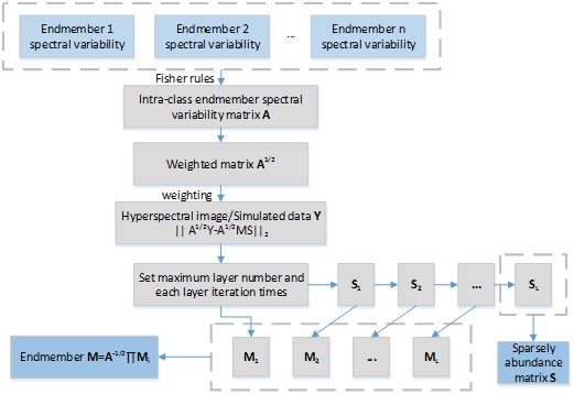
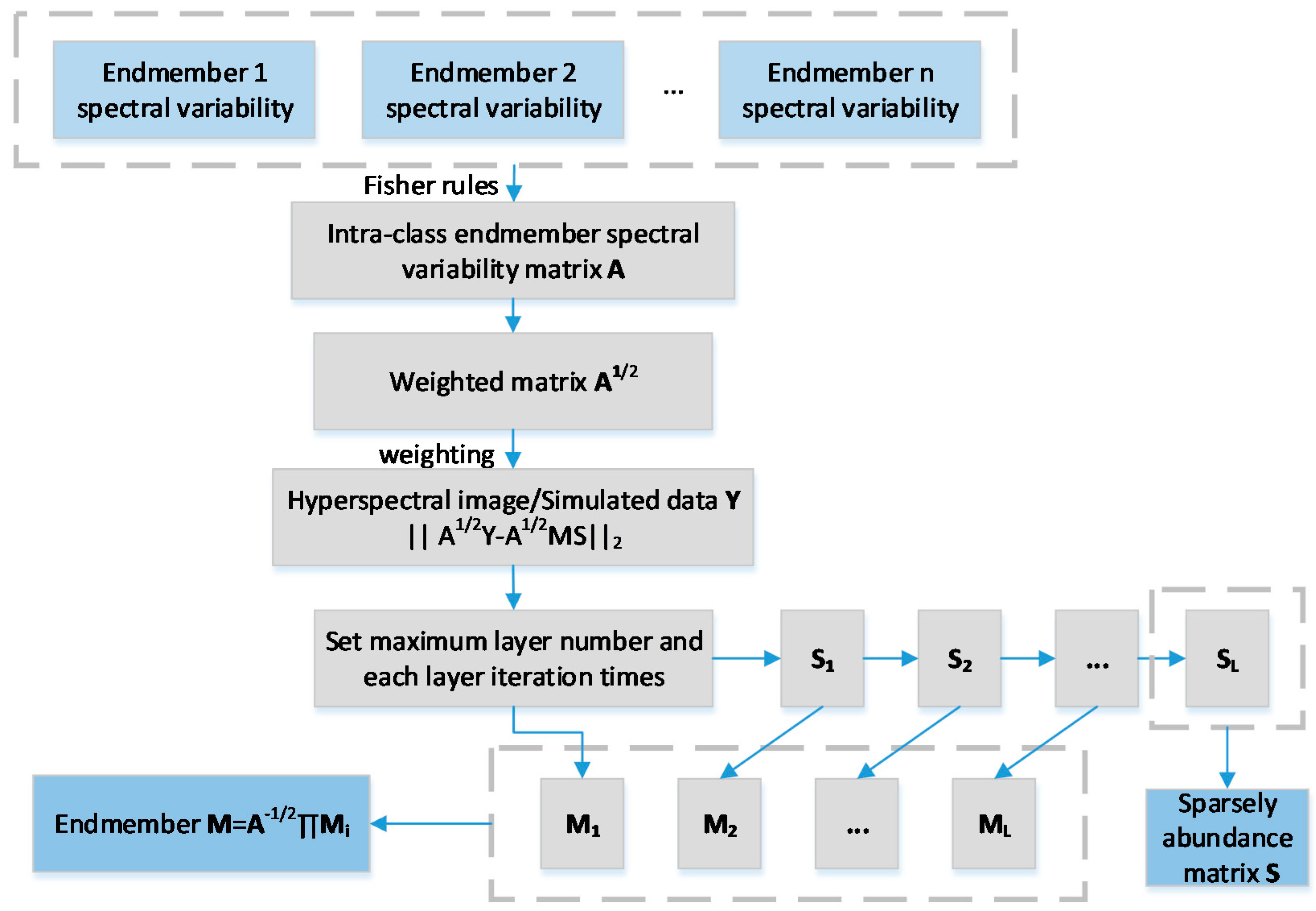
The amount of research has been developed in hyperspectral unmixing. Mixed pixel signals are generally modeled using linear or nonlinear mixing model. As a rule of thumb, the linear mixing model is associated with mixtures for which the pixel components are homogeneous surfaces in spatially segregated patterns. On the contrary, the nonlinear mixing model takes the intimate association or interaction with more than one component into account. The question of whether linear or nonlinear mixing model processes hyperspectral unmixing effectively is still an unresolved matter. Nevertheless, for many problems, the linear mixing model is thought to provide better accuracy in HU. The reason for this is due to the linear mixing model being computationally simpler than the nonlinear model. In this paper, on the basis of the linear mixing model, a hierarchical sparsity unmixing method is proposed and the schematic overview of the proposed method is shown in Figure 1.
2.1. Linear Mixing Model
When using the linear mixing model, the following three assumptions should apply: (1) the spectral signals are linearly contributed by a finite number of endmember within each IFOV weighted by their covering percentage (abundance); (2) the land covers are homogeneous surfaces and spatially segregated without multiple scattering; and (3) the electromagnetic energy of neighboring pixels does not affect each other [22,23,24]. Under the linear mixing model assumption, we have the equation below.
where M = [m1, …, mp] is the matrix of endmembers (mi denotes the ith endmember signature, l denotes the band number, and p is the number of endmembers). S is the abundance matrix ([S]i,j, which denotes the fraction of the ith endmember of the jth pixel and n denotes the total number of pixels) and . denotes a source of additive noise. The abundance matrix needs every element within it to be non-negative and the sum to be one in each column.
Y = MS + ε
2.2. Band Selection and Spectral Smoothness
For the hyperspectral unmixing, dimension reduction is not a necessary step. Experimental results from Li showed that while the feature extraction methods reduced the dimensionality of hyperspectral data and expedited subsequent processing, they did not help improve the accuracy of abundance estimations [25]. In contrast, Chang proposed a method of constrained band selection and a band-decorrelation approach for hyperspectral imagery to improve the classification accuracy. However, it should be noted that the accuracy of unmixing is mainly influenced by spectral variability [17]. The intra-class variability is linearly and negatively correlated with the accuracy of abundance fraction estimation provided by the least square spectral unmixing. In addition, the similarity between different types of endmembers may generate a high correlation between the columns in the endmember matrix, which, in turn, may lead to an unstable inverse matrix and a dramatic drop in estimation accuracy [26,27,28]. In other words, to improve the compactness and wellness of the endmember and abundance map, we need to enlarge the separation between endmember spectra and shrink the variances of residuals. In this paper, instead of reducing the image dimension, we remove the atmospheric water vapor absorption noise band. Spectral weighting will be introduced in the next section.
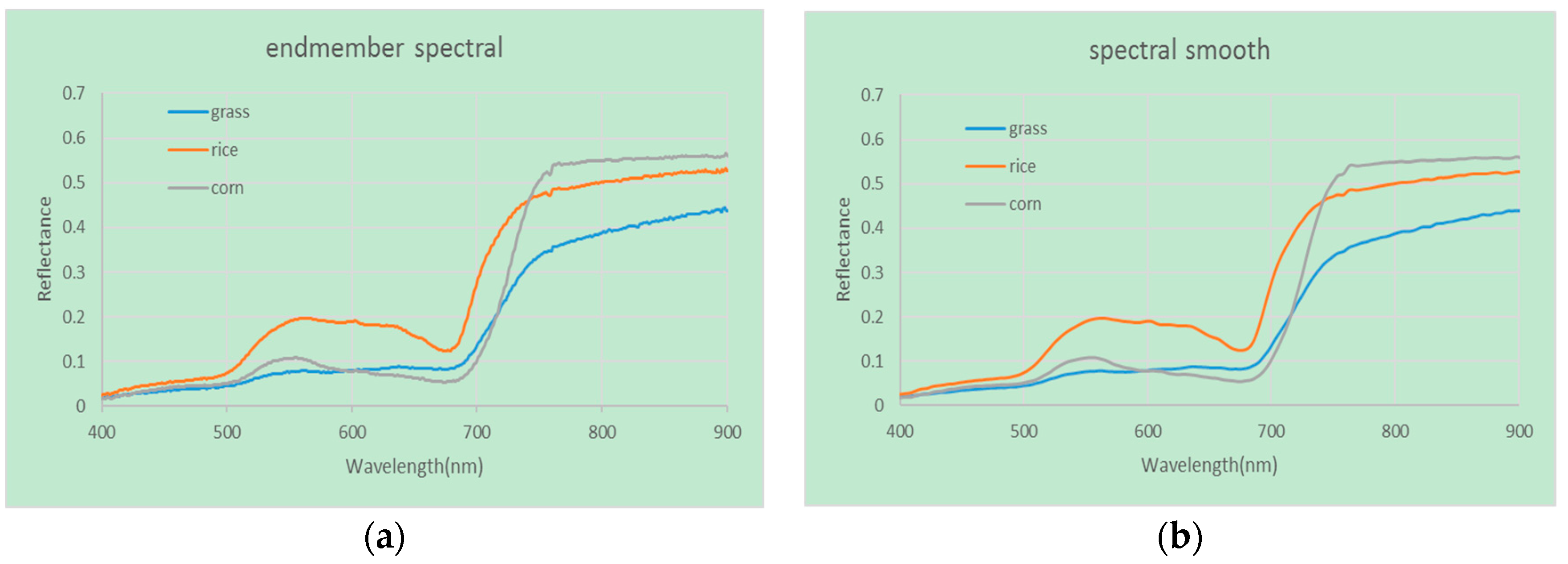
Since both the handheld and imagery spectral signal are sensitive to the noise, Savitzky-Golay smoothing filter [29] is used in this paper to remove the high-frequency noise.
2.3. Hierarchical Sparsity Constrained Unmixing
We adopt an interactive framework to extract the image endmember by combining the prior field knowledge with spectral analysis. Due to the effects of variable illumination and other conditions, the spectra captured by hyperspectral imaging illustrate spectral variability, which reduces the accuracy of hyperspectral unmixing. When it comes to distinguishing the similar endmembers such as the discrimination between the corn and weed, this becomes a difficult task. This is because some spectral variability of corn may be easily turned into a spectrum that is highly similar to the weed spectra. Therefore, a weighting spectral method considering the spectral variability is proposed to emphasize the separation of the similar spectrum and to improve the accuracy of the unmixing result.
Generally, to obtain M and S of the model in (1), it can be performed by minimizing the difference between Y and MS with the non-negativity constraint on M and S, respectively. The loss function based on the Euclidean Distance is interpreted in the equations below.
In particular, a simple additive update for S that reduces the squared distance can be written as
where the denotes the learning step, and is defined as
If is equal to some small positive number, the equation is equivalent to conventional gradient descent. Lee and Seung derived a multiplicative update rule in which the convergence was proven [30]. They set the , then the additive update rule of the abundance matrix could be turned into the multiplicative update rule. Likewise, the endmember matrix could also be achieved by modifying multiplicative update rules below.
According to Equation (2), the Euclidean Distance error is equally weighted for all bands, which assumes to have uniform effects. In general, this may not be necessarily true since the experimental results have demonstrated that the weighted spectral unmixing methods generally perform better than the traditional unweighted approaches [18]. Therefore, in this paper, a weighted matrix A is brought into Equation (2) so that the equation can be rewritten as the equation below.
where A is the diagonal elements of the within-class matrix defined by Fisher. Assuming that there are n training sample spectral vectors given by for p-class classification. with denotes the number of training sample vectors in the jth class and is the mean value of training samples. Then A is a positive-definite and symmetric matrix. Clearly, the earlier version (2) is seen in particular cases where the weighted matrix is chosen to be the identity matrix. A scale factor is also needed to enlarge the weighting of different bands. In order to turn the equation into non-negative matrix factorization form, we can use , the square-root form of A, and Equation (8) can be written below.
Except for the endmember spectral variability, we also put the sparsity constraint as a part of objective function for our minimization problem. Note that sparsity constraints have been widely used as an effective tool for hyperspectral unmixing [31]. Therefore, the objective function is combined within class spectra constraints, which enlarge the difference of different endmembers and decrease the variability of intra-class endmember spectra and abundance sparsity constraint. The objective function is defined below.
To improve performance in solving Equations (8) and (9), especially for ill-conditioned or badly scaled data and reducing the risk of getting stuck in local minima of a cost function, we develop a hierarchical procedure in which we perform a sequential decomposition of non-negative matrices for hyperspectral unmixing. The mathematical representation of hierarchical structure is formulated in the equation below.
where the L denotes the layer number. In each layer, the iteration can be updated through the equation below.
To avoid getting stuck in local minima, we defined the value of the parameter below, which is motivated by a temperature schedule in the simulated annealing technique.
where and are constants to regulate the sparsity constraints and denotes the iteration number in the process of optimization [32]. In each layer, the algorithm will be stopped from either meeting the maximum number of iterations or reaching the stopping criteria of the successive iterations. To accelerate the algorithm, we use Vertex Component Analysis (VCA) as the initial endmember and Fully Constrained Least Square (FCLS) to estimate the abundance matrix set [33]. The reason why using VCA as the initial set is that VCA is a prevalent fast algorithm in hyperspectral unmixing. And through the initial set, we can obtain more accurate results than the random initial set at the same number of iterations.
The flowchart of the proposed method is shown in Figure 2.
3. Data Acquisition for Verifying the Experiment
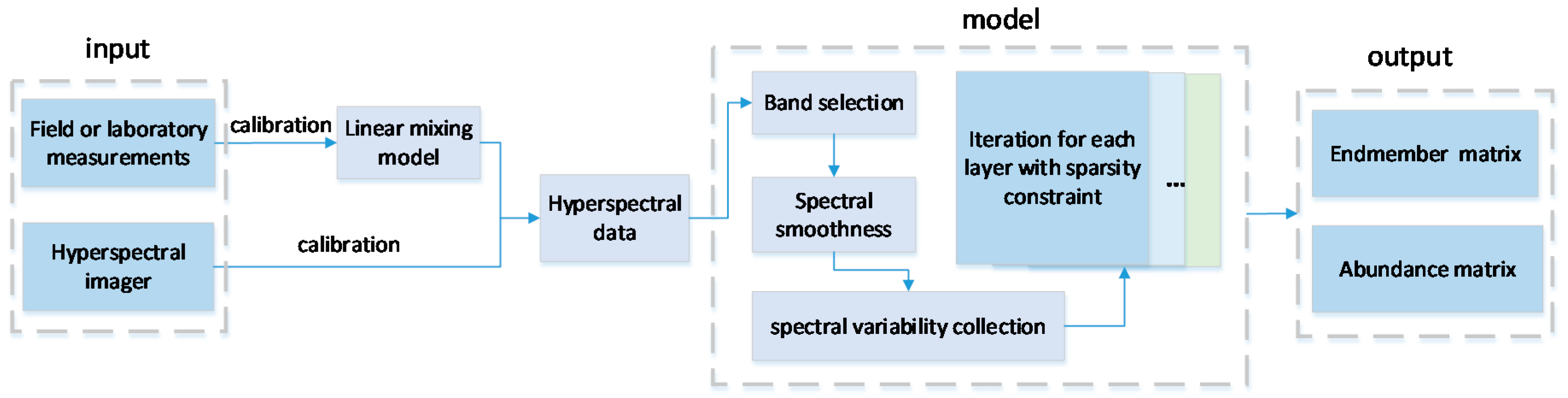
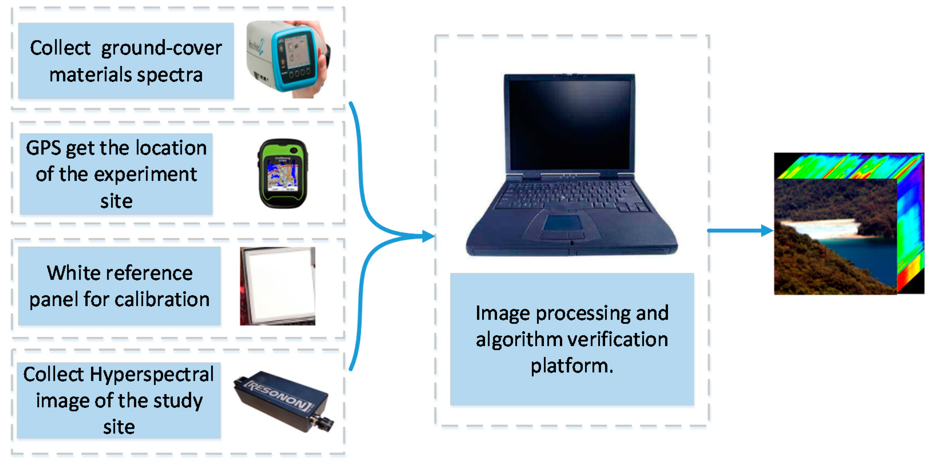
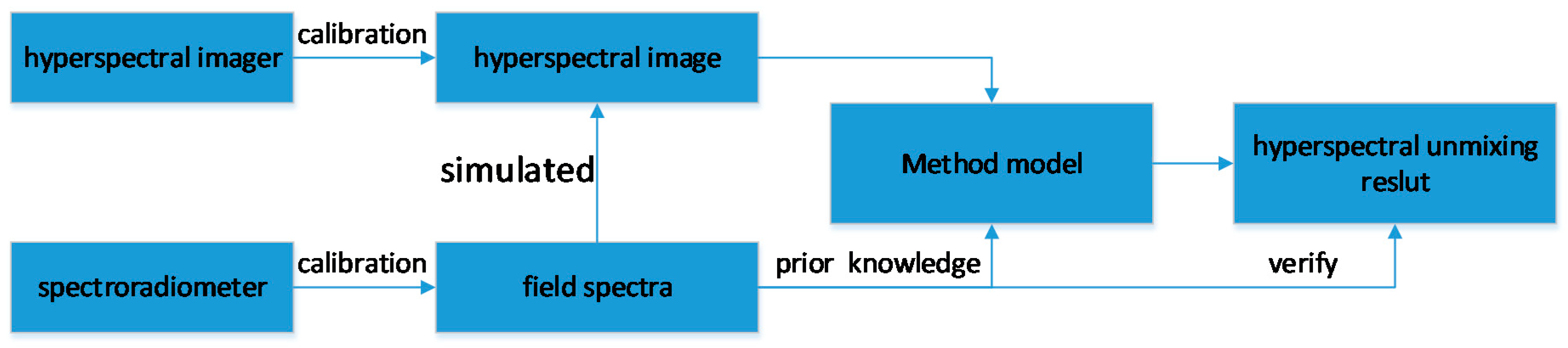
In general, experiments of linear unmixing can be verified by two types datasets, which include the simulated image data and the real hyperspectral image data. To verify the effectiveness of the proposed method, we investigate the study site and obtain in situ spectra and hyperspectral image. The geographic information was recorded by GPS. The system of the data acquisition is shown in Figure 3 and the data flow is illustrated in Figure 4.
3.1. Study Site and Ground Data Collection
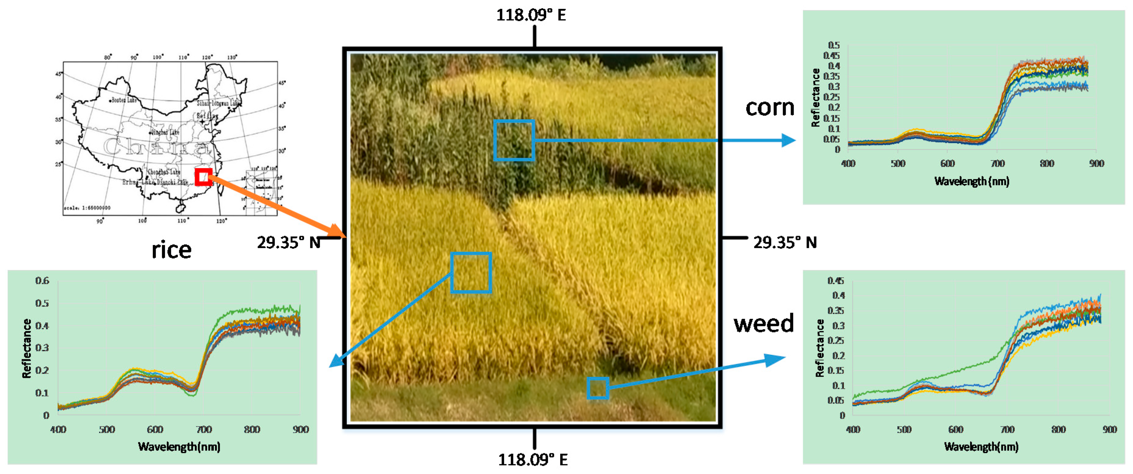
Our proposed method aims to improve the accuracy of endmember abundance fraction estimation due to the effect of spectral variability. The study site is located in the Jiangxi province. The first site named Data 1 is near Wuyuan, (29.35°N; 118.09°E), dominated by the rice, soft soil, corn, cedar, and water. The ground-cover materials spectra were measured using the FieldSpec Handheld2 Spectroradiometer of Analytical Spectral Devices (ASD) with 751 bands. The ASD has an ability to measure the electromagnetic radiance ranging from 325 nm to 1075 nm with an average spectral resolution superior to 3 nm. The ground-cover material spectral measurements were calibrated using a white reference panel with nearly 100% reflectance at all wavelengths every few minutes to ensure the accuracy of measurement results. Additionally, each sample was repeatedly measured 10 times with the spectroradiometer. The distance between the spectroradiometer and the sample was about 0.5–1.0 m to allow a target area radiance measurement. All sample spectra were measured at the nadir direction of the radiometer with a 25° field of view. Figure 5 shows a study site of Jiangxi where the situ contains rice, corn, and weed.
3.2. Image Acquisition and Preprocessing
The synthetic image is generated according to the linear mixing model based on Equation (1). The endmember can be obtained from the field or library spectra. The original field spectral data obtained by ASD is 751 bands. However, due to the decreased spectral sensitivity of the sensor at the two ends of the spectral range and due to the atmospheric water vapor absorption, bands 1–76 and 576–751 are blurred. Therefore, the final simulated data set is 499 spectral bands with the wavelength ranging from 400 nm to 900 nm. After determining the endmember matrix, we generate the abundance matrix randomly. In addition, a low pass filter is used to make the abundance variation smoother. To ensure that no pure pixel is present, all the abundance fractions larger than 0.8 are discarded. The synthetic image data set has size n = 3364 pixels. To make the scenes more realistic and reasonable, zero-mean white Gaussian noise is added and the signal-to-noise ratio (SNR) is set to 20 dB.
where E[·] denotes the expectation operator and the M and S matrix parameters are defined in Equation (1).
The real experimental data was captured by Pika XC2 imaging of Resonon, which is a push broom imager designed for the acquisition of visible and near-infrared hyperspectral imagery ranging from 400 nm to 1000 nm with 1.3 nm spectral resolution in September 2017. The second site, which is named Data 2, is shown in Figure 6. The image has 462 channels. Note that channels 1–13 and 385–462 were blurred due to the sensor noise and atmospheric water vapor absorption. As a result, we only used channels 13–384 with the wavelength ranging from 400 nm to 900 nm. Therefore, the final real experimental data is 372 bands. The image was calibrated using a white reference panel and converted from radiance to reflectance.
4. Experimental Results and Analysis
To illustrate the accuracy of unmixing results, spectral measurements are used in this paper. The results are evaluated using the spectral angle distance (SAD), the abundance angle distance (AAD), and the root mean squared error (RMSE).
SAD is defined by the equation below.
where mi denotes the ith endmember spectrum, 〈mi, mj〉 denotes the inner product of the two spectra, and denotes the vector magnitude. It is used to compare the similarity of the original pure endmember signatures and the estimated ones.
AAD is used on condition that the abundance fractions are known as prior knowledge. It measures the similarity between original abundance fractions (si) and the estimated one (), which is formulated in the equation below.
RMSE is denoted by
where N denotes the total number of pixels, l denotes the total number of spectral bands, and denotes the error of the ith row and the jth column between the original and simulated image data. It is used to evaluate the abundance estimates’ error. Since the model errors are likely to have a normal distribution rather than a uniform distribution, the RMSE is a good metric to present model performance [34].
4.1. Simulated Data Experiments
Providing the sub-pixel fraction abundance map of the image’s components is nearly impossible, expensive, and time-consuming. However, the simulated data makes it possible to preset the endmember set and the abundance fraction map as prior knowledge.
In this paper, several scenarios and patterns have been designed to evaluate the performance of the proposed method. In addition, different signal-to-noise ratios have been employed to generate the simulated images.
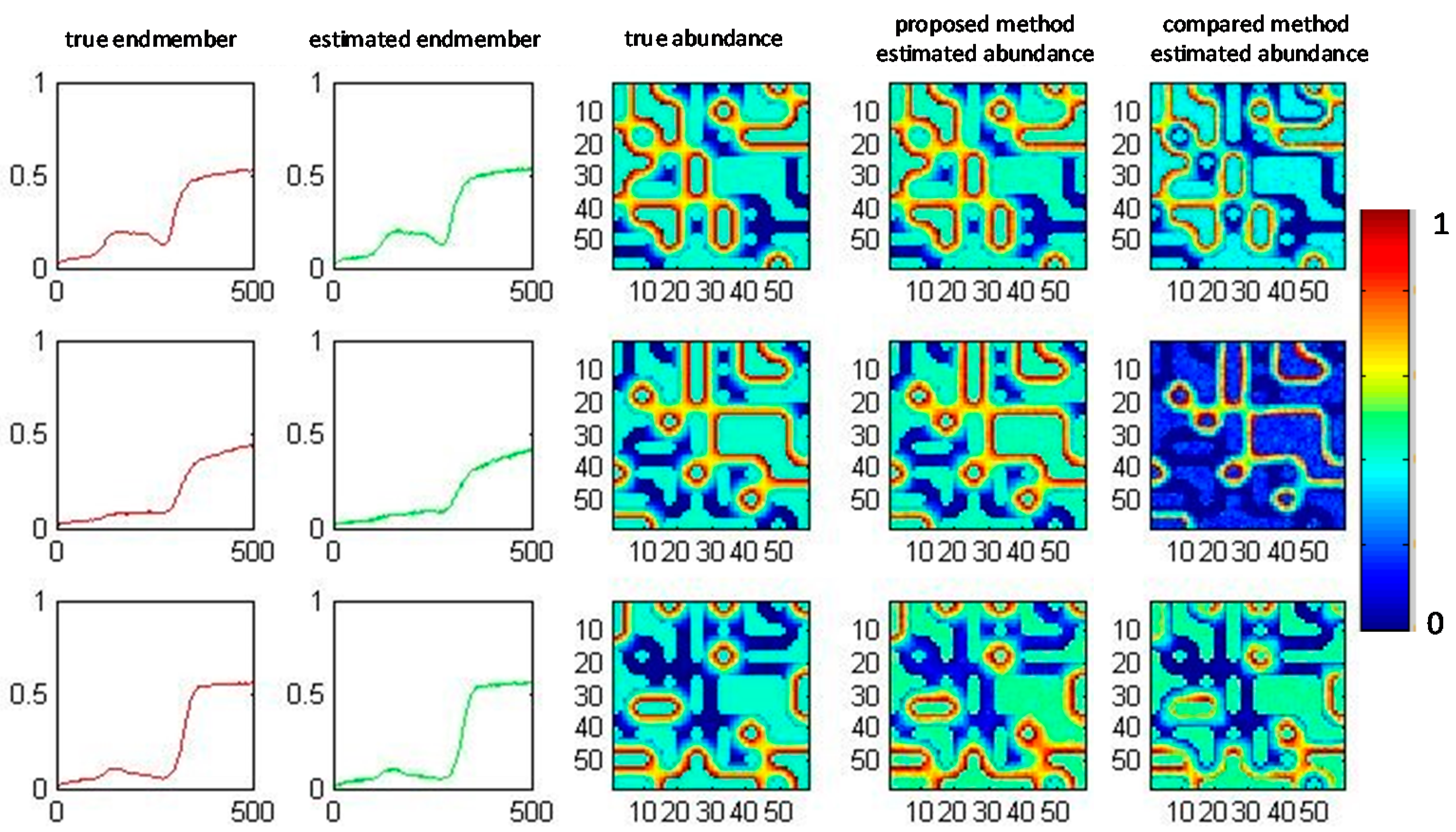
4.1.1. Synthetic Data Experimental Results
In the first experiment, the endmembers are rice, corn, and weed and the SNR is set to 20. The layer number is 5 and the maximum iteration times in each layer is 1000. Furthermore, we set Figure 8 shows the unmixing results of the proposed method and the non-weighted L1/2 sparsity constrained NMF (L1/2S-NMF) method [31]. Among them, the first column is the true endmembers spectra and the second column is the estimated endmembers spectra by the proposed method. The third column is the original abundance map and the last two columns are the estimated abundance map by the proposed method and comparison method, respectively. The abundance fraction map is denoted using a color bar showing color scale. The blue color shows the smallest fraction near zero and the red color shows the highest fraction near one. The variation of the color bar is consistent with the natural spectral wavelength change. Through the comparison, it can be seen that the proposed algorithm performs better than the comparative method especially in the weed abundance fraction estimation. This is because the similarity among the crops and weed is difficult to distinguish by the traditional method, which the crops and weed cannot be the vertices of any convex simultaneously.
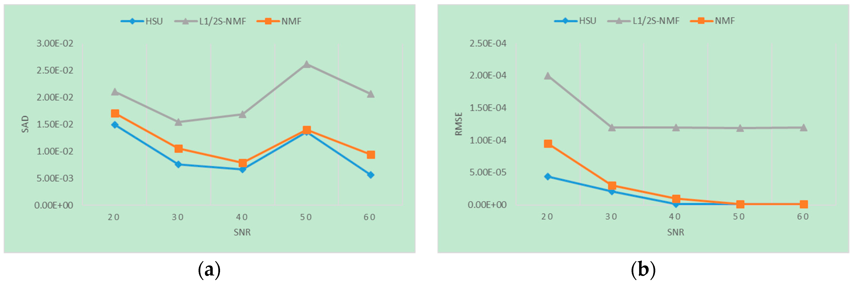
4.1.2. Influence of SNR
The second experiment presented there aims at evaluating the performance of the methods with different SNR. The SNR varies from 20 to 60. The endmember number is 6. Figure 9 is the SAD and RMSE accuracy assessment results of the proposed algorithm, NMF, and L1/2S-NMF. Since the scenarios and patterns of the simulated datasets are randomly generated, it is a good approach to evaluate the goodness and stability of unmixing results by different methods.
From Figure 9, with the increase of the SNR, there is also a decrease of the estimated RMSE errors for all methods while the proposed method shows clear advantages. It should be noted that in Figure 9a, there is a small increase of SAD where the SNR is 50. That is due to the fact that the simulated image abundance is a random series that may produce highly mixed data. However, under this condition, the proposed method still outperforms more than other approaches. Therefore, combining intra-class scatter matrix information with hierarchical sparsity constrained NMF, the proposed algorithm can obtain a good performance in hyperspectral unmixing.
4.1.3. Influence of Layer Number and Endmember Number
To verify how the layer and endmember number affect the proposed method in hyperspectral unmixing accuracy, we experiment with various layers and endmembers under the same fixed initial condition. In this experiment, the endmember number is set from 4 to 12 and the number of layers varies from 1 to 16. It should be noted that the endmember number is known as prior knowledge and the other parameters such as SNR and the total number of iterations keep invariant than previously mentioned. The initial endmember and abundance matrix are extracted by VCA-FCLS, which are the input of the proposed method with different layers. Therefore, with the fixed dataset and initial input parameters, the influence of layers and endmember number on unmixing results can be observed. It is worth mentioning that, when the layer number is one, it can be approximately regarded as the single layer sparsity-based NMF method. We also make a comparison with L1/2S-NMF. The parameter of L1/2S-NMF is set the same as mentioned in the literature [31]. The results are shown in Table 1. The best accuracy results with different endmember numbers are in bold fonts. From the table, it can be inferred that the best choice of the layer number setting is approximately linear with the endmember number. The AAD accuracy is increased with the layer number. It is true that the error of the hierarchical system may be accumulated layer by layer. However, the AAD error can still be controlled to a degree. The proposed method still outperforms when the method is compared against various endmember numbers.
4.1.4. Influence of Iterations
In this experiment, we intend to find the number of iterations’ effect on final unmixing accuracy. We still fix the initial endmember set. The endmember and layer number are set to 8 and 10, respectively. The iteration in each layer varies from 100 to 3000. Additionally, the other parameters such as lambda or SNR keep invariant. The accuracy results are shown in Table 2. As expected, the best performance regarding of AAD and SAD is obtained with the larger iteration number. Note that there exists a balance between the maximum layer number and accuracy. When the number of iterations ranges from 100 to 200, the accuracy increases drastically. When the number ranges from 400 to 1000, the accuracy increases linearly. Whereas when the iteration number is larger than 1000, the rate of convergence slows down and becomes flat. This is due to the fact that the algorithm converges gradually and has reached the stopping criteria before getting the maximum iteration number. Generally, the number of iterations in each layer is set to 2000.
4.1.5. Time-Consuming with Layer Number
Finally, to conclude this section, we emphasize the computation complexity of the hierarchical sparsity unmixing method considered in this study. For the proposed method, the computational complexity is approximately given by the product of the computational complexity of each layer and the number of iterations. In this experiment, there are 58 × 58 pixels and the endmember number and SNR are set to 8 and 25, respectively. Furthermore, the regularization parameters and the whole iterations keep invariant. The time-consuming results versus the layer number is shown in Table 3. Through the results, it can be concluded that, as layer numbers increase, better performance in saving time is shown. This is due to the hierarchical strategy breaking the large matrix into two parts. In the traditional NMF with single layer, the computational cost in one iteration is . However, in the hierarchical strategy, the computational cost in one iteration of the second or latter layer is . Additionally, the value of p is less than L. Consequently, it can be inferred that the performance of the hierarchical algorithm in the saving time-consuming process is substantially better than the traditional single layer NMF.
To summarize, the results mentioned above confirm the satisfactory performance of the proposed method in terms of unmixing quality and computational time. The best results are obtained with a proper layer number. Additionally, the proposed method is robust to the different conditions that can affect hyperspectral images.
4.2. Real Hyperspectral Data Experiments
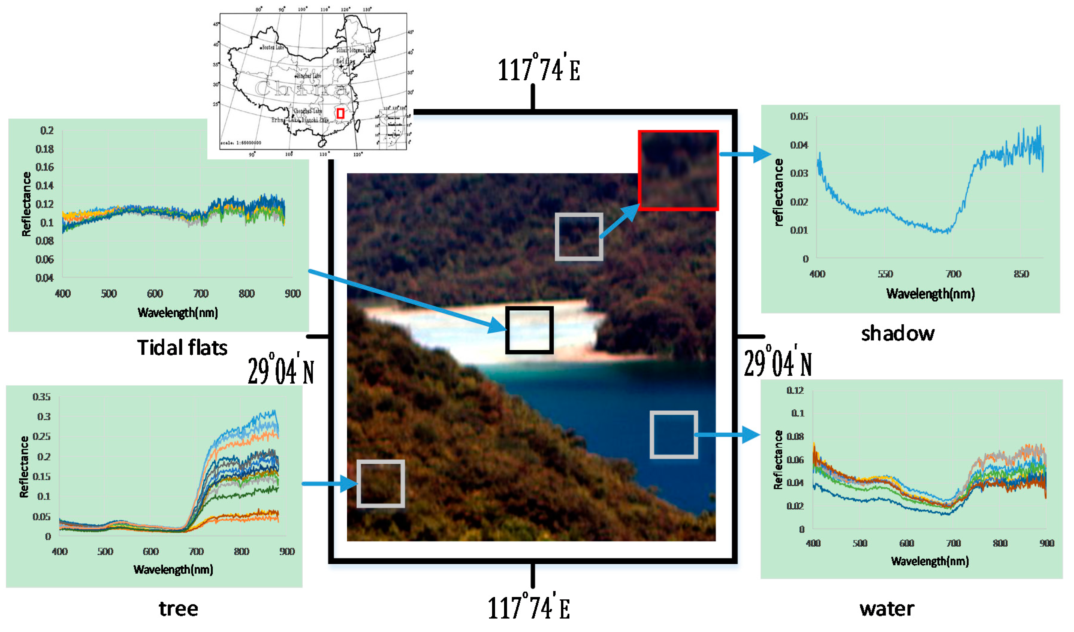
In this section, we use two different scenarios to verify the effectiveness of the proposed method. The images are collected in Jiangxi captured by Pika XC2 imaging of Resonon. We choose 90 pixels with 30 pixels for each endmember directly from the image. Then an average of the observations in each endmember class is computed, which serves as the reference endmember spectra. Additionally, each endmember spectral class can be served as a weighted matrix to reduce endmember variability effect. The size of the test image is 400 × 400 × 372. Figure 6 shows the other study site of Jiangxi. There are tidal flats, tree, and water in the scene. From the image, it should be noted that on the top right of the spectrum, the shadow among the tree canopy is similar to the water spectrum to some degree. However, in the near-infrared wavelength, the shadow spectrum reserves the property of red edge, which is unique for plants. In other words, except for the similarity of interclass endmember spectra, there also exists intra-class spectral variability. Therefore, the spectral variability of both interclass and intra-class increase the difficulty of hyperspectral unmixing. In this paper, we use the intra-class scatter matrix weighted constraint to decrease the intra-class endmember variability and enlarge the interclass spectral variability. The endmember and layer number is set as 3 and 5, respectively. The iteration in each layer is set to 1000.
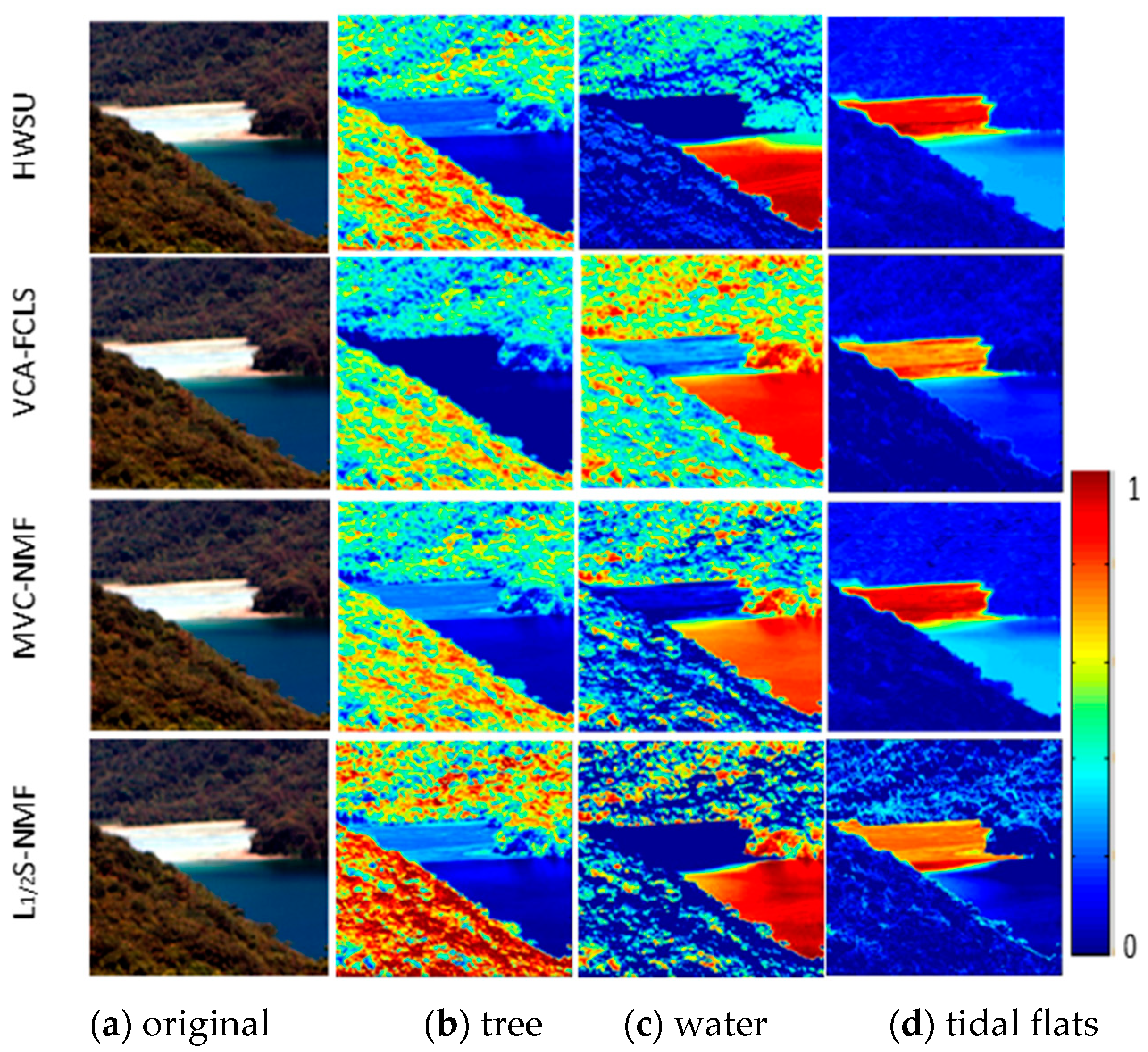
Figure 10 is the unmixing results of the proposed method and the traditional method. The compared methods are geometric-based VCA with fully constrained least square (FCLS) [33], minimum volume constrained non-negative matrix factorization (MVC-NMF) [35], and sparsity constrained non-negative matrix factorization (L1/2S-NMF) [31]. Since the weeds and crops have highly similar diagnostic spectral features, the rice, weed, and corn in Figure 10 are not the vertices of any convex set. Therefore, they cannot be endmember sets simultaneously in the geometric simplex [22]. This is why the traditional unmixing method such as VCA-FCLS and MVC-NMF cannot distinguish them effectively. Note that in Figure 10c,d, the wrong estimation of weed and corn is good evidence to illustrate this phenomenon. On the other hand, the proposed method takes the intra-class endmember variability into account and through the difference within endmember spectral, we make a weighting for each band. Furthermore, a hierarchical sparsity strategy is also used to search the optimal global solution. Then we can obtain a better result than the traditional one especially in distinguishing the corn and weed.
From Figure 11, it can be seen that, in the tree canopy and beach abundance fraction maps, the proposed method estimates better than the traditional method, which is more close to reality. On the water abundance map, all the methods have little error that the shadow of the tree canopy shows the higher faction in these maps. This is due to the fact that the shadow spectra show lower magnitude, which is similar to the water feature. However, it is worth mentioning that the proposed method has a better ability to circumvent the shadow effect than the traditional approach to distinguish these spectra. Table 4 and Table 5 illustrate the mean SAD and RMSE accuracy of different algorithms. The lower SAD and RMSE shows the better estimation of reconstructed data. Both the results show that the proposed method can obtain the best result of all.
Based on the real hyperspectral image captured by Pika XC2 imaging of Resonon, the most of the endmember variability can be interpreted by a variation in illumination, which is mainly located in vegetation areas and among trees. Experimental results show that it is feasible to combine the spectral weighted matrix with hierarchical strategy in reducing the spectral variability effect on unmixing accuracy. Furthermore, the proposed method also outperforms the compared methods.
4.3. Potential Applications
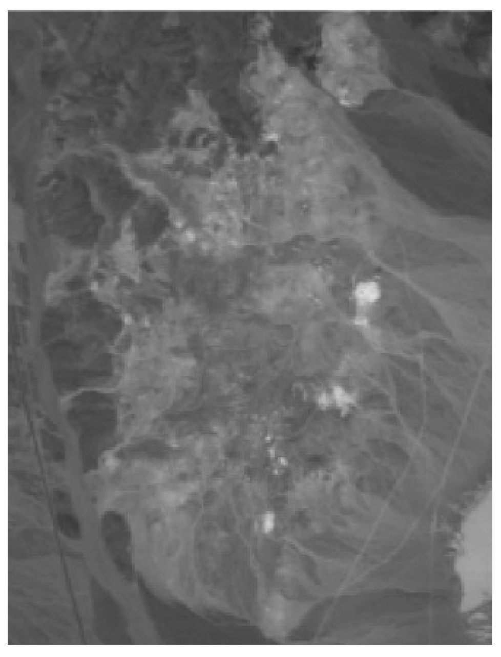
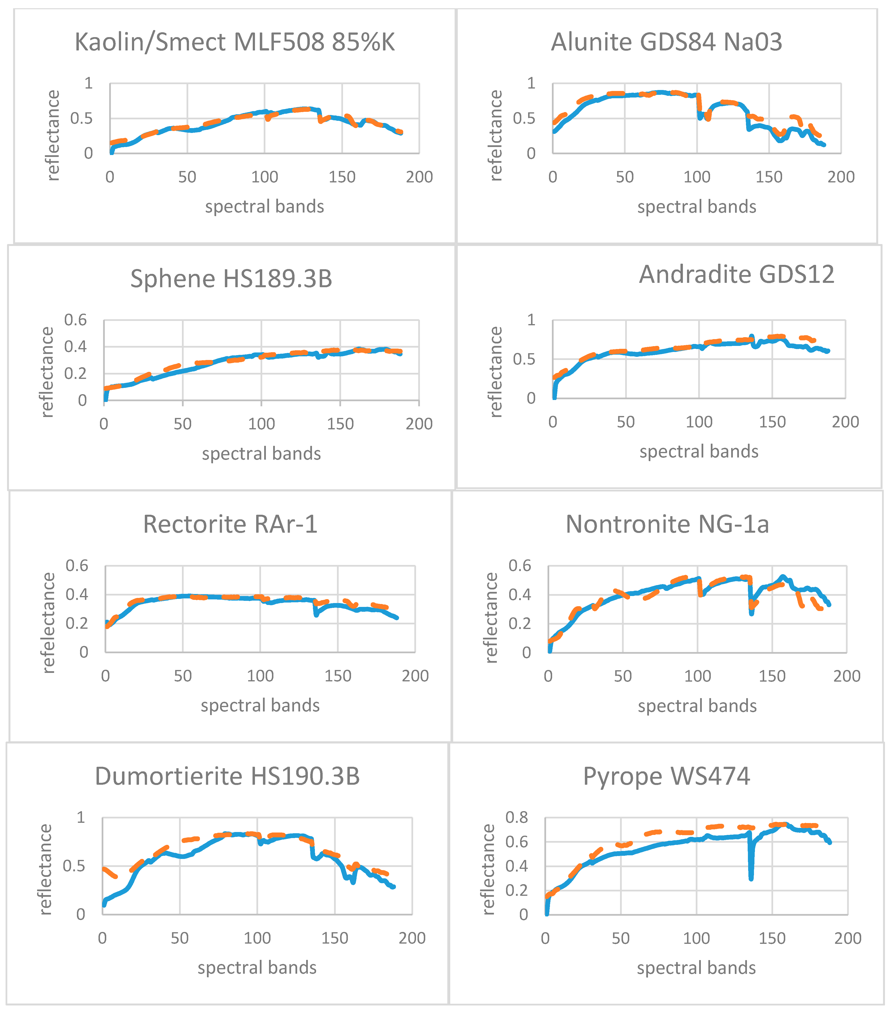
In this experiment, we use the classic hyperspectral image, named Data 3, to illustrate the performance of unmixing methods. The image is captured by Airborne Visible-Near infrared Imaging Spectrometer (AVIRIS) hyperspectral sensor, which is shown in Figure 12. It is located at Cuprite, Nevada USA. The original data has 512 × 614-pixel with 224 bands. The wavelength ranges from 400 nm to 2500 nm, full width at half maximum of 10 nm, and the spatial resolution is 20 m. We use the sub-image data with size 250 × 191. After removing low SNR and water-vapor absorption bands (1–2, 104–113, 148–167, and 221–224), 188 bands are remained. The situation is located in Cuprite Nevada, which is a mineralogical site that has been established as a reference site for hyperspectral and other remote sensing instruments [36,37,38]. Cuprite is an arid and sparsely vegetated place along the California-Nevada border near Death Valley. It contains sulfates (K-Alunite, Jarosite, etc.), Kaolinite group clays (Kaolinite, Dickite, etc.), Carbonates (Calcite, Calcite+montmorillonite), Clays (Na-Montmorillonite), and other minerals. Since the spectral variability matrix is hard to obtain from the image, we define the weighted matrix as the unit matrix. According to the reference [31], we set endmember and layer number as 10 and 8, respectively, and part of unmixing results are shown in Figure 13. The blue solid lines illustrate the original spectra from the USGS library and the orange dotted lines are spectra extracted by the proposed method. Clearly, the endmember spectra extracted by the proposed method are in good accordance with USGS library. Table 6 and Table 7 show the SAD and RMSE accuracy generated by the proposed method and compared ones, which are L1/2S-NMF and VCA, respectively. It can be seen that the proposed method can extract better endmember and abundance estimation results versus the traditional approaches.
Results from Cuprite data confirms that the proposed method can extract different endmember signatures in the observed scenes accurately without weighted spectral variability matrix.
5. Discussion
As summarized in published research [39,40], hyperspectral unmixing approaches can be categorized into geometric, statistical, and sparse regression-based algorithms. To some degree, the proposed method is closely linked to the minimum volume method through its geometric interpretation, which is easy to understand. It is intuitive because if the volume of simplex becomes large, the observed pixels become less sparse [31]. Additionally, through the abundance sparsity constraint, the abundance maps can be more accurately recovered.
From the experimental results, several issues should be noted. First, endmember spectra from the field can be controlled well and measured accurately, but they may not match those in the image due to differences in sensors, atmospheric effects, and illumination conditions. This is the reason why it is impossible to obtain the same high accuracy result of simulated data and real hyperspectral data. Furthermore, linear mixing model excludes the nonlinear effects caused by the complex canopy structures and possible multi-reflection effects. The combination of the intra-class scatter matrix endmember spectra in a single analysis improved the accuracy of similar terrain covering endmember spectral extraction and abundance estimation in each scenario.
Second, for all scenarios and all noise levels, the traditional linear unmixing methods provided the least accurate abundance fraction estimates. As commonly accepted, this is due to the high similarity between the weed and crops spectra, which is evident from Figure 7 and intra-class spectral variability. This results in unstable model inversion. Using a weighted matrix makes it possible to enlarge the separation between endmember spectra and shrinks the variances of residuals. On the other hand, the selection of lambda is also an open theoretical issue. In the research [41], it sets the lambda value based on the sparseness criteria, which is highly dependent on the sparsity of the material abundances. In addition, the method is widely used in other unmixing methods [31]. However, in this paper, we refer to the research [32] to define the value of lambda. Additionally, through the experimental results, it outperformed traditional sparsity criteria in the hierarchical sparsity constraint unmixing method.
Third, it is an open theoretical issue to prove mathematically or explain more rigorously why the hierarchical or multilayer distributed NMF system results in considerable improvement in performance and reduces the risk of getting stuck in local minima. An intuitive explanation is that the multilayer system provides a sparse representation of basis matrices Mi. In other words, even a true basis endmember matrix is not sparse, it can still be represented by a product of a sparse factor. Furthermore, experiments have shown that using hierarchical sparsity strategy can considerably improve the performance especially if a problem is ill-conditioned or data are badly scaled and projected gradient algorithms are used [32].
Fourth, the fittest layer number to obtain the best accuracy results needs to be further researched. Take the Section 4.1.3 simulated experiment with specific 10 endmembers as an example. We have conducted the experiments at least 120 times with the weighed matrix as the unit matrix. In each synthetic data, the best SAD accuracy with layer number was counted. From the result, it indicated that the fittest layer number for the SAD result might be 12, which has got 24 times among the 120 kinds of synthetic data. Then it might be 22, 30, and 16. All of them are larger than the endmember number. It seems that the fittest layer number are more likely larger than the endmember. However, it should be noted that when the layer number is too big, it may raise errors in abundance estimation, which is mentioned in Section 4.1.3. On the contrary, we also conducted the similar experiment with eight endmembers. And compared with 10 endmembers, there is a big probability to get the best results in eight and five layers, which are equal to or a somewhat smaller than the endmember number. The other relationship between the endmember number and the layer number is analogous to this condition. Furthermore, the results of the other layer number are also acceptable even though they are not the optimal solution. Therefore, when it comes to determining the layer number, a value ranging from 0.5 to 2 times of the endmember number may be a good choice.
Fifth, when it comes to selecting a methodology to apply, an important aspect that end-users always take into account is how feasible it is to quickly apply the methodology, how many input parameters are involved, how difficult it is to set them to obtain appropriate results, how much prior knowledge is needed in order to run each technique, and what the main caveats are when running the algorithms [7]. This paper uses the field or laboratory spectra to estimate the similarity endmembers’ abundance and the model is easy to understand. If it is hard to obtain field spectra for establishing a weighted matrix of endmember variability, this information could be directly extracted from the image. Through the visual observation and prior knowledge, we can choose the specific area of the image to extract spectra as a reference spectral matrix. Note that the endmembers extracted from the image have an advantage over library or field endmembers because they are collected under nearly the same conditions as the image. In this way, we can both obtain the reference endmember matrix and the weighted matrix. Furthermore, the input parameters are also simple to implement. The effectiveness of the proposed method has been verified by the simulated and real hyperspectral image and the application can be expanded to monitor glacier or other applications. Superior to the supervised algorithm, the proposed method only uses the partial intra-class endmember similarity information to make a weighting on each band, which will enlarge the separation of similar spectra and to obtain better unmixing results. For another, if it is hard to obtain the intra-class endmember similarity information especially if there’s no prior knowledge at all. Yet, we can reset the weighted matrix as the unit matrix. Furthermore, the hierarchical non-negative matrix factorization has been proven effective and applied on signal processing and other areas [32]. Therefore, the proposed method can be applied on the other dataset. In addition, we intend to further stimulate efforts to merge the different conceptual approaches—iterative mixture analysis cycles, feature selection, spectral transformations, and spectral model—to reduce endmember variability effect and enhance unmixing accuracy.
6. Conclusions
Spectral variability has been under-researched in recent years. Experimental data were used to familiarize readers with the positive effects that endmember spectral variability reduction techniques can have on subpixel fraction estimate accuracy. However, in some environments or for some applications, similarities of different endmembers of interest provides an additional difficulty for obtaining accurate estimation or classification results. The weighted matrix makes it possible to emphasize the different bands in distinguishing similar endmembers. In addition, five basic principles aiming to reduce the spectral variability’s effect should also be considered. The integration of different methods is a prerequisite for the effective mitigation of endmember spectral variability.
This research took spectral variability into consideration to unmix hyperspectral images. We used field-measured or lab-measured spectra as prior knowledge and computed the within-class scatter matrix as a weighted matrix of the image. In contrast with previous supervised approaches, the proposed method only used the prior knowledge as each band’s weighted matrix rather than a fixed endmember input. In addition, the hierarchical sparsity is also considered and aims to obtain better unmixing results. Therefore, it is feasible to examine the suitability of unmixing results by comparing the different methods.
To verify the proposed algorithm, experiments with simulated and real-world hyperspectral image data were conducted. The spectral curves and abundance map results confirmed the effectiveness of hyperspectral unmixing (HU) particularly in the presence of noise corruption, low purity levels, and similar endmember conditions. Considering the RMSE, SAD, and AAD of the obtained abundance maps, the proposed HWSU method outperformed VCA-FCLS, MVC-NMF, and L1/2S-NMF and was compatible with the simulated and in situ observations.
Author Contributions
J.Z. and J.L. conceived and designed the study; J.Z. and Y.S. conducted the field experiments; J.Z. and J.L. analyzed the data. J.Z. processed the images, wrote and revised the manuscript. J.L. gave advice on the methodology and paper revision. Y.S. also revised the manuscript.
Acknowledgments
The work is supported by the Major Special Project of the China High-Resolution Earth Observation System. We would like to thank the editor and reviewers for their reviews that improved the content of this paper. And we also would like to thank Yuzhen Zhang of University of Science and Technology Beijing for giving valuable suggestions on paper revision.
Conflicts of Interest
The authors declare no conflict of interest.
References
- Bioucas-Dias, J.M.; Plaza, A.; Camps-Valls, G.; Scheunders, P.; Nasrabadi, N.; Chanussot, J. Hyperspectral remote sensing data analysis and future challenge. IEEE Geosci. Remote Sens. Mag. 2013, 1, 6–36. [Google Scholar] [CrossRef]
- Thomas, M.L.; Ralph, W.K.; Jonathan, W.C.; Peng, W.L.; Yu, X.C.; He, H.; Chen, H.S. Remote Sensing and Image Interpretation; Publishing House of Electronics Industry: Beijing, China, 2016; pp. 382–400. [Google Scholar]
- Halimi, A.; Honeine, P.; Bioucas-Dias, J.M. Hyperspectral unmixing in presence of endmember variability, nonlinearity, or mismodeling effects. IEEE Trans. Image Process. 2016, 25, 4565–4579. [Google Scholar] [CrossRef] [PubMed]
- Halimi, A.; Honeine, P.; Kharouf, M.; Richard, C.; Tourneret, J.-Y. Estimating the intrinsic dimension of hyperspectral images using an eigen-gap approach. IEEE Trans. Geosci. Remote Sens. 2016, 54, 3811–3821. [Google Scholar] [CrossRef]
- Thouvenin, P.A.; Dobigeon, N.; Tourneret, J.Y. Hyperspectral unmixing with spectral variability using a perturbed linear mixing model. IEEE Trans. Signal Process. 2016, 64, 525–538. [Google Scholar] [CrossRef]
- Ghaffari, O.; Zoej, M.J.V.; Mokhtarzade, M. Reducing the effect of the endmembers’ spectral variability by selecting the optimal spectral bands. Remote Sens. 2017, 9. [Google Scholar] [CrossRef]
- Somers, B.; Asner, G.P.; Tits, L.; Coppin, P. Endmember variability in spectral mixture analysis: A review. Remote Sens. Environ. 2011, 115, 1603–1616. [Google Scholar] [CrossRef]
- Costanzo, D.J. Hyperspectral imaging spectral variability experiment results. In Proceedings of the IEEE International Geoscience and Remote Sensing Symposium, Honolulu, HI, USA, 24–28 July 2000. [Google Scholar]
- Zare, A.; Ho, K.C. Endmember variability in hyperspectral analysis: Addressing spectral variability during spectral unmixing. IEEE Signal Process. Mag. 2014, 31, 95–104. [Google Scholar] [CrossRef]
- Drumetz, L.; Veganzones, M.A.; Henrot, S.; Phlypo, R.; Chanussot, J.; Jutten, C. Blind hyperspectral unmixing using an extended linear mixing model to address spectral variability. IEEE Trans. Image Process. 2016, 25, 3890–3905. [Google Scholar] [CrossRef] [PubMed]
- Zhang, J.; Rivard, B.; Sánchez-Azofeifa, A.; Castro-Esau, K. Intra- and inter-class spectral variability of tropical tree species at La Selva, Costa Rica: Implications for species identification using HYDICE imagery. Remote Sens Environ. 2006, 105, 129–141. [Google Scholar] [CrossRef]
- Nascimento, J.M.P.; Dias, J.M.B. Vertex component analysis: A fast algorithm to unmix hyperspectral data. IEEE Trans. Geosci. Remote Sens. 2005, 43, 898–910. [Google Scholar] [CrossRef]
- Li, J.; Bioucas-Dias, J. Minimum volume simplex analysis: A fast algorithm to unmix hyperspectral data. In Proceedings of the IEEE International Geoscience and Remote Sensing Symposium, Boston, MA, USA, 7–11 July 2008. [Google Scholar]
- Somers, B.; Zortea, M.; Plaza, A.; Asner, G.P. Automated extraction of image-based endmember bundles for improved spectral unmixing. IEEE J. Sel. Top. Appl. Earth Obs. Remote Sens. 2012, 5, 396–408. [Google Scholar] [CrossRef]
- Roberts, D.A.; Gardner, M.; Church, R.; Ustin, S.; Scheer, G.; Green, R.O. Mapping chaparral in the santa monica mountains using multiple endmember spectral mixture models. Remote Sens Environ. 1998, 65, 267–279. [Google Scholar] [CrossRef]
- Veganzones, M.A.; Drumetz, L.; Tochon, G.; Mura, M.D.; Plaza, A.; Bioucas-Dias, J.-M.; Chanussot, J. A new extended linear mixing model to address spectral variability. In Proceedings of the 6th IEEE Workshop on Hyperspectral Image and Signal Processing: Evolution in Remote Sensing (WHISPERS), Lausanne, Switzerland, 24–27 June 2014. [Google Scholar]
- Chang, C.I.; Wang, S. Constrained band selection for hyperspectral imagery. IEEE Trans. Geosci. Remote Sens. 2006, 44, 1575–1585. [Google Scholar] [CrossRef]
- Chang, C.I.; Ji, B. Weighted abundance-constrained linear spectral mixture analysis. IEEE Trans. Geosci. Remote Sens. 2006, 44, 378–388. [Google Scholar] [CrossRef]
- Zhang, J.; Rivard, B.; Sanchez-Azofeifa, A. Derivative spectral unmixing of hyperspectral data applied to mixtures of lichen and rock. IEEE Trans. Geosci. Remote Sens. 2004, 42, 1934–1940. [Google Scholar] [CrossRef]
- Wu, C. Normalized spectral mixture analysis for monitoring urban composition using ETM + imagery. Remote Sens. Environ. 2004, 93, 480–492. [Google Scholar] [CrossRef]
- Hong, D.F; Yokoya, N.; Chanussot, J.; Zhu, X.X. Learning a low-coherence dictionary to address spectral variability for hyperspectral unmixing. In Proceedings of the IEEE International Conference on Image Processing (ICIP), Beijing, China, 17–20 September 2017. [Google Scholar]
- Miao, X.; Gong, P.; Swope, S.; Pu, R.; Carruthers, R.; Anderson, G.L.; Heaton, J.S.; Tracy, C.R. Estimation of yellow starthistle abundance through CASI-2 hyperspectral imagery using linear spectral mixture models. Remote Sens. Environ. 2006, 101, 329–341. [Google Scholar] [CrossRef]
- Karnieli, A. A review of mixture modeling techniques for sub-pixel land cover estimation. Remote Sens. Rev. 1996, 13, 161–186. [Google Scholar]
- Keshava, N.; Mustard, J.F. Spectral unmixing. IEEE Signal Process. Mag. 2002, 19, 44–57. [Google Scholar] [CrossRef]
- Li, J. Wavelet-based feature extraction for improved endmember abundance estimation in linear unmixing of hyperspectral signals. IEEE Trans. Geosci. Remote Sens. 2004, 42, 644–649. [Google Scholar] [CrossRef]
- Settle, J. On the effect of variable endmember spectra in the linear mixture model. IEEE Trans. Geosci. Remote Sens. 2006, 44, 389–396. [Google Scholar] [CrossRef]
- Barducci, A. Theoretical and experimental assessment of noise effects on least-squares spectral unmixing of hyperspectral images. Opt. Eng. 2005, 44, 87008. [Google Scholar]
- Debba, P.; Carranza, E.J.M.; Meer, F.D.V.D.; Stein, A. Abundance estimation of spectrally similar minerals by using derivative spectra in simulated annealing. IEEE Trans. Geosci. Remote Sens. 2006, 44, 3649–3658. [Google Scholar] [CrossRef]
- Savitzky, A.; Golay, M.J. Smoothing and differentiation of data by simplified least squares rpocedures. Anal. Chem. 1964, 7, 1627–1639. [Google Scholar] [CrossRef]
- Lee, D.D.; Seung, H.S. Algorithms for non-negative matrix factorization. In PInternational Conference on Neural Information Processing Systems; MIT Press: Cambridge, MA, USA, 2000. [Google Scholar]
- Qian, Y.; Jia, S.; Zhou, J.; Robles-Kelly, A. Hyperspectral unmixing via L1/2 sparsity-constrained nonnegative matrix factorization. IEEE Trans. Geosci. Remote Sens. 2014, 49, 4282–4297. [Google Scholar] [CrossRef]
- Cichocki, A.; Zdunek, R. Multilayer nonnegative matrix factorisation. Electron. Lett. 2006, 42, 947–948. [Google Scholar] [CrossRef]
- Heinz, D.; Chang, C.-I. Fully constrained least squares linear mixture analysis for material quantification in hyperspectral imagery. IEEE Trans. Geosci. Remote Sens. 2000, 39, 529–545. [Google Scholar] [CrossRef]
- Chai, T.; Draxler, R.R. Root mean square error (RMSE) or mean absolute error (MAE)?—Arguments against avoiding RMSE in the literature. Geosci. Model Dev. 2014, 7, 1247–1250. [Google Scholar] [CrossRef]
- Craig, M.D. Minimum-volume transforms for remotely sensed data. IEEE Trans. Geosci. Remote Sens. 1994, 32, 542–552. [Google Scholar] [CrossRef]
- SpecLab. Available online: http://speclab.cr.usgs.gov/cuprite.html (accessed on 8 October 2017).
- Swayze, G.; Clark, R.; Sutley, S.; Gallagher, A. Ground-truthing AVIRIS mineral mapping at Cuprite, Nevada. In Proceedings of the 3rd Annual JPL Airborne Geoscience Workshop, Pasadena, CA, USA, 1–5 June 1992. [Google Scholar]
- Swayze, G.A. The Hydrothermal and Structural History of the Cuprite Mining District, Southwestern Nevada: An Integrated Geological and Geophysical Approach; Stanford University: Stanford, CA, USA, 1997. [Google Scholar]
- Bioucas-Dias, J.M.; Plaza, A.; Dobigeon, N.; Parente, M.; Du, Q.; Gader, P.; Chanussot, J. Hyperspectral unmixing overview: Geometrical, statistical, and sparse regression-based approaches. IEEE J. Sel. Top. Appl. Earth Obs. Remote Sens. 2012, 5, 354–379. [Google Scholar] [CrossRef]
- Lan, J.H.; Zou, J.L.; Hao, Y.S.; Zeng, Y.L.; Zhang, Y.Z.; Dong, M.W. Research progress on unmixing of hyperspectral remote sensing imagery. J. Remote Sens. 2018, 22, 13–27. [Google Scholar]
- Hoyer, P.O. Non-negative matrix factorization with sparseness constraints. J. Mach. Learn. Res. 2004, 5, 1457–1469. [Google Scholar]
Figure 1.
Schematic overview of the proposed method.

Figure 2.
Flowchart of the proposed method.

Figure 3.
System of data acquisition.

Figure 4.
Data flow of acquisition and process.

Figure 5.
Illustration of the first study agricultural site near Wuyuan, Jiangxi Province, China. The site is dominated by the rice, corn, and weed.
Figure 5.
Illustration of the first study agricultural site near Wuyuan, Jiangxi Province, China. The site is dominated by the rice, corn, and weed.

Figure 6.
Illustrate the second study site near Dexing, Jiangxi Province, China. The site is dominated by tidal flats, trees, and water.
Figure 6.
Illustrate the second study site near Dexing, Jiangxi Province, China. The site is dominated by tidal flats, trees, and water.

Figure 7.
Spectra of rice, corn, and grass smooth results: (a) original spectra and (b) smooth results.
Figure 7.
Spectra of rice, corn, and grass smooth results: (a) original spectra and (b) smooth results.

Figure 8.
Endmember extraction and abundance fraction results estimated by the proposed method and L1/2S-NMF.
Figure 8.
Endmember extraction and abundance fraction results estimated by the proposed method and L1/2S-NMF.

Figure 9.
SNR effects on SAD and RMSE: (a) SAD and (b) RMSE.

Figure 10.
Abundance fraction results of Data 1 estimated by HWSU, VCA-FCLS, MVC-NMF, L1/2S-NMF: (a) original image, (b) rice, (c) corn, and (d) weed.
Figure 10.
Abundance fraction results of Data 1 estimated by HWSU, VCA-FCLS, MVC-NMF, L1/2S-NMF: (a) original image, (b) rice, (c) corn, and (d) weed.

Figure 11.
Abundance fraction results of Data 2 estimated by HWSU, VCA-FCLS, MVC-NMF, L1/2S-NMF: (a) original image, (b) tree, (c) water, and (d) tidal flats.
Figure 11.
Abundance fraction results of Data 2 estimated by HWSU, VCA-FCLS, MVC-NMF, L1/2S-NMF: (a) original image, (b) tree, (c) water, and (d) tidal flats.

Figure 12.
Subimage of Cuprite data (band 80).

Figure 13.
Original spectral signatures (blue solid lines) and estimated ones by HWSU (orange dotted lines).
Figure 13.
Original spectral signatures (blue solid lines) and estimated ones by HWSU (orange dotted lines).


Table 1.
Comparison of SAD, AAD for HWSU versus layer number and endmember number.
| p = 4 | p = 5 | p = 6 | p = 7 | p = 8 | p = 9 | p = 10 | p = 12 | ||||||||||
|---|---|---|---|---|---|---|---|---|---|---|---|---|---|---|---|---|---|
| layerNUM | Iteration | AAD | SAD | AAD | SAD | AAD | SAD | AAD | SAD | AAD | SAD | AAD | SAD | AAD | SAD | AAD | SAD |
| 16 | 625 | 0.454 | 0.142 | 0.217 | 0.107 | 0.200 | 0.08 | 0.315 | 0.067 | 0.294 | 0.062 | 0.351 | 0.069 | 0.380 | 0.057 | 0.651 | 0.171 |
| 10 | 1000 | 0.466 | 0.137 | 0.206 | 0.081 | 0.192 | 0.064 | 0.315 | 0.072 | 0.284 | 0.059 | 0.341 | 0.058 | 0.376 | 0.061 | 0.645 | 0.189 |
| 8 | 1250 | 0.473 | 0.135 | 0.201 | 0.077 | 0.189 | 0.063 | 0.315 | 0.077 | 0.279 | 0.061 | 0.336 | 0.059 | 0.373 | 0.065 | 0.642 | 0.199 |
| 5 | 2000 | 0.493 | 0.129 | 0.197 | 0.075 | 0.189 | 0.068 | 0.314 | 0.084 | 0.277 | 0.071 | 0.326 | 0.066 | 0.368 | 0.073 | 0.637 | 0.228 |
| 4 | 2500 | 0.505 | 0.126 | 0.196 | 0.078 | 0.189 | 0.071 | 0.313 | 0.085 | 0.277 | 0.076 | 0.322 | 0.069 | 0.366 | 0.076 | 0.635 | 0.241 |
| 2 | 5000 | 0.526 | 0.120 | 0.196 | 0.085 | 0.189 | 0.079 | 0.3133 | 0.092 | 0.276 | 0.085 | 0.311 | 0.078 | 0.365 | 0.085 | 0.630 | 0.273 |
| 1 | 10,000 | 0.464 | 0.134 | 0.204 | 0.093 | 0.191 | 0.084 | 0.315 | 0.108 | 0.282 | 0.092 | 0.340 | 0.096 | 0.365 | 0.089 | 0.628 | 0.296 |
| L1/2S-NMF | 3000 | 0.987 | 0.332 | 1.004 | 0.142 | 0.995 | 0.119 | 0.994 | 0.134 | 1.183 | 0.126 | 1.070 | 0.133 | 1.229 | 0.126 | 1.290 | 0.205 |
Table 2.
AAD and SAD accuracy versus iteration times.
| Iteration Times | 100 | 200 | 400 | 500 | 800 | 1000 | 1600 | 2000 | 2500 | 3000 |
|---|---|---|---|---|---|---|---|---|---|---|
| AAD | 0.3066 | 0.3011 | 0.2963 | 0.2942 | 0.2881 | 0.2843 | 0.2789 | 0.2789 | 0.2789 | 0.2789 |
| SAD | 0.0673 | 0.0663 | 0.0638 | 0.0635 | 0.0603 | 0.0592 | 0.0568 | 0.0564 | 0.0564 | 0.0564 |
Table 3.
Comparison of time-consuming process for HWSU versus the layer number.
| Layer Number | 1 | 2 | 4 | 5 | 8 | 10 | 16 | 20 |
|---|---|---|---|---|---|---|---|---|
| iteration | 10,000 | 5000 | 2500 | 2000 | 1250 | 1000 | 625 | 500 |
| time(s) | 16.3722 | 16.7484 | 17.6564 | 14.0589 | 10.3517 | 9.3887 | 8.4127 | 8.8006 |
Table 4.
The SAD of unmixing results using HWSU, VCA-FCLS, MVC-NMF, L1/2S-NMF.
| SAD | HWSU | MVC-NMF | VCA-FCLS | L1/2S-NMF |
|---|---|---|---|---|
| Data 1 | 0.2149 | 0.4597 | 0.2873 | 0.2315 |
| Data 2 | 0.1127 | 07596 | 0.6993 | 0.6437 |
Table 5.
The RMSE of unmixing results using HWSU, VCA-FCLS, MVC-NMF, L1/2S-NMF.
| RMSE | HWSU | MVC-NMF | VCA-FCLS | L1/2S-NMF |
|---|---|---|---|---|
| Data 1 | 0.0078 | 0.0087 | 0.0124 | 0.0087 |
| Data 2 | 0.0079 | 0.0121 | 0.015 | 0.0201 |
Table 6.
Comparison of SAD on Cuprite data by HWSU, L1/2S-NMF and VCA.
| HWSU | L1/2S-NMF [31] | VCA [31] | |
|---|---|---|---|
| Alunite | 0.0827 | 0.1660 | 0.1016 |
| Andradite | 0.1257 | 0.0545 | 0.0715 |
| Buddingtonite | 0.13395 | 0.1626 | 0.1317 |
| Dumotierite | 0.1070 | 0.0918 | 0.0988 |
| Kaolinite | 0.0686 | 0.1441 | 0.2418 |
| Montmorillonite | 0.1270 | 0.1206 | 0.1357 |
| Muscovite | 0.0677 | 0.1292 | 0.1349 |
| Nontronite | 0.1416 | 0.0850 | 0.0920 |
| Pyrope | 0.0497 | 0.0596 | 0.1257 |
| Sphene | 0.0656 | 0.1002 | 0.0794 |
| mean | 0.1029 | 0.1114 | 0.1213 |
Table 7.
The RMSE of unmixing results using HWSU, VCA-FCLS, MVC-NMF, L1/2S-NMF.
| RMSE | HWSU | VCA-FCLS | L1/2S-NMF |
|---|---|---|---|
| Data 3 | 0.0055 | 0.0065 | 0.0068 |
© 2018 by the authors. Licensee MDPI, Basel, Switzerland. This article is an open access article distributed under the terms and conditions of the Creative Commons Attribution (CC BY) license (http://creativecommons.org/licenses/by/4.0/).
Share and Cite
MDPI and ACS Style
Zou, J.; Lan, J.; Shao, Y. A Hierarchical Sparsity Unmixing Method to Address Endmember Variability in Hyperspectral Image. Remote Sens. 2018, 10, 738. https://doi.org/10.3390/rs10050738
AMA Style
Zou J, Lan J, Shao Y. A Hierarchical Sparsity Unmixing Method to Address Endmember Variability in Hyperspectral Image. Remote Sensing. 2018; 10(5):738. https://doi.org/10.3390/rs10050738
Chicago/Turabian StyleZou, Jinlin, Jinhui Lan, and Yang Shao. 2018. "A Hierarchical Sparsity Unmixing Method to Address Endmember Variability in Hyperspectral Image" Remote Sensing 10, no. 5: 738. https://doi.org/10.3390/rs10050738
Note that from the first issue of 2016, this journal uses article numbers instead of page numbers. See further details here.