Article

Long-Term Atmospheric Changes in a Convection-Permitting Regional Climate Model Hindcast Simulation over Northern Germany and the German Bight

Centre for Materials and Coastal Research, Helmholtz-Zentrum Geesthacht, 21502 Geesthacht, Germany
*
Author to whom correspondence should be addressed.
Atmosphere 2019, 10(5), 283; https://doi.org/10.3390/atmos10050283
Submission received: 23 January 2019 / Revised: 29 April 2019 / Accepted: 16 May 2019 / Published: 21 May 2019
(This article belongs to the Section Meteorology)

Abstract

:
Long-term atmospheric changes are a result of complex interactions on various spatial scales. In this study, we examine the long-term variability of the most important meteorological variables in a convection-permitting regional climate model simulation. A consistent, gridded data set from 1948 to 2014 was computed using the regional climate model COSMO-CLM with a very high convection-permitting resolution at a grid distance of 2.8 km, for a region encompassing the German Bight and Northern Germany. This is one of the very first atmospheric model simulations with such high resolution, and covering several decades. Using a very high-resolution hindcast, this study aims to extend knowledge of the significance of regional details for long-term variability and multi-decadal trends of several meteorological variables such as wind, temperature, cloud cover, precipitation, and convective available potential energy (CAPE). This study demonstrates that most variables show merely large decadal variability and no long-term trends. The analysis shows that the most distinct and significant positive trends occur in temperature and in CAPE for annual mean values as well as for extreme events. No clear and no significant trend is detectable for the annual sum of precipitation and for extreme precipitation. However, spatial structures in the trends remain weak.

1. Introduction

Long-term changes of the global climate system have been observed [1]. They include both natural and anthropogenic variations. However, climatic long-term variability and trends are also very important at the regional scale.
However, the derived estimates of long-term climate change are merely approximations. Several existing studies deal with long-term variability and trends of station measurements, which are good estimates of long-term changes for a single point of measurement [2,3]. Yet the behavior of the variables remains unclear between and in the surrounding regions of weather stations. This is especially true for heterogeneous meteorological variables. For the region of Hamburg, a detailed documentation of the scientific knowledge of regional climate change is given by Meinke et al. [4].
Global or regional climate simulations or gridded observational data sets with relatively coarse grid distances of 15–20 km or more, have been relatively successful in analyzing climate variability of the past. Using this method, the whole area of interest is covered by pseudo-station data providing a better spatial and temporal coverage than station measurements. However, note that the coarse resolution of the model or gridded observation possibly lacks small-scale regional details.
For instance, a potential increase in thunderstorm occurrences and intensity was found in the Alps [5] showing the added value of high-resolution model simulations. Meinke et al. [6] developed an information product for Northern Germany [7], where station measurements and different hindcast simulations (e.g., coastDat II and Climatic Research Unit (CRU)) are analyzed according to current and recent climate, climate change, and variability. Here, all data sets show a warming of about 1.2 °C in the past six decades for Northern Germany. A detailed documentation of the scientific knowledge of regional climate change is given by Quante and Colijn [8] for the North Sea region and by The BACC II Author Team [9] for the Baltic Sea. The region of Hamburg is analyzed by von Storch et al. [10] in more detail. Presently, very high-resolution regional climate model studies are used to simulate climate at convection-permitting resolution [11]. Such simulations can add value in comparison to coarser regional climate model simulations (e.g., [12,13]), but are generally limited to shorter time scales and smaller regions due to computational constraints. The added value of a convection-permitting simulation in comparison to its forcing reanalysis was described in [13] for ten storm cases. The added value mainly showed in dynamical processes such as convective precipitation or post-frontal cloud cover and for multiple storm events in 10 m wind speed, mean sea level pressure, and total cloud cover. A simulation for 11 years was presented by Brisson et al. [14] for a mid-latitude coastal region with little orographic forcing. Most added value was found for precipitation and its diurnal cycle, intensity, and spatial distribution, while temperature extremes were overestimated and clouds underestimated by the model. Prein et al. [12] found that improvements in precipitation were not due to higher resolved orography features, but a result of the explicit treatment of deep convection and more realistic model dynamics. Liu et al. [15] computed two 13-year simulations for North America for present and future conditions and analyzed differences in temperature and precipitation patterns. A commonly used index to analyze long-term trends is the North-Atlantic-Oscillation (NAO) index, which describes the variable position and strength of the Azores’ high-pressure system and the Icelandic low-pressure-system. It is used to quantify long-term storminess, storm-track changes and also temperature changes in Europe [16,17,18]. In this study, the NAO was used to show the dependencies between the NAO index and the variability of wind speed and storminess.
Summarizing, several studies exist, which have evaluated the impact of climate change on regional and local meteorological parameters. However, they either lack the necessary spatial resolution, cover too short of temporal periods, or do not include all relevant parameters. By means of a gridded high-resolution (say, less than 3 km) long-term data set, which currently is very rare, regional and local details can be resolved, in contrast to point or station measurements or coarsely resolved model simulations. The simulation computed for this study is the first convection-permitting simulation on climate scale for almost 7 decades for the German Bight and Northern Germany at present. The combination of a very high resolution of 2.8 km and the coverage of the past 67 years for Northern Germany and the German Bight (Figure 1) is unique because of the needed large amount of computing time. Due to its multi-decadal length, the data set allows for analyzing long-term variability and trends at a convection-permitting scale.
In this study, 2 m temperature, precipitation amount, Convective Available Potential Energy (CAPE), 10 m wind speed, and wind gusts are analyzed. As we did evaluate the simulation in a former study [13] the added value of this study is not the main emphasis of this article, but we here focus on long-term variability, multi-decadal trends, and their regional features. Next, the long-term variability of potentially damaging extreme events is examined. Finally, the analysis of a long-term high-resolution hindcast simulation provides answers on the structure of regional changes and their connection to climate change.

2. Model Configuration, Data, and Methods

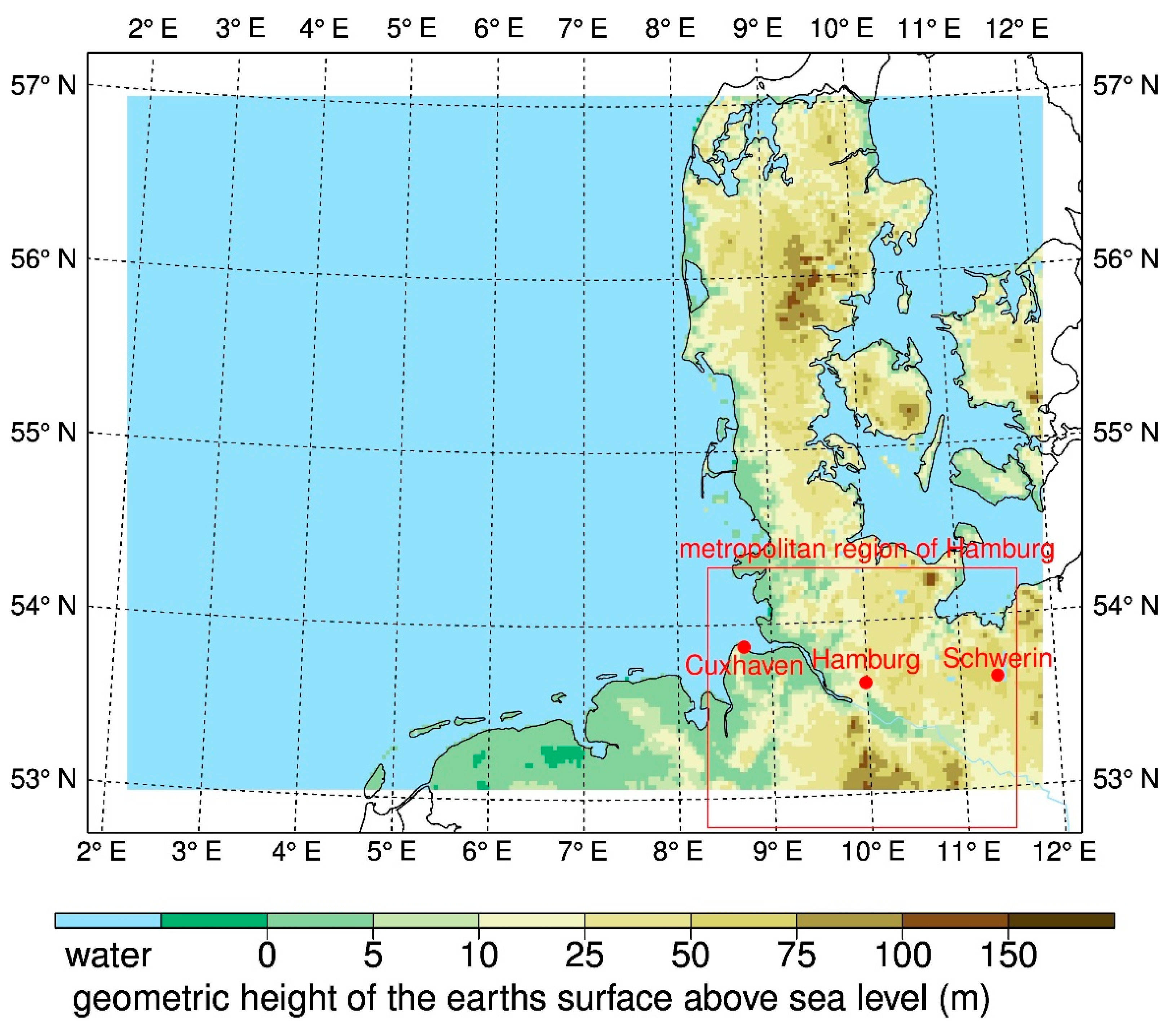
2.1. Model Configuration and Data

For the long-term evaluation, one consistent and uninterrupted simulation is analyzed [19]. The model domain covers the German Bight and the western part of the Baltic Sea with a spatial grid distance of 0.025° (about 2.8 km), 250 × 180 grid points, 40 vertical layers, a rotated pole at 8.82° E and 54.45° N, and a time step of 25 s. The lateral sponge zone has a width of 12 grid points, so we analyzed 226 × 156 grid points in this study. For this hindcast simulation the non-hydrostatic limited-area atmospheric model COSMO-CLM (version 5.0) [20,21] (CCLM), which is the climate version of the regional weather prediction model COSMO of the German weather service (DWD), is employed. In the following, this high-resolution long-term simulation will be referred to as GB0028. The simulation was run from January 1948 to August 2015. This is exactly the time period of coastDat II, which was used as forcing data. The coastDat II data set is an atmospheric reanalysis for Europe for the last 67 years, from January 1948 to August 2015 [22,23]. For the coastDat II reanalysis, NCEP/NCAR global reanalysis with a grid distance of 1.875° [24] was dynamically downscaled using the version 4.8 of the same, albeit hydrostatic regional CCLM model to a grid distance of 0.22 degrees (~24 km).
A variety of physical processes are taken into account by parameterization schemes in the CCLM model [25,26]. The most important and those with the most computing time are radiation, clouds, precipitation, turbulent fluxes schemes, and the soil model. The GB0028 simulation uses a grid point distance of 2.8 km and can thus simulate precipitating deep convection explicitly [11]. Therefore, the simulation only uses the shallow convection scheme. The shallow convection scheme is a simplified Tiedtke scheme [27]. For wind gusts, the standard parameterization of the DWD is used for this study. The wind gusts were derived from the wind speed in the lowest model layer and the friction velocity, which is parameterized after [28,29]. This parametrization is based on a two-component approach that contains turbulent and convective gusts. The spectral nudging (SN) technique described by [30] was applied for the coastDat II simulation to keep large weather systems (larger than about 1200 km) close to the large-scale atmospheric conditions simulated by the forcing reanalysis. Test simulations, which are referred to the 2.8 km simulation, with and without SN showed no significant differences and therefore lead to the conclusion that spectral nudging is not necessary for high-resolution simulation. This is presumably a consequence of the relatively small model domain, as spacious weather patterns which deviate from observed large weather systems have no time to develop inside this domain [31]. The data set was validated regarding added value of this high resolution of 2.8 km compared to a simulation with 24 km grid distance and observations for ten storm events [13]. It was shown that the simulation can reproduce storm events realistically and the added value of the convection-permitting resolution is mainly in synoptic comparisons of single storm cases. E.g., the frontal convective precipitation or the post-frontal subsidence can be simulated for storm Christian. For that reason, it can be assumed that a realistic representation of the atmospheric state is given.

2.2. Methods

For the analysis of GB0028 (see Chapter 3.3), 67 complete years of homogeneous meteorological data are available for the evaluation of long-term trends. This is one of the first of such long-term climate model simulations at a very high resolution of 2.8 km. Annual mean values (annual sums for precipitation) and 99th percentiles were calculated. Linear trends of the considered variables were calculated through linear regression, using the least squares method. For the evaluation of temporal tendencies, the annual and extreme trend indices were tested with the non-parametric Mann-Kendall test [32,33]. The tests are carried out at the nominal 5% level of significance. Additionally, the trend over the area-averaged values was calculated to evaluate the interannual variability and significance of the trends. All trends were calculated for the time period 1948–2014. For parameters that are of great importance for the human well-being, locations with special differences due to the spatial location were selected. In these locations, single grid points in Hamburg, Schwerin and over the North Sea were selected to compare the differing trends over the cities and the open ocean. Some trends of extreme events differed between land and sea areas.
To estimate the influence of coastDat II as a forcing for GB0028, we compare GB0028 with coastDat II, as well as with observations and additional data sets used in the web tool norddeutscher-klimamonitor.de [6] (see Chapter 3.1). The comparison is focused on the metropolitan region of Hamburg. To locate long-term changes, we compare the two time slices 1986–2015 and 1961–1990 (note that we used 1986–2014 in GB0028 and coastDat II, because September to December 2015 is missing). We used the period 1961–1990 because this is the commonly used normal period. The WMO defined the period from 1961–1990 as the international climatological reference period. For comparison, we have chosen the latest 30-year period of the simulation. For the calculation of the long-term changes, the difference of the mean of the two time slices was used. Besides coastDat II, there are five other data sets included in the web tool norddeutscher-klimamonitor.de [6]. These are (1) the re-analyzed coastDat I [34], (2) the interpolated global climate data set of the Climate Research Unit CRU TS 3.23 [35], (3) the interpolated temperature data set of the German weather service [36], (4) the interpolated climate data set for Europe from the EU-FP6 Project ENSEMBLES EOBS 14 based on daily observations [37] and (5) an interpolated global data set of the Department of Geography at the University of Delaware based on monthly observations [38].
For comparisons of the model simulation with station measurements at Cuxhaven, Hamburg, and Schwerin, a distance-weighted average of the four nearest neighbor grid point values was used for each model value, which means that not only the value of the grid box, which includes a certain station, is used, but also the surrounding grid boxes are considered. To compare the GB0028 data set with other gridded data set such as coastDat II, the data set was remapped to the GB0028 grid using the nearest neighbor approach. In this way, we kept the structure of the coarser grid, but still the same grid as the GB0028 data set.

3. Results

3.1. Time Slice Comparison of GB0028 with other Data Sets

According to long-term changes in the 2 m temperature as well as in precipitation sum, GB0028 is similar to the coastDat II forcing. This shows the comparison of GB0028 and coastDat II with the other data sets of the norddeutscher-klimamonitor.de mentioned in Chapter 2.3 and the station observation at Cuxhaven, Hamburg, and Schwerin (see Figure 1). These stations were chosen because they were the longest undisturbed time series within the model domain. The similarity in the long-term evaluation is due to the fact coastDat II was used as forcing data for GB0028. The advantage of the higher resolution is evident in the small-scale synoptic comparison of single weather situations [13]. From all data sets, coastDat II shows the lowest warming (2 m temperature increase of 0.6 °C) occurring for the area mean in the metropolitan region of Hamburg (Figure 1) between the two time intervals 1986–2015 and 1961–1990 (Table 1). Other data sets show a warming of about 0.8–0.9 °C (EOBS 14.0, CRU, and DWD NKDZ). The 2 m temperature increase of GB0028 (0.66 °C) is close to the coastDat II forcing. Also, in comparison to the station observations Cuxhaven (+0.9 °C), Hamburg (1 °C) and Schwerin (0.9 °C), coastDat II and GB0028 are both systematically cooler with values between 0.6 °C and 0.7 °C. According to long-term changes in precipitation, GB0028 is also similar to the coastDat II forcing. Both coastDat II and GB0028 show a decrease in the annual precipitation sum in the metropolitan region of Hamburg, whereas all other data sets and the station observations at Cuxhaven, Hamburg, and Schwerin (see www.nordeutscher-klimamonitor.de, [7]) show an increase in annual precipitation sum (Table 1).

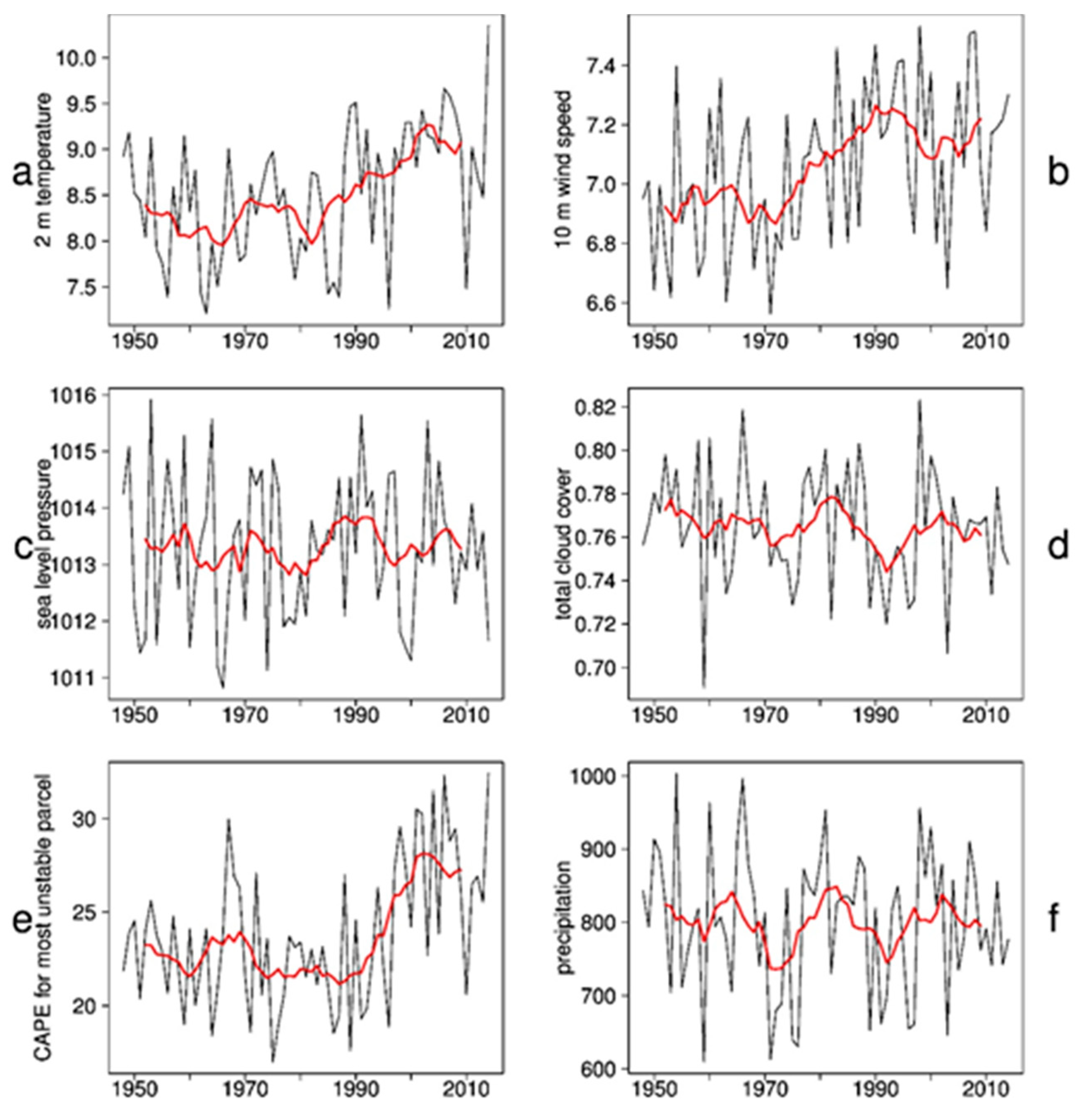
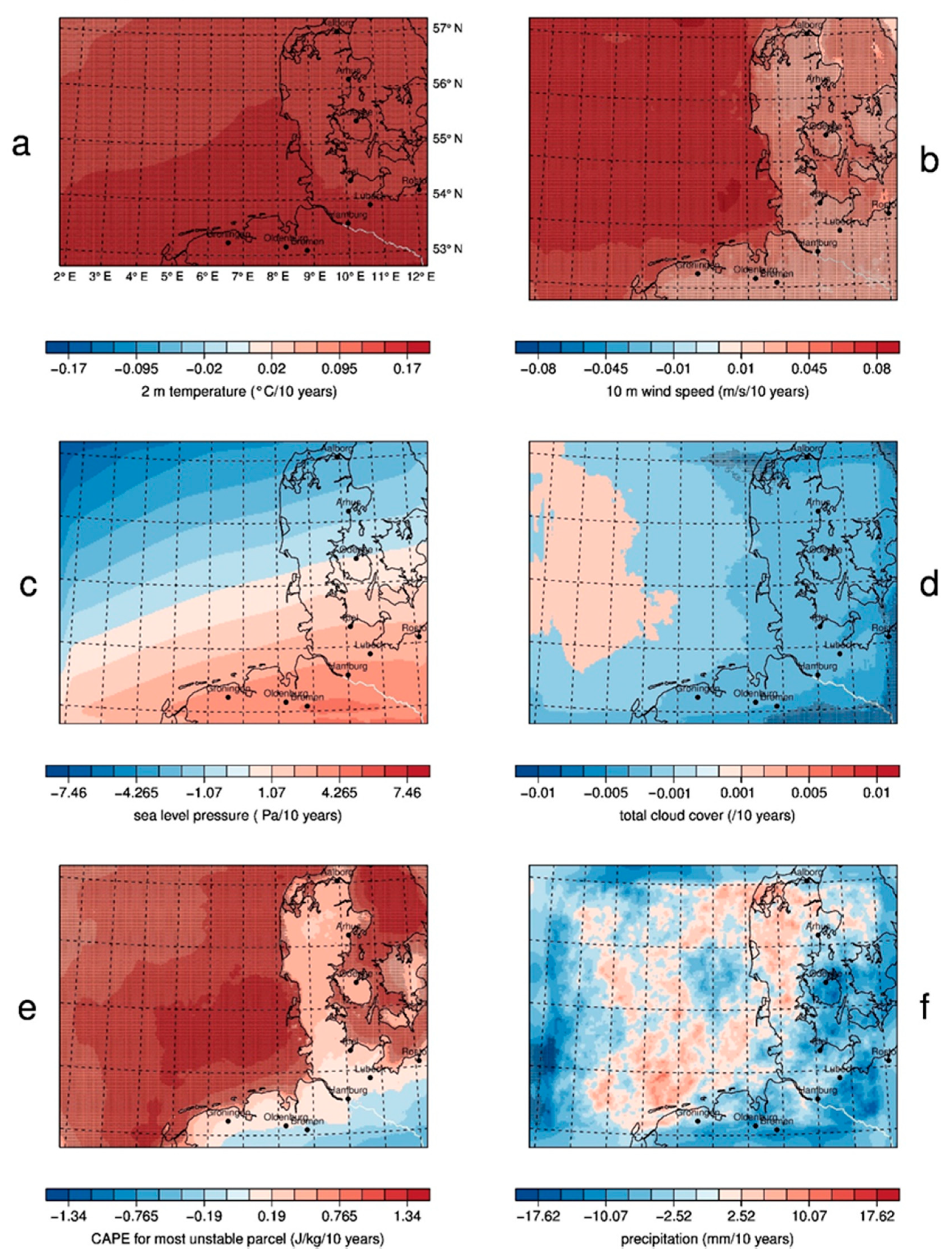
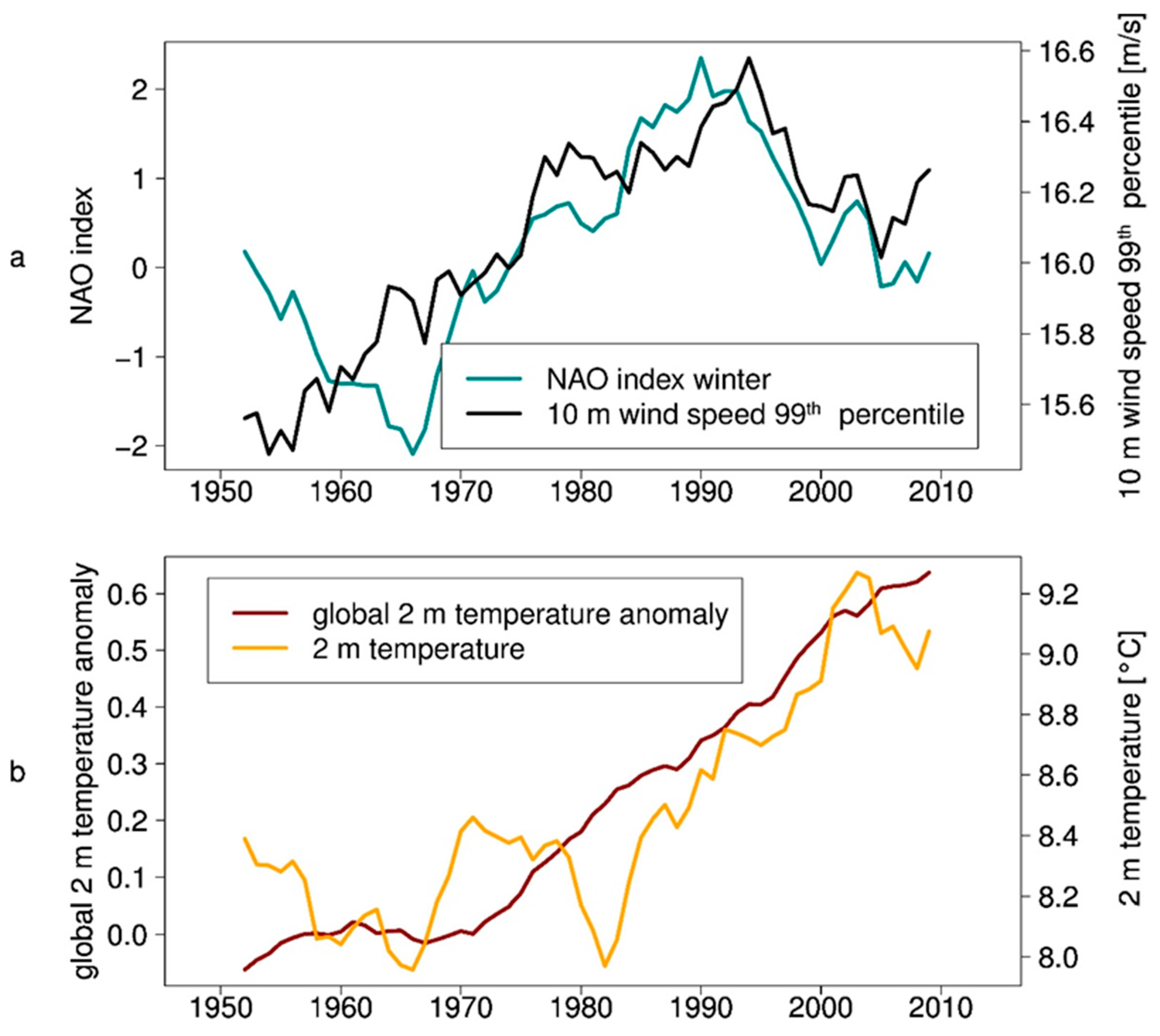
3.2. Trend Analysis of GB0028 over Northern Germany 1948–2014
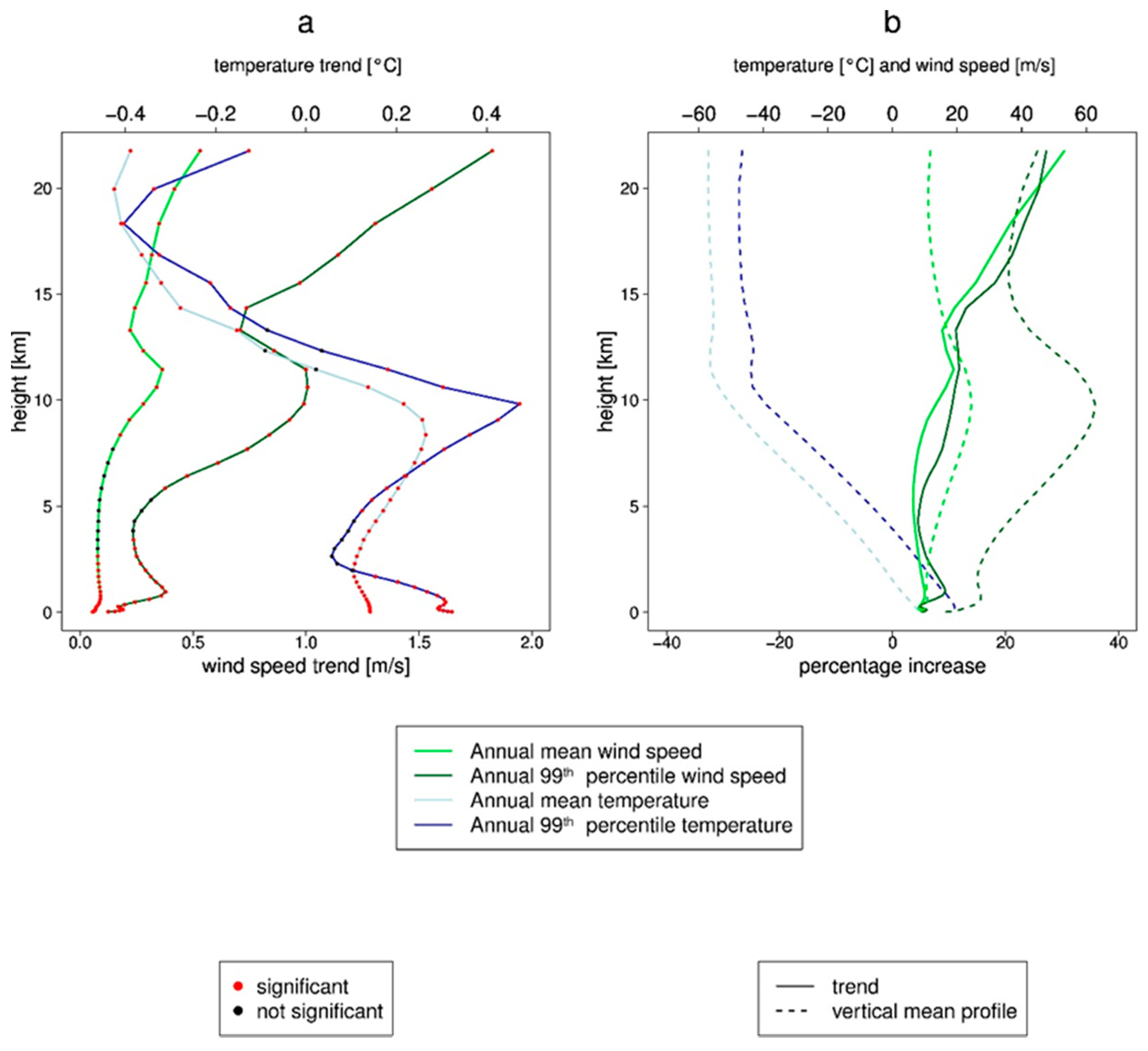
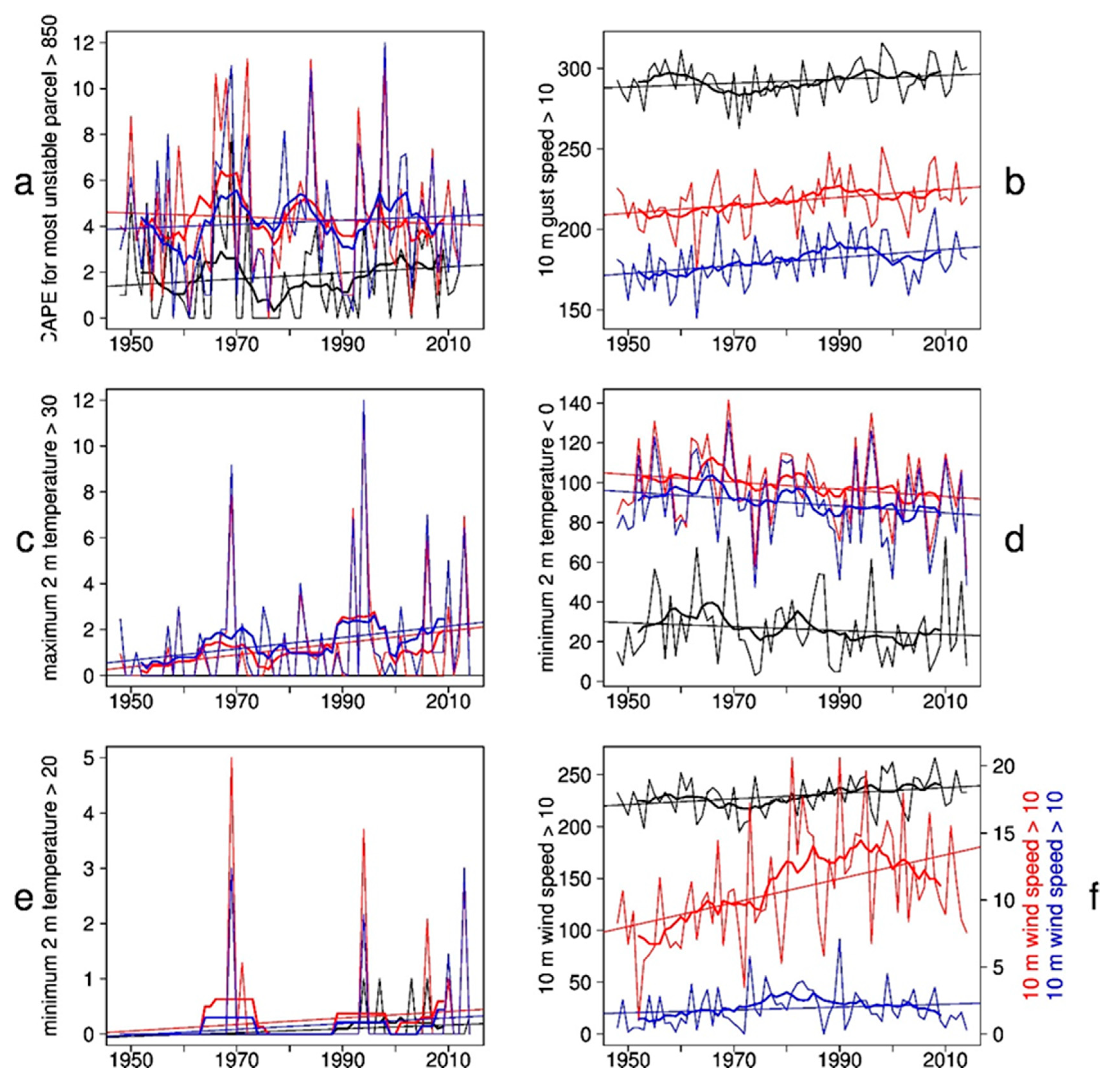
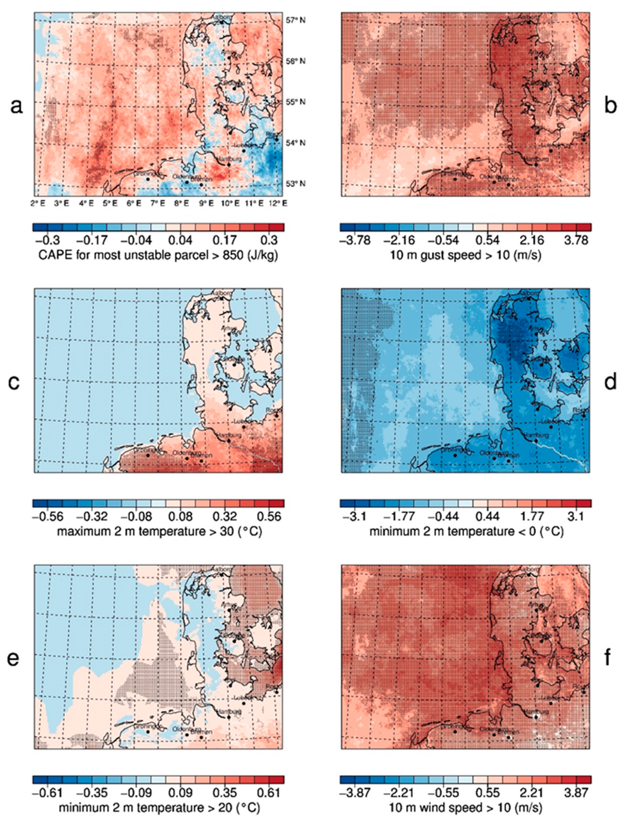
In this section, a long-term trend analysis of GB0028 is conducted for different variables. The section is divided into two parts. In the first part, annual mean values and total values for precipitation are presented. The second part contains extreme events with percentile calculations and maximum/minimum values.

3.2.1. Annual Means

The time series of the area-average of the annual values of a set of variables between 1948 and 2014 (Figure 2) reveal the interannual variability. Figure 3 shows decadal trends. Decadal trends between 1948 and 2014 of the annual values are presented. Grid points are marked with small black dots, if the trend signal of a grid point is significant according to the Mann-Kendall-test at the nominal 5% level. High variability in Figure 2 may show the reasons for the lack of significance.
The trends of the 2 m temperature (Figure 2 and Figure 3a) and 10 m wind speed (Figure 2b and Figure 3b) show the strongest signals with the highest significance for the entire model domain. Both show a clearly positive signal. The 2 m temperature trend has a weak gradient from north to south. This might be due to coastDat II showing a similar feature in the 2 m temperature trend, whereas other data sets do not [7]. The highest trend, with a 0.17 °C decadal increase of the annual mean temperature, can be found in this simulation at the southern edge of the model domain, in Northern Germany. The weakest trend with 0.12 °C per decade, occurs in Northern Denmark, at the Northern edge of the model domain. The trend values are relatively small for the period 1948–2014. This might be correlated with a slight cooling from the 1950s to the 1980s (see time series), which could be caused by increased aerosol concentrations [39]. The trend from the 1980s until present time is much higher. The interannual variability has a maximum of 2 °C, which means that the trend is significant. The 10 m wind speed also shows a positive trend for the entire model domain with a clear land-sea-separation. There are decadal trends of 0.08 m/s in the annual mean wind speed over the North Sea, where the highest absolute wind speeds occur. The further inland, the weaker the trend, but it remains positive with minimum values of 0.005 m/s. The patterns of the roughness length are visible in the trend, such that local effects of cities can be seen. In cities, where the absolute wind speed is reduced because of the high roughness length, the weakest trends are also visible, compared with the trends of absolute wind speeds in surrounding areas. The positive trends mainly result from increasing mean wind speeds in the 1980s and 1990s, where a phase of high storm activity took place [40,41]. After that phase, a decrease in storminess can be observed until it increases again in the beginning of the 2010s.
The variability of simulated wind speed and storminess generally follows the NAO index (Hurrell Station-Based DJFM NAO Index, Figure 4a), which shows large multi-decadal variability, but no long-term trend. On the contrary, the simulated 2 m temperature resembles the increasing global 2 m temperature (Global Land and Ocean Temperature Anomalies of NOAA) trend due to global warming (Figure 4b). Many studies [16,17,18,42] use the NAO index for analyzing changes in wind speed and temperature. However, the 10 m wind speed 99th percentile time series shows larger similarity with the NAO index (Figure 4a) than with the increasing near-surface temperature trend of recent decades (Figure 4b). The time correlation between the NAO index and the 99th percentile of 10 m wind speed is 0.76 for the 10 years running mean and 0.32 for annual values. Both curves in Figure 4a have a high correlation especially since the 1970s, which confirms the findings of [42], who report an increasing correlation of storms and the NAO index for more recent decades. The variability is very high and as [40,41] showed for geostrophic wind speed over the North Atlantic, there is no long-term (longer than the 67 years analyzed in this study) trend in wind speed and storminess. The correlation between the wind percentiles and the global temperature anomaly is low (0.2), which confirms that there is not a strong link between these variables. The 2 m temperature has a correlation of 0.87 with the global mean temperature anomaly (Figure 4b), which means that the temporal evolvement of the temperature in Northern Germany is quite similar to the global mean temperature. However, the variability of the rising temperature in Northern Germany is higher than the global temperature variability.
The interannual variability in the sea level pressure (Figure 2c and Figure 3c) and total cloud cover (Figure 2d and Figure 3d) are both very high which means that there is no clear and significant trend, and there are no clear decadal phases. Regarding sea level pressure, a strong north-south gradient is visible with negative values in the north and positive values in the south, which could point to a northward shift of low-pressure systems. This broadly agrees with [45] or [46]. In reanalysis data such a northward shift was shown by e.g., [47] for NCEP and [48] for ERA40. However, the trend values vary between +5 and −7 Pa per decade and the missing significance renders the assumption very weak.
The CAPE is defined as the amount of energy, which an air parcel achieves if it is lifted vertically into the atmosphere. It is an indicator for the instability of the atmosphere and therefore used for thunderstorm prediction [49]. The CAPE for most unstable particles (MUCAPE) is the highest possible CAPE and not surface-based. Its value results from rising the most unstable air package regardless of its height. High MUCAPE values larger than about 800 J/kg imply a high potential for thunderstorms [50]. If the MUCAPE values are higher, there is more energy “in the air” and thunderstorms become more likely. The time series of the annual MUCAPE means (Figure 2e) shows that the positive trend over the sea (Figure 3e) originates from the last two decades of the analyzed time period. The MUCAPE mainly increased significantly over sea areas, where the MUCAPE is normally relatively low and thunderstorms are rare because of non-existent orography. As CAPE depends on virtual temperature, both MUCAPE and near-surface temperature show some similarity, in their temporal variability (Figure 2a,e) and in their spatial trends (Figure 3a,e). Both time series show an increase during recent decades; however, for MUCAPE the increase is steeper, starting about 1990. The spatial trends (Figure 3a,e) both show an increase from the northwest towards the coasts over the ocean, but for temperature this pattern continues over land, while for MUCAPE the highest values over land are close to the coasts and they decrease further inland. Close to the coasts, orography is flat and low MUCAPE values prevail, but moisture values are larger than further inland. The spatial trend pattern of precipitation shows decreasing trends over land away from the coast, which may also influence moisture in these regions.
The interannual variability in the precipitation amount (Figure 2f and Figure 3f) is quite high and the model mean precipitation amount varies between 600 and 1000 mm per year. Therefore, the trend is not significant for the whole model domain. The strong negative values at the boundaries must be ignored. The boundary effect of the relaxation zone possibly extends further into the model domain than the sponge zone for precipitation.
Looking at the vertical trend of temperature and wind speed (Figure 5a) reveals a noticeable dependency of both trends on height. The positive trend of the wind speed increases with height. This increase is significant at all heights except for those between 4 and 8 km. The temperature trend decreases with increasing height and becomes negative at the top of the atmosphere at a height of about 13 km and above. This is also the case for the mean temperature and for the extreme temperature trend (99th percentile). However, the 99th percentile of the wind speed shows a different behavior. The extreme wind speeds show a much more intense increase of the trend with increasing height. A trend of 2 m/s per decade is present at the top of the troposphere. The absolute values in this height are certainly higher than in the boundary layer. Furthermore, the relative trend (Figure 5b) also shows that the trend increases with height for the mean and extreme wind speed at the same extent. However, it is not clear whether the trends are caused by the regional climate model, or whether the forcing data (especially at the top of the model domain, where the Rayleigh damping takes place) affect the modeled variables and possibly induce artificial trends.

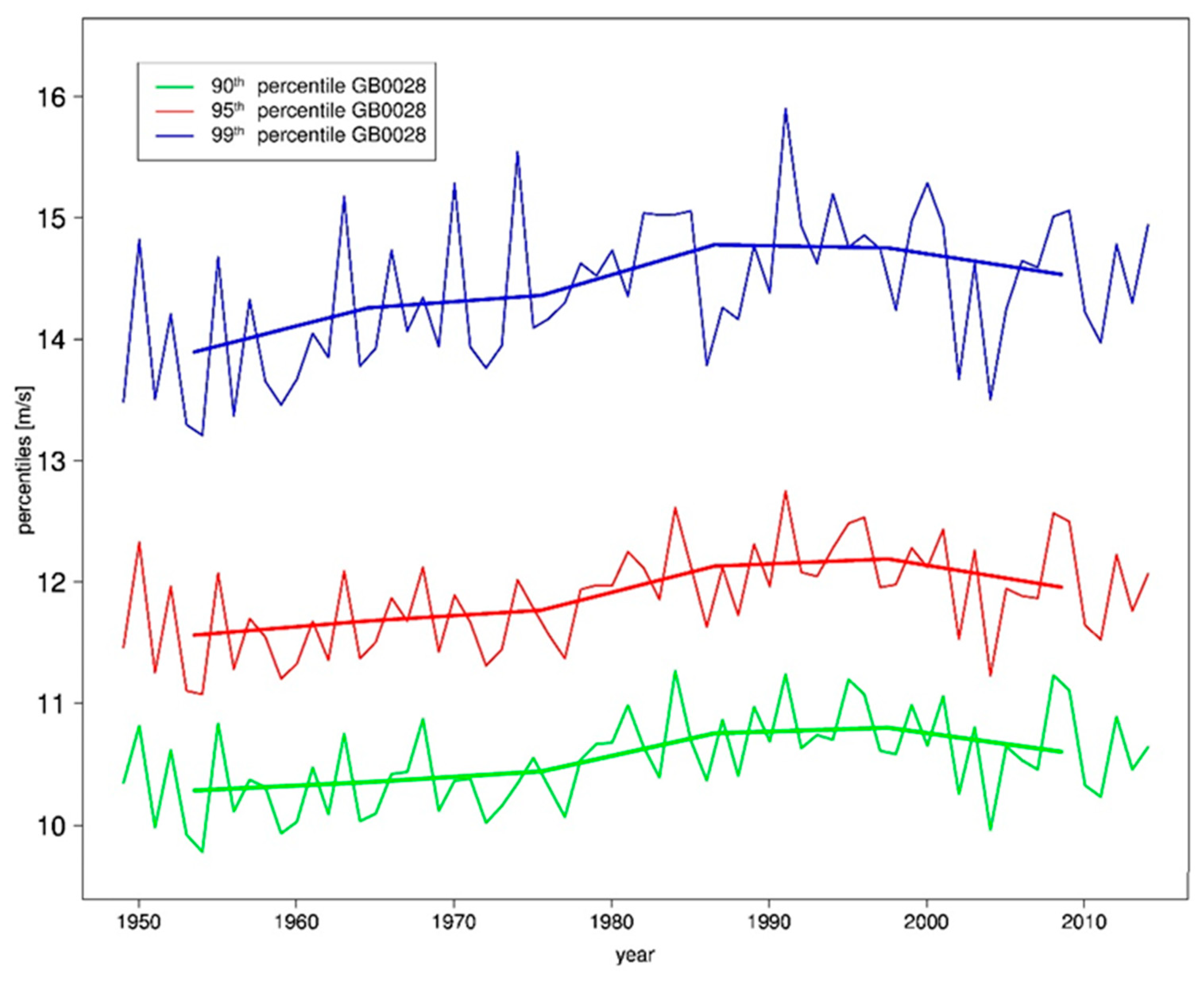
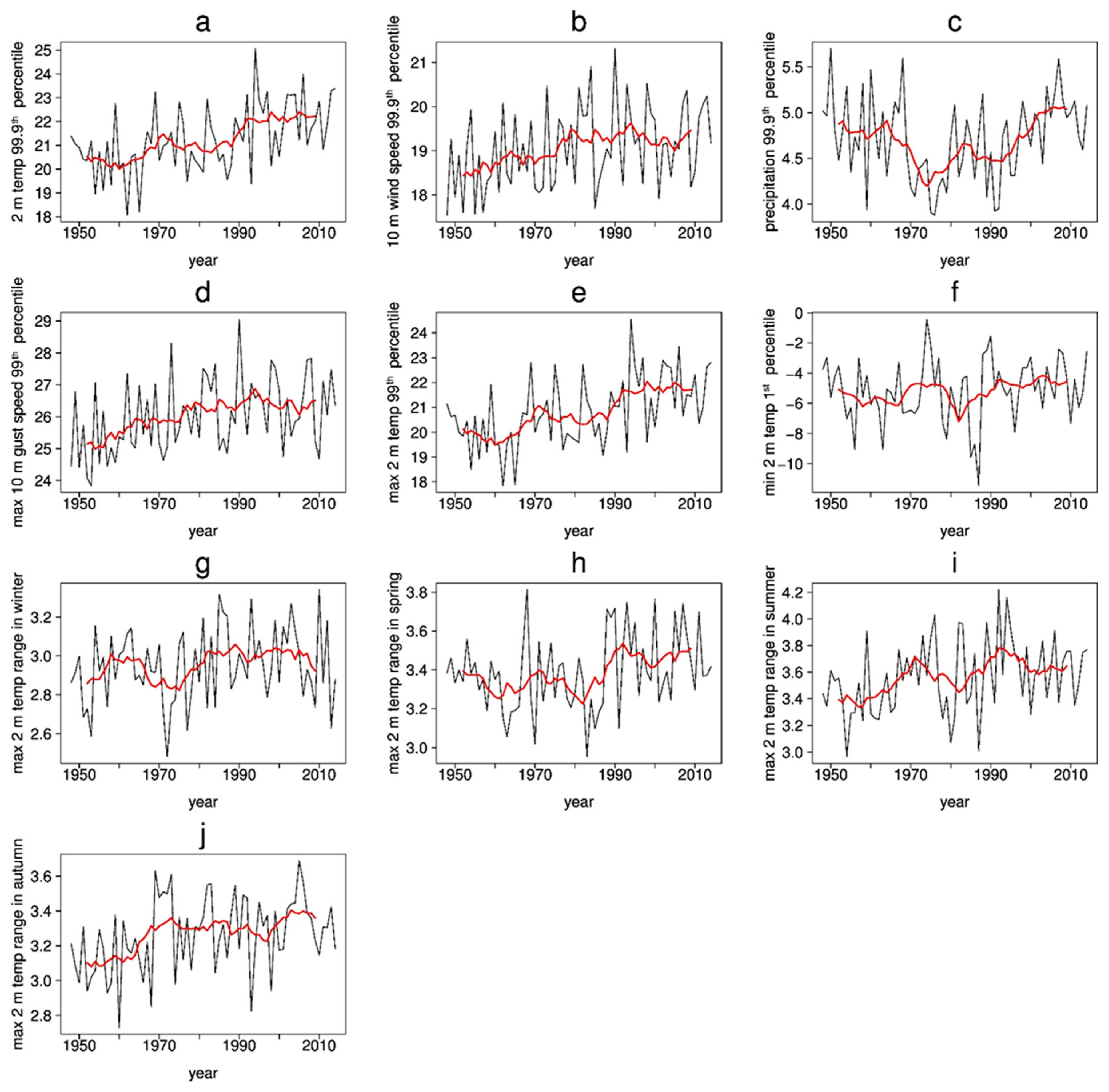
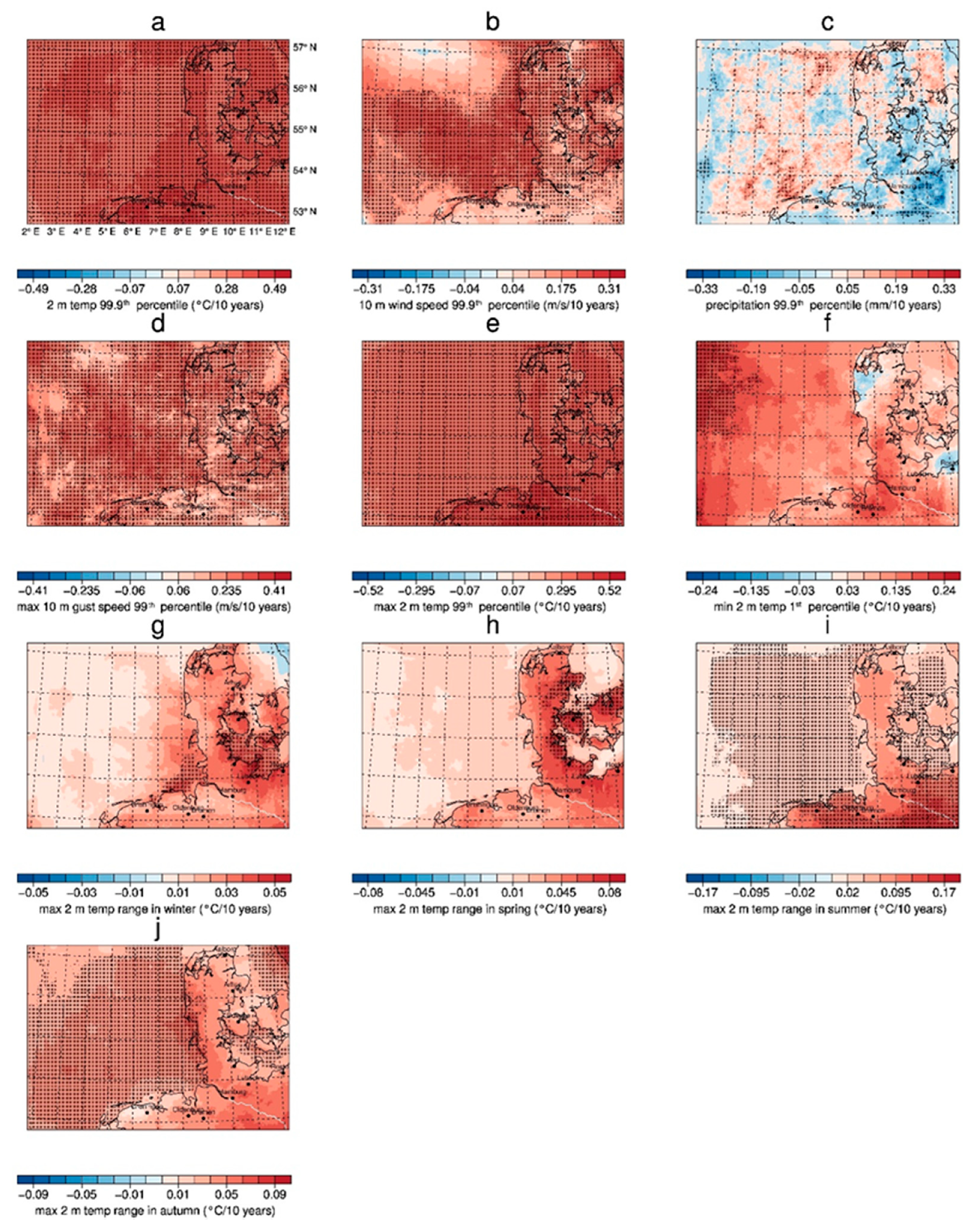
3.2.2. Extreme Events

The occurrence of extreme events indicated by percentiles and the frequency of events beyond a certain threshold are also noteworthy, in addition to the annual mean values. The question arises: Do extreme events have local effects that occur only in small and confined areas?
To get a general overview of the development of storminess in the last seven decades, different percentiles of the 10 m wind speed are evaluated (Figure 6). One can see a similar behavior of the 90th, 95th, and 99th percentile curves. There was a stormy phase in the 1990s with high percentile values and a decrease of the extreme wind speeds afterwards. This result is similar to the result in Chapter 3.2.1 on the mean 10 m wind speed trend.
For the evaluation of extreme events, it is suitable to evaluate annual percentiles of the considered variables to compare all years over the entire period of GB0028 devoid of intra-annual cycles. The 99.9th percentiles are calculated for hourly data, i.e., the values of only nine hours per year are more extreme than the shown value. The 99th percentiles are calculated for daily data, which means that extreme values can only be found on three days a year. The analysis of the variability of a set of meteorological variables is presented in Figure 7 and Figure 8. Figure 7 shows associated pattern mean time series, corresponding to Chapter 3.2.1 for the annual means; Figure 8 shows the spatial pattern of the trends.
The 99.9th domain mean percentile of the 2 m temperature (Figure 7a and Figure 8a) increases from about 20 °C in the 1950s to about 23 °C in the 2010s, which is dominated by the relatively cool temperature over the North Sea. It shows, similar to the annual mean, an increase of the extreme values of about 0.5 °C per decade, which is statistically significant for the whole model domain. The 10 m wind speed behaves similarly (Figure 7b and Figure 8b) with a significant positive signal especially over the German Bight region and over the North Sea, where the highest wind speeds already occur. However, the interannual variability is very high with an intense phase of storminess in the 1990s just like in the annual mean. The extreme precipitation interannual variability (Figure 7c and Figure 8c) is very high with quite similar and none significant trends. The time series of extreme precipitation show a less extreme period in the 1970s and 1980s and more extreme precipitation before that and after that. The 99th percentile of the daily maximum 10 m gust speed (Figure 7d and Figure 8d) shows a significant positive trend of about 0.4 m/s per decade in the entire model domain, where the low-passed time series is very similar to the time series obtained for the annual 99.9th percentiles of wind speed. With 67 years, quite a short period of time (regarding storminess) was examined, in which storminess generally increased even though there was a decrease in the 2000s. The trend for the entire 1948 to 2014 period is still positive. The values have the same magnitude over sea as over land. There are some local structures in the trend, but no clear region, where the gust trend is favored. The stormy 1990s in the time series are not as intensive for the gusts as for the wind speed without gusts. There is a continuous increase of the 99th percentile, which represents the minimum of the 3–4 windiest days (including gusts) per year.
A further important question for the human well-being is whether the hottest (Figure 7e and Figure 8e) and coolest (Figure 7f and Figure 8f) days have changed. The 99th percentiles of the daily maximum 2 m temperature show a strong significant increase of temperature with values of 0.5 °C per decade over the Northern German land areas. The interannual variability is low, so the trend is quite clear. The interannual variability of the first percentile of the daily minimum 2 m temperature is higher than for the hottest days, which causes the temperature signal not to be significant. The trend is about three times smaller than the trend of the hottest days and not clear due to the high variability. However, it shows some hot spots at the North Sea Coast and in the regions around Hamburg and Bremen.
The trend of the diurnal temperature range (DTR) is analyzed for seasonal time scales to show the different behavior of the seasons. Shown is the trend of the highest annual seasonal DTR (Tmax–Tmin), which is an important index of climate change [51] and is also relevant for local climatic studies in limited-area domains [52] (Figure 7g–j and Figure 8g–j). In the winter and spring seasons there is a strong but not significant increase in the DTR over land areas. This is caused by the increasing Tmax. The DTR is not as strong over sea as over land, because of the temperature-dampening effect of the sea, which prevents a cooling of the air temperature at night. In the summer and autumn seasons, the positive trend is mainly significant and is highest as the extreme temperatures increase significantly (Figure 8e).
Looking at the number of days with threshold exceedances reduces inherent autocorrelation and prevents from counting consecutive time steps multiple times, as opposed to the 99.9th percentile of hourly data in the previous section. Figure 9 shows time series of the number of days of a set of climate indices for three different locations and Figure 10 shows the trend. The chosen locations are location in the middle of the North Sea, a grid point in the center of Hamburg, and a grid point in Schwerin, a small city further inland about 100 km east of Hamburg, in the vicinity of a large lake, and more influenced by continental weather patterns. MUCAPE values larger than 850 J/kg imply a strong potential for thunderstorms. The total number of these days is normally lower than 10 for all three locations and therefore it is difficult to get a significant trend (Figure 9a). Therefore, the trend (Figure 10a) is not clear. The time series for Hamburg shows a higher number of high MUCAPE days than in the one of Schwerin during the last 20 years. There is a large discrepancy in the number of days with 10 m wind gusts higher than 10 m/s between the North Sea and Hamburg (Figure 9b). Over the North Sea there are gusts with intensities over 10 m/s almost every day, while for Hamburg such gusts happen every second day only. Although the number over the North Sea is high, the trend is not significant everywhere (Figure 10b) as the variability is high. In Hamburg, the number of days is even lower than in Schwerin. For hot days (maximum 2 m temperature higher than 30 °C), only a trend over the Northern German mainland is visible as there are no temperatures above 30 °C in Denmark and over the sea (Figure 10c) due to a stronger warming of landmasses in summer times. The trend is clearly positive with an increase of 0.5 hot days per decade and is partly significant because the variability is low. In the first decade of the analyzed period, there is a maximum of two hot days in Hamburg and Schwerin. In more recent periods, hot days often occur more than 5 times per year (Figure 9c). The number of frost days (lowest 2 m temperature below 0 °C) decreases in the entire model domain (Figure 10d). The magnitude of the trend is quite large with 3 frost days less per decade in Denmark, 2 days less in Northern Germany and 1 day less over the ocean. Considering the number of 20–30 frost days over the ocean and around 90 days over land, the trend is quite robust (Figure 9d).
Tropical nights (lowest 2 m temperature higher than 20 °C) do not occur often in the model domain, but are very important for human well-being. Over the North Sea and the adjacent land area, the number of tropical nights is increasing. From the 1990s onwards, they occur every year at least once (Figure 9e). Over the Baltic Sea the trend is stronger and significant (Figure 10e). Here, they occur more often due to the warmer sea surface temperature of the Baltic Sea compared to the North Sea. In addition, lower wind speeds and related reduced cooling over the Baltic Sea contribute to the increase. Days with 10 m wind speeds greater than 10 m/s occur less often than gust speeds exceeding 10 m/s. In Hamburg, there was only one day in the analyzed period of 67 years (in the year 1990) with a wind speed greater than 10 m/s. This is a consequence of the high roughness length in Hamburg. Therefore, no trend evaluation for Hamburg is possible (Figure 9f). For all other regions, there is similar behavior as found for the annual mean wind speed and the 99.9th wind speed percentiles before (Figure 10f).

4. Summary and Discussion

The question of how the long-term variability in a convection-permitting simulation of the most important meteorological variables was appears to have been answered. For this purpose, a very high-resolution simulation was carried out with the regional climate model COSMO-CLM (CCLM) at a grid distance of 2.8 km for the region of the German Bight and Northern Germany from 1948–2014. Climatologies of annual mean values and extreme events of variables were computed for this region.
The long-term variability analysis revealed that GB0028 provides the most distinct and significant trends for 2 m temperature and CAPE. These variables showed an increase in the last seven decades in all the following cases: There is an increase for annual mean values as well as for extreme events like 99th percentiles, hot days, or number of days with high potential for thunderstorms. The increase of the annual mean 2 m temperature is about 0.17 °C per decade in the model domain. This is below the trends documented for the metropolitan region of Hamburg by [4]. Based on the data sets coastDat I and II [23,34] the trends of the annual mean temperature from 1951–2010 is about 0.2 °C per decade in the metropolitan region of Hamburg and in Northern Germany [4]. Moreover, observations of 12 weather stations in Northern Germany show higher decadal trends between 0.2 °C per decade at Brocken, up to 0.28 °C per decade in Rostock Warnemünde [4]. Wind speeds showed low variability until the 1980s, confirming the findings of [53], who found a stationary annual distribution of geostrophic wind speeds over the German Bight between 1880 and 1990. Thereafter, there was an intense phase of storm activity during the 1990s resulting in an overall increasing wind. Since the end of the 1990s, the trend of the wind speed has been decreasing. Other studies show an increase of mean wind speed over the southern North- and Baltic Sea since 1960 [54] and an increase of annual mean wind speed and storm intensity over the metropolitan region of Hamburg and Northern Germany [4]. According to the storm frequency, Feser et al. [55] documented an agreement among several studies according to an increased storm frequency between 1960 to 1995 over the North Atlantic (55–60°) and a subsequent decrease afterwards.
No clear and no significant trend is detectable for the annual sum of precipitation and for extreme precipitation in the new very high-resolution CCLM run. Increasing convective inhibition (CIN) might suppress the increase in CAPE and therefore inhibit the increase in extreme precipitation. Looking at Europe, there tends to be no change in the intensity with decadal variability present, which was confirmed by [56]. However, [4] documented disagreement among different studies according to annual precipitation amount. The cloud cover change in the past seven decades is not significantly due to high variability. The trend of CAPE for the most unstable parcel and the number of days with potential thunderstorms slightly increased. As CAPE depends on virtual temperature, both MUCAPE and near-surface temperature show some similarity, in their temporal variability, which shows an increase during the most recent decades, and in their spatial trends over the ocean. The number of frost days became less, and the coldest nights became warmer. The daily temperature range, which is an important index of climate change, increased mainly over land areas and mainly in the summertime.
The 2 m temperature trend as a large-scale variable did not show any notable spatial structures. In addition, the trends in CAPE for most unstable parcels did not show regional effects, for which the high resolution of 2.8 km is necessary. For wind speed, some local effects such as lower trends in the cities are visible as the absolute wind speed is lower over areas with increased (and increasing) surface roughness. In addition, many regional small-scale details in the precipitation trends are present. However, as they are not significant at all, such details can be considered to be randomly distributed with no significant impact on the trends of precipitation.
A long-term simulation with convection-permitting resolution covering larger areas would provide more valuable insights to our research and should be done as future work. It is unfortunately not feasible currently because of the enormous computing time needed at such high resolution.

Author Contributions

Conceptualization, B.S.; Data curation, B.S.; Formal analysis, B.S.; Investigation, B.S.; Methodology, B.S.; Visualization, B.S.; Writing—original draft, B.S.; Writing—review and editing, F.F. and I.M.

Funding

The work was supported through the Cluster of Excellence ‘CliSAP’ (EXC177), Universität Hamburg, funded through the German Research Foundation (DFG).

Acknowledgments

The work was supported through the Cluster of Excellence ‘CliSAP’ (EXC177), Universität Hamburg, funded through the German Research Foundation (DFG). It is a contribution to the Helmholtz Climate Initiative REKLIM (Regional Climate Change), a joint research project of the Helmholtz Association of German research centers (HGF). The German Climate Computing Center (DKRZ) provided the computer hardware for the regional climate model simulations. We would like to thank Marc Buckley for proofreading this paper.

Conflicts of Interest

The authors declare no conflict of interest.

References

  1. IPCC. Climate Change 2013: The Physical Science Basis. Contribution of Working Group I to the Fifth Assessment Report of the Intergovernmental Panel on Climate Change; Cambridge University Press: Cambridge, UK; New York, NY, USA, 2013; p. 1535. [Google Scholar]
  2. Roshan, G.; Yousefi, R.; Fitchett, J.M. Long-term trends in tourism climate index scores for 40 stations across Iran: The role of climate change and influence on tourism sustainability. Int. J. Biometeorol. 2016, 60, 33–52. [Google Scholar] [CrossRef] [PubMed]
  3. Caloiero, T.; Coscarelli, R.; Ferrari, E.; Sirangelo, B. Trend analysis of monthly mean values and extreme indices of daily temperature in a region of southern Italy. Int. J. Climatol. 2017, 37, 284–297. [Google Scholar] [CrossRef]
  4. Meinke, I.; Rechid, D.; Tinz, B.; Maneke, M.; Lefebvre, C.; Isokeit, E. Klima der Region – Zustand, bisherige Entwicklung und mögliche Änderungen bis 2100. In Hamburger Klimabericht – Wissen über Klima, Klimawandel und Auswirkungen in Hamburg und Norddeutschland; Von Storch, H., Meinke, I., Claußen, M., Eds.; Springer: Berlin/Heidelberg, Gemany, 2018; pp. 15–36. [Google Scholar]
  5. Schefczyk, L.; Heinemann, G. Climate change impact on thunderstorms: Analysis of thunderstorm indices using high-resolution regional climate simulations. Meteorol. Z. 2017, 26, 409–419. [Google Scholar] [CrossRef]
  6. Meinke, I.; Maneke, M.; Riecke, W.; Tinz, B. Norddeutscher Klimamonitor–Klimazustand und Klimaentwicklung in Norddeutschland innerhalb der letzten 60 Jahre (1951–2010). Mitteilungen DMG 012014. 2014. Available online: https://www.hzg.de/imperia/md/content/klimabuero/norddeutscher_klimamonitor.pdf (accessed on 8 January 2018).
  7. Klimamonitor, Norddeutscher Klimamonitor. Available online: http://www.norddeutscher-klimamonitor.de/ (accessed on 21 January 2018).
  8. Quante, M.; Colijn, F. North Sea Region Climate Change Assessment. Available online: https://doi.org/10.1007/978-3-319-39745-0 (accessed on 23 January 2019).
  9. The BACC II Author Team. Second Assessment of Climate Change for the Baltic Sea Basin; Springer: Berlin, Germany, 2015. [Google Scholar]
  10. Von Storch, H.; Meinke, I.; Claussen, M. Hamburger Klimabericht–Wissen über Klima, Klimawandel und Auswirkungen in Hamburg und Norddeutschland. Available online: https://doi.org/10.1007/978-3-662-55379-4 (accessed on 23 January 2019).
  11. Prein, A.F.; Langhans, W.; Fosser, G.; Ferrone, A.; Ban, N.; Keller, K.G.M.; Tölle, M.; Gutjahr, O.; Feser, F.; Brisson, E.; et al. A review on regional convection-permitting climate modeling: Demonstrations, prospects, and challenges. Rev. Geophys. 2015, 52, 323–361. [Google Scholar] [CrossRef]
  12. Prein, A.F.; Gobiet, A.; Suklitsch, M.; Truhetz, H.; Awan, N.K.; Keuler, K.; Georgievski, G. Added value of convection permitting seasonal simulations. Clim. Dyn. 2013, 41, 2655–2677. [Google Scholar] [CrossRef] [Green Version]
  13. Schaaf, B.; Feser, F. Is there added value of convection-permitting regional climate model simulations for storms over the German Bight and Northern Germany? Meteorol. Hydrol. Water Manag. 2018. [Google Scholar] [CrossRef]
  14. Brisson, E.; van Weverberg, K.; Demuzere, M.; Devis, A.; Saeed, S.; Stengel, M.; van Lipzig, N.P.M. How well can a convection-permitting climate model reproduce decadal statistics of precipitation, temperature and cloud characteristics? Clim. Dyn. 2016, 47, 3043–3061. [Google Scholar] [CrossRef] [Green Version]
  15. Liu, C.; Ikeda, K.; Rasmussen, R.; Barlage, M.; Newman, A.J.; Prein, A.F.; Chen, F.; Chen, L.; Clark, M.; Dai, A.; et al. Continental-scale convection-permitting modeling of the current and future climate of North America. Clim. Dyn. 2017, 49, 71–95. [Google Scholar] [CrossRef]
  16. Dawson, A.G.; Hickey, K.; Holt, T.; Elliott, L.; Dawson, S.; Foster, I.D.L.; Wadhams, P.; Jonsdottir, I.; Wilkinson, J.; McKenna, J.; et al. Complex North Atlantic Oscillation (NAO) Index signal of historic North Atlantic storm-track changes. Holocene 2002, 12, 363–369. [Google Scholar] [CrossRef]
  17. Hurrell, J.W.; Deser, C. North Atlantic climate variability: The role of the North Atlantic Oscillation. Impact Clim. Var. Mar. Ecosyst. Comp. Approach 2010, 79, 231–244. [Google Scholar] [CrossRef]
  18. Iles, C.; Hegerl, G. Role of the North Atlantic Oscillation in decadal temperature trends. Environ. Res. Lett. 2017, 12, 114010. [Google Scholar] [CrossRef]
  19. Schaaf, B. CoastDat_COSMO-CLM German Bright 0028. Available online: https://doi.org/10.1594/WDCC/coastDat_COSMO-CLM_GB0028 (accessed on 23 January 2019).
  20. Steppeler, J.; Doms, G.; Schättler, U.; Bitzer, H.W.; Gassmann, A.; Damrath, U.; Gregoric, G. Meso-gamma scale forecasts using the nonhydrostatic model LM. Meteorol. Atmos. Phys. 2003, 82, 75–96. [Google Scholar] [CrossRef]
  21. Rockel, B.; Castro, C.L.; Pielke, R.A.; von Storch, H.; Leoncini, G. Dynamical downscaling: Assessment of model system dependent retained and added variability for two different regional climate models. J. Geophys. Res. 2008, 113, D21103. [Google Scholar] [CrossRef]
  22. Geyer, B.; Rockel, B. Coastdat-2 COSMO-CLM. 2013. Available online: http://cera-www.dkrz.de/WDCC/ui/Compact.jsp?acronym=coastDat-2_COSMO-CLM (accessed on 23 January 2019).
  23. Geyer, B. High-resolution atmospheric reconstruction for Europe 1948–2012: coastDat2. Earth Syst. Sci. Data 2014, 6, 147–164. [Google Scholar] [CrossRef]
  24. Kalnay, E.; Kanamitsu, M.; Kistler, R.; Collins, W.; Deaven, D.; Gandin, L.; Iredell, M.; Saha, S.; White, G.; Woollen, J.; et al. The NCEP/NCAR 40-year reanalysis project. Bull. Am. Meteorol. Soc. 1996, 77, 437–471. [Google Scholar] [CrossRef]
  25. Schulz, J.P.; Schaettler, U. Kurze Beschreibung des Lokal-Modells Europa COSMO-EU (LME) und seiner Datenbanken auf dem Datenserver des DWD. 2009. Deutscher Wetterdienst. Available online: http://www.dwd.de/bvbw/generator/Sites/DWDWWW/Content/Forschung/FE1/Veroeffentlichungen/Download/LME__DBbeschr__0901,templateId=raw,property=publicationFile.pdf/LME_DBbeschr_0901.pdf (accessed on 23 January 2019).
  26. Doms, G.; F¨orstner, J.; Heise, E.; Herzog, H.-J.; Mironov, D.; Raschendorfer, M.; Reinhardt, T.; Ritter, B.; Schrodin, R.; Schulz, J.-P.; et al. A Description of the Nonhydrostatic Regional COSMO Model. Part II: Physical Parameterization. Deutscher Wetterdienst. 2011. Available online: http://www.cosmo-model.org/content/model/documentation/core/cosmoPhysParamtr.pdf (accessed on 23 January 2019).
  27. Tiedtke, M. A Comprehensive Mass Flux Scheme for Cumulus Parameterization in Large-scale Models. Mon. Weather Rev. 1989, 117, 1779–1800. [Google Scholar] [CrossRef]
  28. Schulz, J.-P.; Heise, E. A new scheme for diagnosing near-surface convective gusts. COSMO Newsl. 2003, 3, 221–225. [Google Scholar]
  29. Schulz, J.-P. Revision of the turbulent gust diagnostic in the COSMO model. COSMO Newsl. 2008, 8, 17–22. [Google Scholar]
  30. Von Storch, H.; Langenberg, H.; Feser, F. A Spectral Nudging Technique for Dynamical Downscaling Purposes. Mon. Weather Rev. 2000, 128, 3664–3673. [Google Scholar] [CrossRef]
  31. Schaaf, B.; von Storch, H.; Feser, F. Does Spectral Nudging Have an Effect on Dynamical Downscaling Applied in Small Regional Model Domains? Mon. Weather Rev. 2017, 145, 4303–4311. [Google Scholar] [CrossRef] [Green Version]
  32. Mann, H.B. Nonparametric Tests against Trend. Econometrica 1945, 13, 245–259. [Google Scholar] [CrossRef]
  33. Kendall, M.G. Rank Correlation Methods. Available online: https://onlinelibrary.wiley.com/doi/abs/10.1111/j.2044-8317.1956.tb00172.x (accessed on 23 January 2019).
  34. Weisse, R.; von Storch, H.; Callies, U.; Chrastansky, A.; Feser, F.; Grabemann, I.; Günther, H.; Pluess, A.; Stoye, T.; Tellkamp, J.; et al. Regional Meteorological–Marine Reanalyses and Climate Change Projections. Bull. Am. Meteorol. Soc. 2009, 90, 849–860. [Google Scholar] [CrossRef]
  35. University of East Anglia Climatic Research Unit (CRU). CRU TS3.20, Climatic Research Unit (CRU) Time-Series (TS) Version 3.20 of High Resolution Gridded Data of Month-by-month Variation in Climate (Jan. 1901–Dec. 2011); NCAS British Atmospheric Data Centre: Leeds, UK, 2013. [Google Scholar]
  36. DWD Climate Data Center (CDC), Raster der Monatsmittel der Lufttemperatur (2m) für Deutschland, Version v1.0. Available online: http://ftp-cdc.dwd.de/pub/CDC/grids_germany/monthly/air_temperature_mean/ (accessed on 27 June 2018).
  37. Haylock, M.R.; Hofstra, N.; Klein Tank, A.M.G.; Klok, E.J.; Jones, P.D.; New, M. A European daily high-resolution gridded data set of surface temperature and precipitation for 1950–2006. J. Geophys. Res. Atmos. 2008, 113. [Google Scholar] [CrossRef]
  38. Willmott, C.J.; Matsuura, K. Terrestrial Air Temperature, Gridded Monthly Time Series (1950–2014) (V 4.01). 2015. Available online: http://climate.geog.udel.edu/~climate/html_pages/Global2014/README.GlobalTsT2014.html (accessed on 27 June 2018).
  39. Schultze, M.; Rockel, B. Direct and semi-direct effects of aerosol climatologies on long-term climate simulations over Europe. Clim. Dyn. 2017. [Google Scholar] [CrossRef]
  40. Alexandersson, H.; Tuomenvirta, H.; Schmith, T.; Iden, K. Trends of storms in NW Europe derived from an updated pressure data set. Clim. Res. 2000, 14, 71–73. [Google Scholar] [CrossRef] [Green Version]
  41. Krueger, O.; Feser, F.; Weisse, R. Northeast Atlantic Storm Activity and Its Uncertainty from the Late Nineteenth to the Twenty-First Century. J. Clim. 2019, 32, 1919–1931. [Google Scholar] [CrossRef]
  42. Matulla, C.; Schöner, W.; Alexandersson, H.; von Storch, H.; Wang, X.L. European storminess: Late nineteenth century to present. Clim. Dyn. 2008, 31, 125–130. [Google Scholar] [CrossRef]
  43. Hurrell Station-Based DJFM NAO Index. Available online: https://climatedataguide.ucar.edu/sites/default/files/nao_station_djfm.txt (accessed on 27 June 2018).
  44. Global Land and Ocean Temperature Anomalies. Available online: https://www.ncdc.noaa.gov/cag/global/time-series/globe/land_ocean/ytd/12/1880-2018.csv (accessed on 27 June 2018).
  45. Barcikowska, M.; Feser, F.; Zhang, W.; Mei, W. Changes in intense tropical cyclone activity for the western North Pacific during the last decades derived from a regional climate model simulation. Clim. Dyn. 2017, 49, 2931–2949. [Google Scholar] [CrossRef] [Green Version]
  46. Barcikowska, M.J.; Weaver, S.J.; Feser, F.; Russo, S.; Schenk, F.; Stone, D.A.; Zahn, M. Euro-Atlantic winter storminess and precipitation extremes under 1.5 °C versus 2 °C warming scenarios. Earth Syst. Dyn. Discuss. 2018, 9. [Google Scholar] [CrossRef]
  47. McCabe, G.J.; Clark, M.P.; Serreze, M.C. Trends in Northern Hemisphere Surface Cyclone Frequency and Intensity. J. Clim. 2001, 14, 2763–2768. [Google Scholar] [CrossRef]
  48. Schneidereit, A.; Blender, R.; Fraedrich, K.; Lunkeit, F. Icelandic climate and North Atlantic cyclones in ERA-40 reanalyses. Meteorol. Z. 2007, 16, 17–23. [Google Scholar] [CrossRef]
  49. Moncrieff, M.W.; Miller, M.J. The dynamics and simulation of tropical cumulonimbus and squall lines. Q. J. R. Meteorol. Soc. 1976, 102, 373–394. [Google Scholar] [CrossRef]
  50. Markowski, P.; Richardson, Y. Mesoscale Meteorology in Midlatitudes; John Wiley & Sons Ltd.: Hoboken, NJ, USA, 2010; p. 215. [Google Scholar]
  51. Jhajharia, D.; Singh, V.P. Trends in temperature, diurnal temperature range and sunshine duration in Northeast India. Int. J. Climatol. 2011, 31, 1353–1367. [Google Scholar] [CrossRef]
  52. Schoetter, R.; Grawe, D.; Hoffmann, P.; Kirschner, P.; Grätz, A.; Schlünzen, K.H. Impact of local adaptation measures and regional climate change on perceived temperature. Meteorol. Z. 2013, 22, 117–130. [Google Scholar] [CrossRef]
  53. Schmidt, H.; von Storch, H. German Bight storms analysed. Nature 1993, 365, 791. [Google Scholar] [CrossRef]
  54. Weisse, R.; von Storch, H.; Feser, F. Northeast Atlantic and North Sea Storminess as Simulated by a Regional Climate Model during 1958–2001 and Comparison with Observations. J. Clim. 2005, 18, 465–479. [Google Scholar] [CrossRef]
  55. Feser, F.; Barcikowska, M.; Krueger, O.; Schenk, F.; Weisse, R.; Xia, L. Storminess over the North Atlantic and Northwestern Europe—A Review. Q. J. R. Meteorol. Soc. 2015, 141, 350–382. [Google Scholar] [CrossRef]
  56. Casty, C.; Raible, C.C.; Stocker, T.F.; Wanner, H.; Luterbacher, J. A European pattern climatology 1766–2000. Clim. Dyn. 2007, 29, 791–805. [Google Scholar] [CrossRef]
Figure 1. Model domain of the 2.8 km simulation GB0028 with sponge zone, location of the cities Cuxhaven, Hamburg, and Schwerin, and the metropolitan region of Hamburg.
Atmosphere 10 00283 g001
Figure 2. GB0028 time series over 67 years (black) with 10 years running mean (red) of (a) annual mean 2 m temperature, (b) annual mean 10 m wind speed, (c) annual mean sea level pressure, (d) annual mean total cloud cover, (e) annual mean CAPE, (f) annual sum of precipitation.
Atmosphere 10 00283 g002
Figure 3. GB0028 decadal trend over 67 years of (a) annual mean 2 m temperature, (b) annual mean 10 m wind speed, (c) annual mean sea level pressure, (d) annual mean total cloud cover, (e) annual mean CAPE, (f) annual sum of precipitation. Shaded areas indicate a statistical significance at the nominal 5% level.
Atmosphere 10 00283 g003
Figure 4. 10 years running mean between 1948 and 2014 of (a) NAO index [43] and 99th percentile of 10 m wind of GB0028 and (b) global 2 m temperature anomaly (base period: 1901–2000) [44] and 2 m temperature of GB0028 (model domain mean).
Atmosphere 10 00283 g004
Figure 5. (a) GB0028 trends of the domain mean and annual mean (light colors) or annual 99th percentile (strong colors) wind speed (green) and temperature (blue) for all 40 model levels. Every dot represents a model layer, a red dot shows that the trend is significant, and a black dot indicates a non-significant trend. (b) GB0028 percentage increase of wind speed and temperature of the domain mean and annual mean (light colors) or annual 99th percentile (strong colors) for all 40 model levels (solid lines) and the domain mean and 67 years mean wind speed and temperature (light colors) or 67 years mean of annual 99th percentile (strong colors) (dotted lines).
Atmosphere 10 00283 g005
Figure 6. Time series of annual 90th (green), 95th (red) and 99th (blue) percentile of 10 m wind speed of the GB0028 domain mean. The 10-year running mean lines are added.
Atmosphere 10 00283 g006
Figure 7. GB0028 time series for 67 years (black) with 10 years running mean (red) of (a) annual 99.9th percentile of 2 m temperature, (b) annual 99.9th percentile of 10 m wind speed, (c) annual 99.9th percentile of precipitation, (d) annual 99th percentile of maximum 10 m gust speed, (e) annual 99th percentile maximum 2 m temperature, (f) annual 1st percentile of minimum 2 m temperature, (g) maximum 2 m temperature range in winter, (h) maximum 2 m temperature range in spring, (i) maximum 2 m temperature range in summer, (j) maximum 2 m temperature range in autumn.
Atmosphere 10 00283 g007
Figure 8. GB0028 decadal trends over 67 years of (a) annual 99.9th percentile of 2 m temperature, (b) annual 99.9th percentile of 10 m wind speed, (c) annual 99.9th percentile of precipitation, (d) annual 99th percentile of maximum 10 m gust speed, (e) annual 99th percentile maximum 2 m temperature, (f) annual 1st percentile of minimum 2 m temperature, (g) maximum 2 m temperature range in winter, (h) maximum 2 m temperature range in spring, (i) maximum 2 m temperature range in summer, (j) maximum 2 m temperature range in autumn. Shaded areas indicate a statistical significance at the nominal 5% level.
Atmosphere 10 00283 g008
Figure 9. GB0028 time series of annual numbers of days over the North Sea (black), in the city Schwerin (red) and in the city of Hamburg (blue) with (a) CAPE higher than 850 J/kg, (b) 10 m gust speed higher than 10 m/s, (c) maximum 2 m temperature higher than 30 °C (hot days), (d) minimum 2 m temperature lower than 0 °C (frost days), (e) minimum 2 m temperature higher than 20 °C (tropical nights), (f) 10 m wind speed higher than 10 m/s.
Atmosphere 10 00283 g009
Figure 10. GB0028 decadal trend of annual number of days with (a) CAPE higher 850 J/kg, (b) 10 m gust speed higher than 10 m/s, (c) maximum 2 m temperature higher than 30 °C (hot days), (d) minimum 2 m temperature lower than 0 °C (frost days), (e) minimum 2 m temperature higher than 20 °C (tropical nights), (f) 10 m wind speed higher than 10 m/s. Shaded areas indicate a statistical significance at the nominal 5% level.
Atmosphere 10 00283 g010
Table 1. Difference of the mean of the two time slices (1986–2014/15 and 1961–1990) for temperature and annual precipitation for various data sets averaged over the metropolitan region of Hamburg (Figure 1) and DWD station measurements data for the cities Cuxhaven, Hamburg, and Schwerin.
Difference 2 m Temperature in °CDifference Annual Precipitation in %
GB00280.7−5
CoastDat II0.6−4
CoastDat I0.62
CRU0.93
DWD0.85
EOBS 140.83
Willmott0.60
Cuxhaven0.92
Hamburg1.06
Schwerin0.92

