
Abstract
FFT methods have become a fundamental tool in computational micromechanics since they were first proposed in 1994 by Moulinec and Suquet for the homogenization of composites. Since then many different approaches have been proposed for a more accurate and efficient resolution of the non-linear homogenization problem. Furthermore, the method has been pushed beyond its original purpose and has been adapted to a variety of problems including conventional and strain gradient plasticity, continuum and discrete dislocation dynamics, multi-scale modeling or homogenization of coupled problems such as fracture or multi-physics problems. In this paper, a comprehensive review of FFT approaches for micromechanical simulations will be made, covering the basic mathematical aspects and a complete description of a selection of approaches which includes the original basic scheme, polarization based methods, Krylov approaches, Fourier–Galerkin and displacement-based methods. Then, one or more examples of the applications of the FFT method in homogenization of composites, polycrystals or porous materials including the simulation of damage and fracture will be presented. The applications will also provide an insight into the versatility of the method through the presentation of existing synergies with experiments or its extension toward dislocation dynamics, multi-physics and multi-scale problems. Finally, the paper will analyze the current limitations of the method and try to analyze the future of the application of FFT approaches in micromechanics.
Export citation and abstract BibTeX RIS

Content from this work may be used under the terms of the Creative Commons Attribution 4.0 licence. Any further distribution of this work must maintain attribution to the author(s) and the title of the work, journal citation and DOI.
| Vector and tensor notation | |
| x, ξ , q | Vectors xi , ξi , qi |
σ
,
 , P, F,
τ
, P, F,
τ
| Second-order tensors σij
, ij
, Pij
, Fij
, τij
|

| Fourth-order tensors Cijkl , Gijkl , Kijkl |
| FT | Tensor transpose 
|
| A = τ ⋅ F | Dot product Aij = τip Fpj |
| a = F : P | Double dot product a = Fij Pij |

| Double dot product Pij = Cijkl Fkl |
| A = q ⊗ q | Tensor product, Aij = qi qj |
| I | Second order identity tensor Iij = δij |

| Fourth order identity tensor Iijkl = δik δjl |
| Differential operators | |
| q = ∇T | Gradient of a scalar field 
|
| U = ∇u | Gradient of a vector field 
|
| a = ∇ ⋅ q | Divergence of vector field 
|
| F = ∇ ⋅ σ | Divergence of tensor field 
|
| q = ∇ × u | Curl of a vector,  with ijk
the Levi-Civita symbol with ijk
the Levi-Civita symbol |
| A = ∇ × B | Curl of a tensor, 
|
| Fourier transforms and convolutions | |

| Fourier transform of f |

| Inverse Fourier transform of 
|
| G * P | Convolution operation |
1. Introduction
Microstructure plays a fundamental role in the mechanical response of any material system. The microstructure can be described at many different scales, and different micromechanical models and simulation techniques are formulated to derive a relationship between the microstructure at a particular length scale and the material's response at a higher length scale, typically the macroscopic scale. The appropriate mathematical model for such scale transitioning depends on the length scales involved and can range from modeling the defect evolution (e.g. dislocation dynamics models for the single crystal response) to classical micromechanical approaches, where the microstructure is defined as an arrangement of phases (e.g. micromechanical models of composites or polycrystals). Furthermore, in some cases it becomes difficult to separate the role of different length scales and in such cases a multi-scale model that accounts for the microstructural evolution becomes necessary to obtain the macroscopic response.
In all the aforementioned cases, the models involved are too complex to be solved analytically and it becomes necessary to perform computer simulations by developing numerical implementations of these models. The accuracy of the solutions predicted by these simulations relies on (i) the realistic representation of the microstructure and (ii) the use of tappropriate physics-based laws, usually in the form of partial differential equations (PDEs)—including balance laws and constitutive equations—that determine the relations among the continuum fields involved in the problem.
An improved accuracy of the micromechanical models is typically accompanied by an increased computational cost either via an increase in the degrees of freedom of the problem or higher number of iterations to evaluate more realistic and complex constitutive relationships. In this sense, the use of robust and efficient numerical methods is key to obtain accurate solutions in a reasonable amount of time.
Homogenization is one of the most common problems in micromechanics. A homogenization approach aims at obtaining the effective response of a heterogeneous material as a function of the microstructure. In particular, computational homogenization is focused on finding the microscopic and effective response of a material by numerically solving a boundary value problem within a representative volume element (RVE) of the microstructure, which is subjected to homogeneous or periodic boundary conditions. Some of the earliest computational homogenization studies to understand the response of composites (Adams and Doner (1967), Nakamura and Suresh (1993) and polycrystals Becker (1991)) used the finite element method (FEM). Since then, FEM has become one of the most commonly used numerical approaches in the field of computational homogenization.
An alternative technique, based on fast Fourier transforms (FFTs), was proposed by Moulinec and Suquet (Moulinec and Suquet 1994, 1998) as a fast and efficient alternative to the FEM to solve computational homogenization problems. The FFT approach has the following advantages over the FEM: (i) it has a computational cost of  , which can be significantly lower than
  for the FEM for large N, (ii) reduced memory allocation needs, (iii) the possibility of using images/micrographs as direct input without the need to mesh, and (iv) the periodic nature of the fields, which is usually a requirement in homogenization approaches, in contrast to the additional cost required to impose periodicity in the FEM. Due to these advantages, the FFT approach is becoming increasingly popular. Nowadays, FFT based micromechanical approaches compete with those based on the FEM in many areas including computational homogenization, dislocation mechanics and multi-scale modeling approaches.
The FFT homogenization method of Moulinec and Suquet (Moulinec and Suquet 1994, 1998) is based on solving the equilibrium equation of a heterogeneous medium representing the effect of the heterogeneity as an eigenstrain field in a homogeneous reference elastic material. The solution to this problem can be written as a convolution of the eigenstrain field with the Green's function of the elastic reference material, giving rise to an implicit integral equation, which is known as the periodic Lippmann–Schwinger equation. Since the Green's function has a closed-form expression in Fourier space, where convolutions in real space are transformed into products, the implicit integral equation can be iteratively solved in an easy manner in the Fourier space. The proposed method performed very well computationally to obtain the homogenized response of composites. However, this performance depended on the choice of the reference material and the contrast between the properties of the phases present in the RVE. Many studies have been conducted to propose modifications to the original FFT method in order to overcome the aforementioned limitations and improve its performance. All these FFT approaches have followed different paths depending on the principles used as starting point (e.g. Lippmann–Schwinger equation, Galerkin approximation, etc.) or on the numerical techniques behind them (e.g. sequence of estimates, Krylov-based solvers, etc.). It is possible then to classify these approaches in many different ways. We propose a classification into three different groups. The first group is called the Lippmann–Schwinger equation-based approaches, which include the polarization schemes and the Krylov-based schemes. The polarization schemes are based on solving the periodic Lippmann–Schwinger equation, which arises from the consideration of a linear elastic reference medium subjected to an eigenstrain field called polarization. The problem is solved iteratively because the polarization depends on the strain field, which is the unknown of the problem. The different polarization approaches include additional strain or stress fields in the polarization term, which become compatible and equilibrated, respectively, at the end of the iterative process (Eyre and Milton 1999, Michel et al 2000, 2001, Monchiet and Bonnet 2013, Moulinec and Silva 2014, Wicht et al 2021a). Meanwhile, the Krylov-based schemes transform the periodic Lippmann–Schwinger equation into a linear system and solve it with an efficient iterative Krylov solver e.g. the conjugate gradient approach. This has been done by imposing energy principles and a Galerkin approach in Brisard and Dormieux (2010, 2012) either using the collocation method (Zeman et al (2010)) or expanding the fix-point iterations using a gradient descent approach (Kabel et al (2014, 2016)). The second group is comprised of the so-called Fourier–Galerkin schemes, which are derived from the Galerkin approach based on the weak formulation of the mechanical problem (Vondřejc et al 2014, de Geus et al 2017, Zeman et al 2017, Lucarini and Segurado 2019a). These schemes do not rely on the periodic Lippmann–Schwinger equation as the starting point. Furthermore, they do not need to introduce a reference medium. The third group consists of schemes that use the displacement field as the primary unknown variable instead of the strain field (Schneider et al 2016, Lucarini and Segurado 2019b).
The aforementioned methods have been applied to a vast range of problems including (i) classical computational homogenization of composites (Michel et al 2000, Monchiet and Bonnet 2012), porous materials (Michel et al 2001, Lebensohn et al 2013, Anoukou et al 2018) and polycrystals (Lebensohn and Rollett 2020), (ii) strain gradient or higher-order continuum based plasticity models (Lebensohn and Needleman 2016, Upadhyay et al 2016a, Haouala et al 2020, Marano et al 2021), fracture (Chen et al 2019b, Ernesti et al 2020, Ma and Sun 2020, Cao et al 2020, Boeff et al 2015, Magri et al 2021), multi-physics approaches Chen et al (2015), Vinogradov and Milton (2008), Anglin et al (2014), Wicht et al (2021b), multi-scale methods (Spahn et al 2014, Kochmann et al 2016, 2018, Upadhyay et al 2018), and in synergy with advanced experiments Kanjarla et al (2012), Upadhyay et al (2016b, 2017a, 2019), Rovinelli et al (2018a, 2018b), Upadhyay et al 2018 among others. Nevertheless, the FFT approache ais still far from being a standard tool; its usage is currently mainly restricted to the specialized research community working on micromechanics. One important reason for this is that the FFT method had been introduced in the field of micromechanics a few decades after the FEM, its direct competitor. Another reason is that there are a limited number of commercial codes available in comparison to the FEM. Yet another reason, from our viewpoint, is the lack of ease of access to a single generic FFT bibliography that can be referred to by a newcomer in this field; meanwhile, hundreds of books exist on the FEM. Indeed, there are a handful of review papers on the FFT approach, however, they focus on specific applications; e.g. the work of Schneider (2021) is focused on non-linear homogenization whereas the works of Segurado et al 2018, Lebensohn and Rollett 2020 focus on polycrystals. To the best of our knowledge, none of the existing works encompass the background and basics of the FFT method, the development of existing models, numerical algorithms and their applications, as well as the current challenges and how they can be tackled.
In light of the above, the objectives of this review paper are (i) to collect and detail the different FFT approaches available in the literature, including the presentation of the core mathematical and mechanical background of the FFT approach such as the Green's functions, Fourier transforms and FFT algorithms, (ii) to present the first and most remarkable applications of the technique, and (iii) to identify the existing challenges and how they could be resolved by suggesting future trends. We have tried to make the paper as self contained as possible, so that a reader with a background in mechanics, mathematics and numerical methods would be able to understand and program all the approaches presented. We have provided a detailed description of each method considered, including the main equations and pseudo codes, and we have performed a comparison of accuracy and numerical efficiency of these methods using the same benchmark problem and implementing all of them in the same FFT code.
The presented applications cover different material systems (e.g. composites, polycrystals, foams), strain-gradient or higher-order continuum plasticity models, multi-physics couplings, multi-scale couplings (FEM–FFT approaches) and the synergy with advanced experimental techniques (e.g. in-situ neutron diffraction, high energy x-ray diffraction). It must be noted that it is not possible to cover the entire existing literature on FFT approaches in micromechanics. Instead, we have focused our attention on those approaches that we are familiar with/aware of the existence of, whose development we have contributed to, and those we consider as being representative of a group of methods. We have not intentionally left out any valuable contribution of any researcher in the FFT homogenization community.
The paper is organized as follows. Section 2 covers important theoretical concepts, which lie at the core of all the FFT methods, namely the mathematical and algorithmic aspects of the Fourier transform and Green's functions. In section 3, a selection of different FFT approaches covering the aforementioned three groups are reviewed together with their non-linear extension. Section 4 is devoted to the review of some of the aforementioned applications of the FFT approaches. Section 5 recalls the inherent limitations of the FFT approaches in this field and the different approaches developed to overcome those limitations. Finally, section 6 presents some conclusions and points out the future trends in this field.
2. Background: Fourier transforms and Green's functions
2.1. Fourier transform and its numerical implementation
The Fourier transform is named after Joseph Fourier, who first introduced the idea of the decomposition of a function as a sum of its harmonics in the context of the resolution of heat equation in a metal plate (Fourier 1808). The former definition as an integral and the first rigorous proof of the convergence of Fourier series under fairly general conditions is due to Lejeune-Dirichlet (Lejeune-Dirichlet 1829) and Riemann (Mascre and Riemann 2005).
2.1.1. The continuous Fourier transform
In the one-dimensional (1D) case, the continuous Fourier transform (CFT) or simply the Fourier transform of an integrable function  is written as

where  is the frequency in Fourier space,
  , and
, and  and
and  are both the Fourier transforms of f(x).
The inverse Fourier transform of  is defined as

where the exponential term corresponds to the Euler formula,

Properties
We recall some properties of the CFT that are useful to this work. Assume that f(x) and g(x) are integrable functions in  . Then, the following properties hold:
- Linearity: for any
 ,
, - Integration: substituting ξ = 0 in equation (1) we get,which implies that evaluated at the zeroth frequency corresponds to an integration over the entire domain in real space.
- Differentiation: assuming that f(x) is an absolutely continuous differentiable function in and using integration by parts we haveMore generally, for the nth order derivative, we have
- Convolution:
- Shift theorem: for an ,
- Transform of the Dirac delta function δ(x − x0)and if x0 = 0 then,.


2.1.2. Fourier transform of periodic functions
If an integrable function f(x) is periodic in the interval [0, L] (see figure 1) such that

then the range of frequencies of the Fourier transform is discrete.

Figure 1. Example of periodic function with periodicity L.
Download figure:
Standard image High-resolution imageThis can be demonstrated using the definition of the inverse transform. Consider

Because f(x) − f(x + nL) = 0, we have

and, since x and  are arbitrary, then the expression between the parenthesis must be zero. The only values of ξ that respect this condition are

In this case, the integral in the inverse Fourier transform becomes a sum and f can be expressed as

which is the general expression of a Fourier series where  are the Fourier coefficients which correspond to the value of the inverse Fourier transform
  . For a discrete frequency ξ = k/L, the corresponding coefficient is obtained following the definition of the integral Fourier transform equation (1) in the infinite spatial domain as

Note that equations (10) and (11) correspond to the exact expressions of the Fourier and inverse Fourier transforms, respectively, in the case that f is a periodic integrable function.
2.1.3. Discretization of the Fourier transform: discrete Fourier transform (DFT)
Let the vector fn , n = 0, 1, ..., N − 1 be a discrete periodic function defined in an interval of length L = 1 where fn = f(xn ), and xn , n = 0, 1, ..., N − 1, is a set of N equally spaced points in that interval. The discrete Fourier transform (DFT) is the counterpart of the CFT for discrete periodic functions. Its definition is

and the inverse DFT corresponds to

where the notation  is used here to emphasize the difference between the DFT (equations (12) and (13)) and the CFT (equations (1) and (2)).
Since Fourier transforms can be defined for periodic functions  in a closed interval
 ![$[a,b]\in \mathbb{R}$](https://content.cld.iop.org/journals/0965-0393/30/2/023002/revision3/msmsac34e1ieqn34.gif) , one can derive the DFT as a special case of the CFT of a discrete approximation of f. In the following, this derivation is performed in order to understand the errors that are made when substituting the CFT by the DFT in the application of a differential operator.
, one can derive the DFT as a special case of the CFT of a discrete approximation of f. In the following, this derivation is performed in order to understand the errors that are made when substituting the CFT by the DFT in the application of a differential operator.
Consider a periodic continuous function f(x) on an interval [0, L]. Let [0, L] be a domain discretized into N equal intervals that are defined, for example, as the value of the left side of each interval:  . An approximation of f(x), say fN
(x), can then be built as a piecewise constant function (figure 2)
. An approximation of f(x), say fN
(x), can then be built as a piecewise constant function (figure 2)


Figure 2. Periodic function and its discrete representation.
Download figure:
Standard image High-resolution imageNote that in the limit case of N → ∞, we get fN (x) → f(x). The discrete function fN (x) can be represented by the array fn . An example of these functions can be found in figure 2 where nine intervals are used to discretize L.
The Fourier transform of the piecewise constant function fN (x) is given by equation (11),

The graph includes the original periodic function f(x), its discrete representation fn and the piecewise constant function used to approximate the Fourier integrals, fN .
Neglecting terms |k| ⩾ N, taking the value of the integral in each interval as its value in the position of xn multiplied by the interval length dx = L/N leads to

If the normalization factor L/N is taken as one, the continuous expressions are directly replaced by their discrete counterparts.
A more refined analysis can be done (Eloh et al 2019), if the integral in equation (14) is solved exactly,

Integrating previous expression, substituting xn = nL/N, and regrouping terms results in

which can be simplified using the definition of the sinc function

to give

Comparing this expression with the standard discrete approximation equation (15) it can be observed that here, in addition to considering infinite frequencies, the DFT is weighted by the sinc function. This exact expression of the Fourier transform of a piecewise constant function can be used to define periodic differential operators, which reduce the noise associated to Gibbs phenomena or aliasing effect (Eloh et al 2019), but in majority of the Fourier homogenization approaches, the DFT is directly used to compute the CFT, as done in equation (15).
At this point, it is important to note the difference between the Fourier series and the DFT. The Fourier series is the exact Fourier transform of a continuous periodic function and corresponds to an additive decomposition in an infinite number of frequencies k, each with its corresponding weight equations (10) and (11). The Fourier series is convergent i.e. Fourier coefficients, or weights, tend to zero for k → ∞ (Lejeune-Dirichlet 1829) and the original function is only recovered exactly when summing infinite terms. Truncating the Fourier series to a finite number of frequencies allows to obtain an approximation of the original function and the accuracy depends on the number of terms used in the series. The DFT (equation (12)) aims to express a discrete periodic function also as a decomposition in frequencies but using a finite number of them, where this number is equal to the number of points in the discrete function. Therefore, there is no truncation in the definition of the DFT and it corresponds to a bijective application such that

Note that, for k = 1, the angle  moves from 0 to 2π. Due to periodicity of the trigonometrical functions, to minimize aliasinig effect, the interval is usually translated to [−π, π]. In this case, x ∈ [−L/2, L/2] and ξ ∈ [−N/2, N/2]. Furthermore, in most numerical solvers, the frequencies are reordered in the following manner

qn
= q[n]. In FFT packages, the frequencies in the DFT are usually defined between ![$\left[-\frac{1}{2},\frac{1}{2}\right]$](https://content.cld.iop.org/journals/0965-0393/30/2/023002/revision3/msmsac34e1ieqn37.gif) as
as

Then, the DFT can be defined using the reordered frequencies as

The DFT by definition is computationally very expensive,  , and in practice it is never computed using the above equation; a deeper analysis of its computation is provided in section 2.1.4.
Properties of the DFT
The properties of the DFT that are interesting for solid mechanics applications are
- Periodicity
- Transform of a real function. If
f
is the array representing a real periodic function, thenso, for even N, only (N − 1)/2 + 1 terms have to be computed.
- Linearity
- Integration
- Differentiation. If f is defined in a periodic interval L
with.
- (Circular) Convolution
- Shift theorem


![${\xi }_{k}\in [-\frac{1}{2},\frac{1}{2}]$](https://content.cld.iop.org/journals/0965-0393/30/2/023002/revision3/msmsac34e1ieqn39.gif)


Matrix representation of the DFT
As stated before, the DFT (equation (18)) is a linear transformation of a discrete function (an array of values), therefore, it can be written in matrix form as

where

The resulting matrix F is a Vandermonde square matrix, fully dense and invertible. In addition, the periodicity of the Euler formula,

where mod() is the remainder of the operation, allows to simplify the transformation matrix as

The inverse DFT in its matrix form is then given by

2.1.4. The FFT algorithm
As previously mentioned, the DFT is a very expensive algorithm ( ) since it requires n operations for each of the n Fourier components, which is also the cost of the product of the DFT matrix by an array. However, this cost can be drastically reduced using the symmetries of the transformation matrix, as it was first proposed in Cooley and Tukey (1965), giving rise to the so-called FFT algorithm.
In order to present the FFT algorithm, consider the following example. Let N = 4 and let f be a discrete function with four values f0, f1, f2 and f3. Following the notation of previous section ω corresponds to

Note that due to periodicity, all powers of ω greater than 2 can be expressed as the negative of lower powers, in particular

The full transformation is given by

The key idea is splitting the data to reduce the number of operations. f is split into two arrays, feven = [f0, f2] and fodd = [f1, f3]. Then, these arrays are transformed by DFTs of size N/2 = 2


being ω2 = ω2 = e−iπ
= −1. Now the objective is obtaining  from
from  and
and 


The DFT of size N = 4 is then obtained combining the two smaller DFTs. The computational cost of the direct DFT was 4*4 = 16 operations. The FFT approach implies 2 times 2*2 operations instead.
Generalizing the result


This idea can be exploited recursively where each DFT of size N is computed by dividing it into two smaller DFTs of size (N/2), until N = 2.
In summary, the DFT computed using the definition in equation (12) or the DFT matrix in equation (22) is computationally very expensive: the cost grows as  , but the FFT algorithm (Cooley and Tukey 1965) allows to compute the DFT of an array with a computational cost of
  , where N is usually taken as a power of 2. Finally, note that FFT is just a clever way of computing the DFT, not an alternative transformation, and it does not imply any approximation in the computation of the DFT. Nevertheless, DFT without the FFT algorithm would not be useful for numerical methods and therefore, it is the FFT algorithm, and not the DFT, that gives name to the numerical approaches.
2.1.5. Multidimensional FFT
Thus far, all the transformations and algorithms were restricted to 1D. However, if we want to use the FFT approach to solve PDEs or to perform homogenization, then we need to define the transformations in 2-dimensional (2D) or 3-dimensional (3D) space because the functions involved are defined in 2D or 3D spaces. In the following, the definitions and developments will be done directly for the case of interest: real periodic functions in a discrete form.
The 2D DFT is defined as a sequential DFT on each axis. Let f be a real function defined in a rectangular domain ![$\left[\frac{-{L}_{x}}{2},\frac{{L}_{x}}{2}\right]\times \left[\frac{-{L}_{y}}{2},\frac{{L}_{y}}{2}\right]$](https://content.cld.iop.org/journals/0965-0393/30/2/023002/revision3/msmsac34e1ieqn46.gif)

The discrete form of f can be defined as the value of the function in a regular grid with Nx equi-spaced points in x and Ny points in y,

and 0 ⩽ nx < Nx , 0 ⩽ ny < Ny .
The multidimensional DFT is then defined as

with 0 ⩽ kx < Nx , 0 ⩽ ky < Ny. Equivalent to the 1D case, an N-dimensional frequency array ξ can be defined,

and

the values of this array for all the kx and ky values, (Nx ⋅ Ny discrete values) correspond to the Fourier points.
The multi-dimensional FFT fulfills the same properties than its 1D counterpart. In particular, is interesting to recall the partial derivative in a direction x

that can be directly extended to three dimensions and combined to form the Fourier form of differential operators as the grad, div or rot.
FFT packages
FFT is one of the most used algorithms in a wide range of fields including image analysis, signal processing and resolution of PDEs. Consequently, several algorithms have been developed that either improve the performance of the Cooley and Tukey algorithm or extend its application to odd and non-power-of-two discrete functions. A review of these algorithms is out of the scope of this paper; an interested reader could refer to the work of Duhamel and Vetterli (1990).
From a practical viewpoint, several implementations of the FFT algorithms can be found; most of these implementations are open-source. The algorithms provided in these packages are highly optimized in terms of memory and number of operations and also take advantage of parallel programming using either multi-threading, distributed MPI or GPU based parallelization. Among all the packages available, probably the most extended one is the so-called FFTW (abbreviation for 'the fastest Fourier transform in the West') http://fftw.org. Developed by Frigo and Johnson (Frigo and Johnson 2005), FFTW is a C library and includes DFT functions in 1D, 2D, 3D or more dimensions and of both real and complex data. Classically, FFTW was parallelized in threads and provides a very good scaling in shared memory systems. From version 3.3.1 onwards, the code also includes MPI parallel distribution. Another package of interest is fftMPI (Plimpton 2018) developed in Sandia Laboratory by Plimpton and co-workers https://fftmpi.sandia.gov. The package performs FFTs in parallel for distributed memory systems, where the FFT grid is distributed across processors. Another package for massive parallelization of three dimensional FFTs using MPI is the P3DFFT, https://p3dfft.net. This project was initiated at San Diego Supercomputer Center (SDSC) at UC San Diego by Pekurovsky (Pekurovsky 2012). The library include codes developed both in Fortran and C++. Finally, GPU acceleration has also been applied to the FFT algorithms since their structure perfectly fits the requirements for an efficient implementation. In this line, CuFFT (NVidia 2021) is an FFT package developed for Cuda https://docs.nvidia.com/cuda/cufft/index.html, the parallel programming platform of Nvidia. The package allows to compute the FFT of almost general input functions with dimension given by product of powers of the first prime numbers—best performance as usual is obtained using powers of 2—using both single and double precision.
2.2. Green's functions
In the context of PDEs, a Green's function is an integral kernel that can be used to solve inhomogeneous PDEs. The Green's function of the linear differential operator representing a PDE can be viewed as an influence function which defines the effect of a unit source concentrated at a point on every point of the domain.
Formally, let  be a linear differential operator that represents the left-hand side of a PDE defined in
  and acts on a function u(x), whose solution is sought, such that,

where f(x) is a source term.
The Green's function is then defined as the solution of the PDE with a unit source function at position x',

where δ(x − x') is the Dirac delta function. In the case of a boundary value problem, the Green's function defined as solution of equation (30) also fulfills the boundary conditions.
This definition provides a direct expression for the solution of the inhomogeneous equation. If equation (30) is multiplied by the source function f(x') and integrated over dx' such that:

then the right-hand side reduces to f(x) due to properties of the Dirac delta function

Note that since  is a linear operator, it can be taken out of the integral.
Comparing equation (32) with the statement of the inhomogeneous PDE (equation (29)), the solution u(x) can be obtained as

The previous operation is a convolution and it is usually expressed as

As reviewed in the previous section, this operation can be easily performed in Fourier space as a multiplication,

2.2.1. Green's function of the linear elastic problem
The Green's function of the linear elastic problem in a homogeneous medium appears in almost every homogenization framework because it is the basis of Eshelby's approach (Eshelby 1957), which is at the core of any micromechanical homogenization approach. In the case of FFT based homogenization, Green's function is also behind the formulation of the method, as it will be presented in section 3.
The particularization of the Green's function method for solving the elastic problem with body-forces is presented now. Let a homoge(neous medium characterized by the stiffness tensor  be subjected to a body force per unit volume field b(x). Then, the stress equilibrium PDE comprising the deformation compatibility condition is written as

where u(x) is the displacement field. The linear operator acting on the function u(x) corresponds to

and the source term f(x) in equation (30) corresponds to −b(x).
The Green's function for this problem is a second order tensor function which provides the displacement caused by a force F located at x' in a point x,

In the case of a boundary value problem in a domain  and a body force field b(x), the solution of the problem is

where the Green's function are particularized for the body shape and boundary conditions. An sketch of the procedure for obtaining u(x) using Green's function under a discrete force field F(x1), F(x2) etc, or a continuous force density field b(x) is depicted in figure 3.

Figure 3. Scheme of a body subjected to internal forces and the displacement solution using Green's function.
Download figure:
Standard image High-resolution imageIn particular, for a translation invariant problem where the effect of a unit force depends only on the relative position between x and x', the Green's function is simplified to

This case corresponds to a homogeneous material and an infinite or periodic domain. In this case, analytical expressions of the function can be derived (Mura 1987) to solve the PDE that results in particularizing the definition of G equation (30) to the elastic PDE. The Green's function Gkm is the solution of this PDE

Equation (37) can be easily solved in Fourier space for a periodic medium, providing a rather simple closed-form expression of the Green's function. Also closed-form expressions can be found in real space for an elastic isotropic infinite body, expressed as a function of the Lamé coefficients λ and μ (Mura 1987).
3. FFT homogenization methods and algorithms
This section aims at gathering all the FFT methods that have been proposed to solve the full-field mechanical homogenization problem. It is divided as follows: first, the methods developed to solve the linear elastic problem under strain control are presented. Second, extensions to material or geometric non-linearities are described. Third, the incorporation of mixed macroscopic stress/strain boundary conditions is discussed.
3.1. Problem statement
The homogenization problem to be solved with FFT-based approaches in an elastic setting involves solving the elasticity problem in a heterogeneous (composed of more than one phase) domain Ω (typically an RVE) under periodic boundary conditions and an applied macroscopic strain.
In 3D, Ω is typically taken to be a rectangular parallelepiped with dimensions L1, L2 and L3. It is divided into different sub-regions, Ω1, Ω2, ..., Ωn , where each sub-domain is defined by a different elastic phase. Any material point x ∈ Ω belongs to one of those phases.
The problem consists in finding the strain and stress fields in Ω, which fulfill compatibility and linear momentum balance, respectively, under periodic boundary conditions in such a way that the volume average of the strain field equals the prescribed macroscopic strain. The governing equations of this problem are,

where ∇⋅ is the divergence operator,
σ
(x) is the local Cauchy stress tensor, n(x) is the local unit normal vector on the boundary of the periodic domain Ω, and
ɛ
(x) is the local strain field. The external loads are then introduced as an average macroscopic strain  .
.
The heterogeneous domain is described by the local constitutive behavior of the particular phase located at a point x. In a small strain framework and linear elastic behavior, the stress can be computed as

where  is the fourth order stiffness tensor, which fulfills major and minor symmetries. Then, the fourth order tensor field
  characterizes the phase distribution within Ω (see figure 4 for a 2D example). Additionally, the microscopic strain field compatibility condition under the small strain formalism is prescribed by imposing

where ∇s is the symmetric gradient operator and u(x) is the local displacement field.

Figure 4. A 2D periodic RVE representing a material containing two phases.
Download figure:
Standard image High-resolution image3.2. Lippmann–Schwinger approaches for elasticity
Moulinec and Suquet (Moulinec and Suquet 1994, 1998) proposed the first FFT-based computational homogenization approach in solid mechanics to solve the heterogeneous elasticity problem, equations (38)–(40). Their seminal work is based on transforming these equations into a periodic Lippmann–Schwinger type integral problem to obtain the strain field (the unknown of the problem). The main idea of this approach is the use of a reference linear elastic medium in order to consider the local strain fluctuations generated by the elastic heterogeneities with respect to the homogeneous case. This strain fluctuation field, the variable to be solved, is then considered as an eigenstrain field in the reference material. The eigenstrain depends on the unknown strain field, which can be obtained as a convolution of the eigenstrain field with the elastic Green's function of the reference medium. Therefore, the result is an implicit integral equation, the Lippmann–Schwinger equation, which can be simplified to a product in Fourier space. This first approach uses the DFT approach to perform the Fourier transform of the fields, and a fixed-point algorithm to solve iteratively the implicit equation. This method is usually referred to as the basic scheme. After the development of this approach, the same authors and other contributors proposed variations aiming to improve the convergence rate. In our classification, we call Lippmann–Schwinger approaches as the methods that involve solving iteratively the implicit Lippmann–Schwinger equation that arises from the use of a reference medium. This group includes the basic scheme and the polarization schemes (including the very well known augmented Lagrangian approach). Under our classification, the Krylov schemes are also included here because they rely on the Lippmann–Schwinger equation as the starting point; however, they transform the resulting implicit problem into a linear system that is then solved using an iterative Krylov method. Nevertheless, this grouping is not unique since most of the methods can be derived following different paths and therefore could be classified in different ways.
The starting point of the Lippmann–Schwinger approach is the decomposition of the strain field  , which is assumed to be periodic, into two parts: the spatial average over the volume, denoted as
  , and a periodic fluctuation field
  , whose average value is zero. This decomposition reads as

where the spatially averaged strain  , which corresponds to the macroscopic strain, is the input data of the problem.
An auxiliary problem is then defined using a homogeneous reference material with stiffness tensor  (reference medium). Adding and subtracting the effect of the reference medium in the definition of the local stress of the heterogeneous problem equation (39) and considering the strain field decomposition equation (41) leads to

The last term of equation (42) is typically called the stress polarization tensor τ ,

Introducing the Cauchy stress equation (39) and polarization tensor equation (43) definitions into the linear momentum balance equation (38) gives the following non-homogeneous PDE

The term  can be interpreted as the source term of the elastic PDE defined for a homogeneous material (see section 2). When the periodic fluctuating strain field is expressed in terms of a periodic fluctuating displacement field
  (
( ) and introduced into equation (44), we get

The resulting equation can be solved using the Green's function method, detailed in section 2.2.1, where the solution of the boundary value problem is given by equation (36). Substituting b = ∇ ⋅ τ in that equation, the fluctuating displacement field is obtained as

Since, in this case, the Green's operator is translation invariant.
Taking the symmetric gradient of the previous equation equation (46) and applying the divergence theorem and the corresponding product symmetries, the strain field is directly obtained as function of the polarization field by

where the fourth order tensor field,  is defined as

If the polarization field is known, as in the case of a region subjected to an eigenstrain, this integral can be evaluated directly (Kröner 1972). However, the polarization tensor τ (x) itself depends on the strain field and the resulting equation is an implicit integral equation, which is the Lippmann–Schwinger equation,

The Lippmann–Schwinger equation can be rather easily solved in Fourier space using the property for convolution (see section 2.1.1), and then the problem is significantly simplified to

where the prescribed averaged parts have been included in both sides of the expression. Note that in (50), the polarization is defined as a function of the strain field
ɛ
and local stiffness  in real space, so direct
  and inverse
  Fourier transforms are required for its computation.
Additionally,  must be calculated to solve equation (50) and, again using the Fourier transform properties, this operator can be easily obtained in Fourier space. Green's function is the solution of the equilibrium equation for a unit load located at point x' (see equation (36) in section 2)

where δim is the Kronecker delta function. This equation can be easily solved in Fourier space by applying the definition of the partial derivative (section 2.2), using the substitution rule of the Kronecker delta and i2 = −1. The result is the Green's function in Fourier space, which corresponds to the acoustic tensor for a direction ξ , and is given by

This equation is valid only for
ξ
≠ 0. Replacing (52) into the definition of  equation (48), the explicit expression of the Green's operator (a fourth-order tensor) in Fourier space is given by

For the zeroth frequency, the wavelength is infinite and the solution of equation (50) gives the averaged imposed strain  . For an isotropic elastic reference medium,
  can be simplified as

where μ0 and λ0 are the Lamé coefficients of the reference medium.
3.2.1. Basic scheme
The basic scheme proposed in Moulinec and Suquet (1994, 1998) solves the implicit Lippmann–Schwinger equation (50) using the fixed-point iterative method (Picard's iterations). For the numerical resolution of the Lippmann–Schwinger equation which implies the calculation of direct and inverse Fourier transforms and a Green's operator, the spatial and frequency domain are discretized, allowing the use of DFTs. The spatial and frequency domain discretization can be found in section 2.1.3, equation (16).
For the basic scheme, the discretization of the problem relies on the DFTs that may be interpreted as a trigonometric collocation discretization of the fields, where the trigonometric polynomial of order N (N is the discretization) are the interpolation functions (Nguyen et al 2011, Schneider 2015). In the case of an odd number of voxels, to prevent the loss of symmetry, the value of the gamma operator is redefined as the inverse of the reference stiffness (Moulinec and Suquet 1998).
The resulting algorithm is given in algorithm 1 where the definition of a reference medium  is required as input data. This value is a numerical parameter, that does not affect the result but has a strong effect on the convergence rate. Moulinec and Suquet (Moulinec and Suquet 1998) proposed the following Lamé constants of an isotropic reference medium as the best choice for fastest convergence:

where  and
and  are the elastic properties of the phases contained in the domain under consideration.
Algorithm 1. Basic scheme
Data:
 , ,  , tol, , tol,
|
| Result: ɛ (x) |

|
while
 do
do
|
![${\boldsymbol{\tau }}^{i}(\mathbf{x})=\left[\mathbb{C}(\mathbf{x})-{\mathbb{C}}^{0}\right]:{\boldsymbol{\varepsilon }}^{i}(\mathbf{x})$](https://content.cld.iop.org/journals/0965-0393/30/2/023002/revision3/msmsac34e1ieqn79.gif)
|

|

|

|
| end |
The convergence (algorithm stopping) criterion originally proposed for the basic scheme reads as

where  represents the L2-norm of the vector field and ||•|| is the Frobenius norm of a tensor. Invoking Parseval's theorem, the expression can be easily evaluated in Fourier space. Alternative convergence criteria can be found based on the compatibility condition or the imposed macroscopic conditions (Monchiet and Bonnet 2012, Moulinec and Silva 2014).
3.2.2. Polarization-based schemes
Only a few years after the development of the basic scheme, a family of accelerated solvers were developed (Eyre and Milton 1999, Michel et al 2000, 2001) with the aim to improve upon the convergence rate offered by the basic scheme. These methods (Eyre and Milton 1999, Michel et al 2000, 2001) and others proposed later (Monchiet and Bonnet 2012, Moulinec and Silva 2014, Schneider et al 2019) share the same approach, which is to introduce a dual strain and/or dual stress based formulation as well as the modification of the polarization term in the Lippmann–Schwinger equation to include strain compatibility and stress equilibrium with a prescribed macroscopic load.
The first accelerated solver was developed by Eyre and Milton (1999) to solve the periodic heat conduction problem. Michel et al (2001) developed an analogous scheme for the mechanical problem, called the accelerated scheme. Years later, Monchiet and Bonnet (2012) presented a more general class of algorithms, called polarization-based schemes, deriving motivation from the work of Eyre and Milton (1999) and Michel et al (2001). It was later shown by Moulinec and Silva (2014) that all these algorithms, although being developed from very different ideas, converge into a class of generalized schemes. In this section, the generalization proposed in Moulinec and Silva (2014) to derive all the methods from a single set of equations will be followed and this group of methods will be referred to as the polarization methods. However, the augmented Lagrangian scheme (Michel et al 2000, 2001), which is also part of this group, will be presented separately.
 . An implicit equation is derived by pre-multiplying the Lippmann–Schwinger equation by
 ![${\left[{\mathbb{C}}^{0}\right]}^{-1}:\left[\mathbb{C}(\mathbf{x})-{\mathbb{C}}^{0}\right]$](https://content.cld.iop.org/journals/0965-0393/30/2/023002/revision3/msmsac34e1ieqn85.gif) and splitting it into two terms that are factorized with a coefficient α, which is a user-specified coefficient that affects the convergence rate. Rearranging terms and expressing the result as a function of the polarization field
τ
, which becomes the unknown of the problem, the implicit polarization scheme equation in its expanded form reads as
and splitting it into two terms that are factorized with a coefficient α, which is a user-specified coefficient that affects the convergence rate. Rearranging terms and expressing the result as a function of the polarization field
τ
, which becomes the unknown of the problem, the implicit polarization scheme equation in its expanded form reads as

where α is a user-specified coefficient α = 2 and α = 1 yield the accelerated scheme (Eyre and Milton 1999, Michel et al 2000) and the augmented Lagrangian scheme (Michel et al 2000, 2001), respectively. A general expression of the polarization scheme that includes the definition of more coefficients affecting the convergence rate is provided in Monchiet and Bonnet (2012), Monchiet (2015).
As in the basic scheme, the discretization of the polarization implicit equation is performed using the DFT approach. The algorithm for the polarization scheme is shown in algorithm 2, where equation (57) is solved iteratively via Picard's iterations (fixed point iterations); a reference medium needs to be defined and it will affect the convergence rate. The optimal choice for the elastic constants of an isotropic reference medium proposed are

An exhaustive study of the choice of the numerical parameters of the method has been performed by To et al (2017).
Algorithm 2. Polarization scheme
Data:
 , ,  , tol, , tol,
|
| Result: ɛ (x) |

|
while
 do
do
|

|
![${\boldsymbol{\varepsilon }}^{i}(\mathbf{x})={\left[\mathbb{C}(\mathbf{x})-{\mathbb{C}}^{0}\right]}^{-1}:{\boldsymbol{\tau }}^{i}(\mathbf{x})$](https://content.cld.iop.org/journals/0965-0393/30/2/023002/revision3/msmsac34e1ieqn92.gif)
|

|

|
![${\hat{\boldsymbol{\tau }}}^{i+1}(\boldsymbol{\xi })={\hat{\boldsymbol{\tau }}}^{i}(\boldsymbol{\xi })-\alpha {\mathbb{C}}^{0}:{\hat{{\Gamma}}}^{0}(\boldsymbol{\xi }):{\hat{\boldsymbol{\sigma }}}^{i}(\boldsymbol{\xi })+\alpha \left[{\mathbb{C}}^{0}-{\mathbb{C}}^{0}:{\hat{{\Gamma}}}^{0}\left(\boldsymbol{\xi }\right):{\mathbb{C}}^{0}\right]:{\hat{\boldsymbol{\varepsilon }}}^{i}\left(\boldsymbol{\xi }\right)$](https://content.cld.iop.org/journals/0965-0393/30/2/023002/revision3/msmsac34e1ieqn95.gif)
|
| end |
The following convergence criterion for the ith iteration was prescribed for algorithm 2 by Eyre and Milton (1999):

Other convergence criteria have also been proposed (Moulinec and Silva 2014).
The augmented Lagrangian scheme
Michel et al (Michel et al
2000, 2001) originally developed the so-called augmented Lagrangian scheme to tackle problems with infinite phase contrast. This scheme is optimal for composites with very soft inclusions. In addition to the standard strain and stress fields,
ɛ, σ
, the method introduces two auxiliary fields  ,
,  , and forces their compatibility and equilibrium, respectively, by minimization with the augmented Lagrangian method. It was later shown by Moulinec and Silva (2014) that the algorithm becomes a particular choice of the polarization scheme with α = 1.
The augmented Lagrangian scheme involves solving a constrained optimization problem that reads as

where the constraints affecting the problem (compatibility condition) are prescribed as

with  being periodic, compatible and with average
  (imposed). The resulting optimization yields the augmented Lagrangian expression that reads as

where  denotes the Lagrange multiplier associated with the constraint in equation (61). The first term of equation (62) is the strain energy, the second one is the Lagrange multiplier term and the third one is the penalty term associated with the constraint (61).
The constrained optimization problem in equation (60) now becomes a saddle-point problem of  for the field e as follows:

where the interchange between Sup and Inf can be justified when the energy function defined in equation (60) is convex and has sufficient growth at infinity.
The saddle-point can be reached by means of Uzawa's iterative algorithm (Uzawa and Arrow 1989, Glowinski and Le Tallec 1989). During Uzawa's iterations, for a given value of
λ
i−1 and ei−1, an elastic problem has to be solved. It consists of finding the compatible strain field
ɛ
i
in a homogeneous reference medium  by solving the following problem,

where the right-hand side is the divergence of a polarization term
τ
(x) in which all the fields involved are known from previous iterations. The solution of this problem,  , can be explicitly computed using the periodic Green's operator (equations (53) and (54)) associated with the reference medium. Then, the auxiliary
  field is obtained by solving the following linear equation at each point,

Finally the Lagrange multipliers are updated as follows:

Once convergence has been reached, e is (almost) equal to ɛ and λ is (almost) equal to σ . The resulting algorithm is shown in algorithm 3. The optimal choice of the reference medium coincides with that for the polarization scheme in equation (58). Michel et al (2000) proposed the following convergence criteria involving the auxiliary fields

Algorithm 3. Augmented Lagrangian scheme
Data:
 , ,  , tol, , tol,
|
| Result: ɛ (x) |

|
while
 do
do
|

|

|

|

|

|

|
| end |
Moulinec and Silva (2014) have shown that obtaining an accurate solution may require additional convergence criteria on compatibility and equilibrium of the dual fields e and λ , respectively.
3.2.3. Krylov-based schemes
An alternate approach to the accelerated schemes for improved convergence rates over the basic scheme was proposed by Zeman et al (2010) and Vondřejc et al (2012) for the homogenization of a vector field in the context of electrostatics. In this approach, the integral Lippmann–Schwinger is discretized using the trigonometric collocation method in which trigonometric polynomials are used to interpolate the value of the fields in real space. After projecting the Lippmann–Schwinger equation to this discrete functional space, the resulting expression in linear elastic materials can be considered as a linear system of equations in which the unknown is the value of the strain at the grid points. This equation can be solved efficiently using a Krylov method such as the conjugate gradient method or the biconjugate gradient method (Zeman et al 2010). The linear equation obtained from the Lippmann–Schwinger equation reads as

where ɛ (x) is the discrete (nodal based) value of the strain ɛ . Note that the left-hand side of equation (68) corresponds to a linear operator applied to the field ɛ (x), which can be directly used in the Krylov solver. The algorithm for the Krylov-based scheme is shown in algorithm 4.
Algorithm 4. Krylov-based scheme
Data:
 , ,  , tol, , tol, 
|
| Result: ɛ (x) |
| ɛ (x) = 0 |
Solve  by conjugate gradients with a tolerance of tol with by conjugate gradients with a tolerance of tol with![$\mathcal{A}(\boldsymbol{\varepsilon }(\mathbf{x})){:=}\boldsymbol{\varepsilon }(\mathbf{x})+{\mathcal{F}}^{-1}\left\{{\hat{\mathbb{\Gamma }}}^{0}\left(\boldsymbol{\xi }\right):\mathcal{F}\left\{\left[\mathbb{C}(\mathbf{x})-{\mathbb{C}}^{0}\right]:\boldsymbol{\varepsilon }(\mathbf{x})\right\}\right\}$](https://content.cld.iop.org/journals/0965-0393/30/2/023002/revision3/msmsac34e1ieqn119.gif)
|
As in the case of the basic scheme and the polarization approaches, it is demonstrated that the solution is insensitive to the choice of the auxiliary reference medium (Zeman et al 2010). In summary, this scheme shows a higher convergence rate compared to the basic scheme, but still presents some limitation in terms of stiffness contrast of the phases, since the matrix associated to the linear system of equations becomes ill-posed (with a large condition number) for very large contrast.
In parallel to the collocation approach proposed in Zeman et al (2010) and Vondřejc et al (2012), Brisard et al (Brisard and Dormieux 2010, 2012, Brisard and Legoll 2014) adopted the Hill–Mandel principle to define a direct, point-wise, discretization of the integral Lippmann–Schwinger equation where a subsequent truncation of underlying infinite Fourier series is required for the use of the DFT (see section 2.1.3 for more details). As a by-product, it provides an energetically consistent rule for the homogenization of a boundary value problem. The polarization field is taken as the unknown variable, which allows to solve infinite phase contrasts. However, the method requires pre-computing a Green's operator,  , consistent with their variational approach whose computational cost is very high and is therefore replaced by alternative filtering strategies. In a discretized domain the resulting linear equation for this method reads as

Alternative approaches of a consistent Green's operator in the Lippmann–Schwinger equation have also been proposed in Eloh et al (2019).
3.3. Fourier–Galerkin approach
The Fourier–Galerkin approach was proposed by Vondřejc et al (2014). The authors demonstrated that the periodic Lippmann–Schwinger type approach (Moulinec and Suquet 1994, 1998) was equivalent to a Galerkin approximation of the unit cell problem in which the approximation spaces (used for interpolation functions) are spanned by trigonometric polynomials and the resulting integral forms are evaluated using suitable numerical integration schemes. A first difference between this approach and the previous ones is that the Fourier–Galerkin method does not require the definition of a reference medium. Furthermore, since it uses the Galerkin formulation as a starting point, it presents some similitude with FE approaches Vondřejc et al (2015), Zeman et al (2017), which can be exploited advantageously (algorithm 5).
Algorithm 5. Fourier–Galerkin scheme
Data:
 , ,  , tol, , tol, 
|
| Result: ɛ (x) |

|
Solve  by conjugate gradients with a tolerance of tol with by conjugate gradients with a tolerance of tol with and and 
|

|
The Fourier–Galerkin approach starts by reformulating the boundary value problem in its weak form derived from the principle of virtual work such that

where δ ɛ (x) is the test function that must fulfill compatibility, symmetry and periodicity conditions. The equality holds for any arbitrary test function that belongs to the subspace of tensor fields accomplishing the aforementioned conditions. Note that the boundary traction terms vanish due to periodic boundary conditions.
The compatibility and symmetry of the virtual field δ
ɛ
(x) is imposed using a projection operator  such that

The symmetric projector operator  is a fourth-order tensor field (with a closed form expression in Fourier space) that enforces the compatibility and symmetry of (any arbitrary second-order tensor field)
ζ
(x) via convolution in real space. This projection operator is equivalent to the derivative of the Green's function of a reference medium
is a fourth-order tensor field (with a closed form expression in Fourier space) that enforces the compatibility and symmetry of (any arbitrary second-order tensor field)
ζ
(x) via convolution in real space. This projection operator is equivalent to the derivative of the Green's function of a reference medium  introduced in classical approaches (Moulinec and Suquet 1998), but here, one does not need to choose its properties.
The expression for the operator is derived from the Helmholtz decomposition of an arbitrary tensor field  that allows to decompose the field as the sum of three contributions, which in the Fourier space read as (Stewart 2012)

where  is a curl-free component (compatible),
  a divergence-free component (incompatible) and
  is the average, in Fourier space. Then the projection operator
  , can be defined from the curl-free part of equation (72) as the operator which contraction with
  returns its compatible part

In this expression it can be observed that the projection operator in Fourier space accomplish major symmetry  . In order to return a zero mean field value, the projection should be a zero fourth order tensor in the null frequency
  . If the grid is discretized in an even number of frequencies, symmetries of the operator are lost and some properties used to derive the method are not exact. A simple approximation to overcome this issue is to define the value of the operator at the highest frequency (Nyquist frequency) as a null fourth order tensor to recover the frequency symmetry. Considering this, the final expression for the projector operator is

To additionally enforce the symmetry of the projected tensors, resulting from compatibility condition equation (40), the symmetrized version of the projector operator is defined as

where  is defined in equation (74) and
  satisfies major and minor symmetries.
Substituting equation (71) into the weak formulation of equilibrium equation (70) and exploiting the symmetries of  leads to the following integral equation

that should be fulfilled for every test function tensor field ζ (x). Then, the domain Ω is discretized in a voxelized regular grid and the fields are approximated by interpolating the values at the center of each voxel using the fundamental trigonometric polynomials as shape functions with value equal to 1 at the voxel to which it belongs to, and 0 at the rest of voxels, equivalently to the approaches based on the collocation method Zeman et al (2010), Vondřejc et al (2012).
The integral of equation (76) is then obtained using the trapezoidal rule. The result of the integral is a sum over the voxels that must be fulfilled for any arbitrary test function and using the convolution property of the Fourier transform, the conditions of weak equilibrium for a discrete stress field can be written as

Using the linear elastic behavior equation (39) and the strain field decomposition equation (41), this equation can be written in a simpler manner as

where the left-hand side is a linear operator applied to the unknown strain fluctuation  . This type of equation can therefore be solved using a Krylov iterative solver. The conjugate gradient method has been chosen to solve the system due to its good performance for these type of systems. Moreover, the system in equation (78) is indefinite (rank-deficient), so the use of an iterative descent method is mandatory because, contrary to direct solvers, these methods allow to obtain a solution without eliminating any equation (Kaasschieter 1988).
3.4. Displacement-based methods
All the FFT schemes that have been presented thus far have aimed at computing the strain field, which has been the unknown of the problem. An alternative FFT based approach involves solving directly for the displacement field, which replaces the strain field as the unknown of the problem. This so-called displacement-based approach allows reducing the memory required during numerical simulations. Furthermore, while in strain-based FFT approaches the computed strain field is indeterminate because the system is rank-deficient (although the converged solution is the compatible one), in displacement-based approaches a determinate system can be built. This possibility opens the door to the use of preconditioners or exploiting alternative iterative solvers.
A few methods can be found in the literature that exploit the use of displacement as primary variable. Schneider et al (2016) derived first a displacement approach in which the displacement field is projected into a staggered grid that follows a finite difference stencil. This approach allowed to reduce the memory needs for solvinig the Lippmann–Schwinger equation as well as the noisy response. Subsequently, the same authors developed a generalized method (Schneider et al 2017), where the solution of the problem is the displacement field projected onto trilinear hexahedral elements on Cartesian grids.
Alternatively, Lucarini and Segurado (Lucarini and Segurado 2019b) derived a displacement-based FFT approach, henceforth called DBFFT. This method does not require a reference medium and can use both standard and staggered discretizations (here through the use of discrete differential operators). In this approach the emphasis was made in deriving a fully determined system of equations in Fourier space. The number of unknowns of the resulting linear system in Fourier space was reduced to the displacement fluctuation at each grid point with the removal of the symmetries inherent to the real Fourier transform and null frequency, leading to a determinate system, which allows the use of preconditioners. The DBFFT approach is presented below and its corresponding algorithm is given in algorithm 6.
Algorithm 6. DBFFT scheme
Data:
 , ,  , tol, , tol, 
|
| Result: u(x) |

|
Solve  in complex space by conjugate gradients with a toleranceof tol with in complex space by conjugate gradients with a toleranceof tol with |
 and and 
|

|
The displacement field is split into its fluctuating periodic part  (with zero average), and a linear term on the position,
  , that accounts for the macroscopic strain
  as
as

Using this decomposition, the resulting expression for the strain field can be written as

The starting point of the method is the equilibrium equation in its strong form equation (38). Using the displacement field decomposition equation (79) and assuming linear response for the phases inside the domain, the linearity of both the gradient and divergence differential operators allows to rewrite the equilibrium equation as

Equation (81) is a PDE in which the displacement fluctuation,  , is the field to solve. Then the equation is transformed in its current form to Fourier space to compute the derivatives. Using the definition of the derivative in Fourier space equation (28), the symmetric gradient of the fluctuation field in real space and Fourier space corresponds to

where  is the symmetric gradient operator and
  the displacement field, both fields belong to the Fourier space and therefore defined in the frequency domain as function of the frequency vector
ξ
. The expression of the symmetric gradient operator
the displacement field, both fields belong to the Fourier space and therefore defined in the frequency domain as function of the frequency vector
ξ
. The expression of the symmetric gradient operator  is
is

and it can be observed that the operator becomes zero for the null frequency ξ = 0. The divergence of a tensor field is defined in real space as

where  is the divergence operator expressed in the frequency domain. Its expression corresponds to

and it eliminates the average part of the field.
Finally, transforming the linear momentum conservation equation (81) to Fourier space and replacing the differential operators in real space by their Fourier space counterparts, given by equations (82) and (84) we get

Discretizing the equations in a regular grid and using the DFT, equation (86) becomes a linear system of equations of complex numbers in which the unknown is the fluctuating displacement field defined in Fourier space,  . Since the system is solved in complex space, the total number of unknowns is twice the size of the real part of the displacement field. Therefore, it is mandatory to remove the symmetric terms originating from the real part of the Fourier transform and the zero frequency (corresponding to the rigid body motions) terms, from the system of equations. Then, the system becomes fully determinate with an associated Hermitian matrix. This type of linear systems can be solved with direct or iterative methods.
In the case of iterative solvers, the full-rank of the associated matrix allows the use of preconditioners. In (Lucarini and Segurado 2019b), a second order tensor in Fourier space is proposed as a left preconditioner, defined for each frequency as

3.5. Non-linear extensions
In this section, we present the existing extensions to all the FFT methods previously reviewed for solving non-linear homogenization problems. The non-linearity arises from the use of non-linear material behavior and/or non-linear geometry considerations. In this section, the extension of the previous FFT approaches to the non-linear regime will be described.
3.5.1. Non-linear problem setting
In a non-linear geometry framework in FFT based homogenization, the problem is generally considered using a total Lagrangian approach in which X represent a material point in the reference configuration. As in the linear case, the RVE is formed by different phases, however, each phase can have its own constitutive non-linear behavior, arranged in a reference periodic volume Ω0 (see figure 4) where each point X ∈ Ω0 belongs to one of those phases.
The objective of the homogenization problem is almost identical to the small strain setting. For a given macroscopic deformation gradient, find the fluctuation in the periodic deformation gradient and first Piola–Kirchhoff stress fields in the reference configuration; these fields have to fulfill compatibility and equilibrium conditions.
The governing equations of the non-linear geometry problem defined in a reference RVE Ω0 in the absence of body forces are:

where ∇0⋅ is the divergence operator in the reference configuration, P(X) is the local first Piola–Kirchhoff stress tensor field and F(X) is the local deformation gradient. The latter field is decomposed in its reference volume averaged value in the domain  and the fluctuating field
  .
.
Irrespective of the use of a finite or a small deformation framework, material non-linearities occur when some phase in the domain is described by a non-linear constitutive behavior. In the non-linear setting, the constitutive behavior involves the first Piola–Kirchhoff stress as a function of the deformation gradient: P(F, X). In addition, the non-linear response can be deformation history and/or rate dependent. In the most general case, the constitutive laws for linear and non-linear geometry can be defined by a non linear relationship that may depend on the strain measure, deformation rate and/or internal variables, which are collectively represented using α .

For simplicity but without the loss of generality, internal variables will be omitted in the algorithms presented below.
Some non-linear approaches rely on the use of tangent stiffness operators  . In a small strain framework with discrete time increments, these operators are defined as the partial derivative of the stress increment with respect to the strain increment
  . In a finite strain setting described using a total Lagrangian approach, the material tangent required is
  .
.
3.5.2. (Pseudo-)time discretization
For a non-linear simulation, the loading path is usually discretized into regular or adaptive load increments. When the time variable does not play a role on the constitutive behavior, the loading path is usually divided into pseudo-time increments, whereas when the time variable is considered, loading path is divided into real time increments. At each increment, which corresponds to a (pseudo-)time increment, the macroscopic prescribed strain/stress tensors are updated proportionally and a new problem is solved using the previous converged increment as starting point. In the case of non-linear simulations for time-independent and path-independent constitutive models, as in the case of hyperelastic solids, this discretization is only used to obtain intermediate solutions. Otherwise, the (pseudo-)time discretization is used to impose a particular loading rate and path.
For a time t, the set of variables which are stored are
σ
t
,
ɛ
t
and
α
t
in the case of small strains and Pt
, Ft
and
α
t
for finite strains. For a given time increment Δt with an associated increment of prescribed macroscopic strain  or
or  , then the problem becomes incremental and consists in solving
σ
t+Δt
,
ɛ
t+Δt
,
α
t+Δt
, or in the case of non linear geometry, Pt+Δt
, Ft+Δt
,
α
t+Δt
such that equilibrium is satisfied, equations (38) or (88), under the updated prescribed macroscopic strain
, then the problem becomes incremental and consists in solving
σ
t+Δt
,
ɛ
t+Δt
,
α
t+Δt
, or in the case of non linear geometry, Pt+Δt
, Ft+Δt
,
α
t+Δt
such that equilibrium is satisfied, equations (38) or (88), under the updated prescribed macroscopic strain  or
or  .
.
3.5.3. Non-linear extension for Lippmann–Schwinger based approaches
In the case of small strains and non-linear material models, the Lippmann–Schwinger equation is reformulated by the replacing the definition of the polarization as

where the local stresses are computed directly from the definition of non-linear constitutive laws. Following the original form of equation (50) and using equation (90), the final expression problem yields into a non-linear Lippmann–Schwinger equation, which in Fourier space reads as

The extension of the Lippmann–Schwinger to finite strains using a pure Lagrangian framework, the most common approach in the literature, was proposed by Lahellec et al (2003). As stated in the introduction of this section, under this framework the equilibrium is expressed in the reference configuration using the first Piola–Kirchhoff stress while the deformation gradient becomes the unknown in the problem. The reformulation of the Lippmann–Schwinger equation in this case corresponds to

where  is the fourth order gamma function in Fourier space, defined as the derivative of the Green's function of the reference medium and given by

where  stands for the Green's function in Fourier space (acoustic tensor, equation (52)) and the symbol (ik)(jh) denotes symmetrization with respect to the indices i, k and j, h only. Note that, contrary to the gamma operator in the small strain setting,
  only has major symmetries.
Basic scheme
The basic scheme proposed in Moulinec and Suquet (1994, 1998) was also used, from its original introduction, to solve small strain non-linear homogenization problems (equation (91)) using the fixed-point iterative procedure. This procedure consists in solving equation (91) using the result of the solution obtained from the previous iteration to compute the right-hand side of the equation. The resulting algorithm, for a single time increment, has been given in algorithm 7. A reference medium  is required as in the linear case and its optimum can be calculated from the equivalent isotropic elastic properties of the non-linear behaviors using equation (55).
Algorithm 7. Non-linear small strain basic scheme.
Data:
 ,
σ
(
ɛ
(x)), tol, ,
σ
(
ɛ
(x)), tol, 
|
| Result: ɛ (x) |

|
while
 do
do
|

|

|

|

|
| end |
This direct extension of the basic scheme to non-linear material problems adds non-linearity to the original implicit equation and does not make use of material tangents. As a consequence, the resulting convergence rate becomes even poorer than its linear counterpart.
In the case of the non-linear basic scheme for finite strains, Lahellec et al (2003) proposed a linearization of equation (92) to yield into a Newton–Raphson procedure, which makes use of the material tangent operators to improve the convergence rate. The linearized Lippmann–Schwinger equation is solved using the basic scheme at each Newton–Raphson iteration using the stress field and consistent tangents obtained in the previous iteration.
The deformation gradient field is also obtained in an iterative manner and its value for iteration i + 1 is given by Fi+1 = Fi + δ F. The stress field is linearized around the deformation gradient by

where  is the (non-symmetric) material tangent computed for the ith iteration. The fixed point form of the Lippmann–Schwinger equation is simplified then to

Note that the term  has been introduced in
  to yield into
  . The computational cost of this linearized version of the basic scheme is smaller, since the number of evaluations of the constitutive equations is much lower with respect to fixed point procedure, as a trade off providing the material consistent tangent.
These non-linear extensions for the basic scheme can be easily introduced into a (pseudo-)time incremental approach by computing the equilibrium state at the end of each discretized time increment. The resulting algorithm for finite strains is described in algorithm 8.
Algorithm 8. Non linear time incremental basic scheme for finite strains.
Data:

|
| Result: Ft (X) |
| t = 0 |
| Ft = I |
| while t ⩽ tfinal do |

|
while
 do
do
|
Pi
= P(Fi
); 
|
Solve δ
F by fixed point iteration method (algorithm 7) with a tolerance of tollin for: ![${\hat{\delta \mathbf{F}}}^{i+1}(\boldsymbol{\xi })=-{\hat{\mathbb{\Gamma }}}^{0f}(\boldsymbol{\xi }):\left[\mathcal{F}\left\{{\mathbb{K}}^{i}(\mathbf{X}):\delta \mathbf{F}(\mathbf{X})\right\}+{\hat{\mathbf{P}}}^{i}(\mathbf{F}(\mathbf{X}))\right]$](https://content.cld.iop.org/journals/0965-0393/30/2/023002/revision3/msmsac34e1ieqn191.gif)
|
| Fi+1 = Fi + δ F |
| end |
| Ft+Δt = Fi+1 |
| t = t + Δt |
| end |
Polarization-based schemes
In Michel et al (1999, 2000, 2001), the accelerated and augmented Lagrangian schemes, belonging to the group of polarization schemes, were directly proposed for non-linear constitutive equations. The polarization based schemes were extended by Vinogradov and Milton (2008) for a non-linear geometry setting for thermoelastic problems; a Newton–Raphson procedure was also used in this extension. The polarization scheme is used at each Newton iteration to solve the linearized problem, using the stress and the local consistent tangent fields computed during the evaluation of the constitutive equations at the previous Newton iteration. In the small strain framework, the implicit expression to be solved is

where the material consistent tangent is used inside the definition of polarization tensor at previous iteration  . The finite strains framework of the Newton–Raphson method combined with the polarization scheme was presented in Kabel et al (2014) by using the definitions described in equation (94). Regarding this method, the optimal choice of algorithmic parameters and alternatives to reduce the number of evaluations of the constitutive equations during the iterative procedure were studied in detail in Schneider et al (2019). Analogously to the basic scheme, the polarization scheme can be easily posed in a (pseudo-)time incremental algorithm similar to algorithm 8.
Krylov-based schemes
Gélébart and Mondon-Cancel (2013) first used the Krylov-based methods to solve non-linear problems. The method proposed is based on a Newton–Raphson algorithm and can be applied to various kinds of behaviors (time dependant or independent, with or without internal variables) through a conventional integration procedure as used in finite element codes. Similar to the basic scheme version (Lahellec et al 2003), the Newton–Raphson procedure consists in applying corrections to the unknown field ɛ until the convergence is reached.

The strain correction field, δ
ɛ
, is obtained using a Krylov iterative algorithm (section 3.2.3). At the beginning of each time increment, the increment of the macroscopic strain is added to the (pseudo-)time discretization,  to the state of the strain field
ɛ
i
by defining
to the state of the strain field
ɛ
i
by defining  . Then, the linear equation corresponds to

The small strain non-linear Krylov approach was extended to a non-linear geometrical setting by Kabel et al (2014) using the finite strains counterparts of stresses and strains defined in equation (94). In addition, the (pseudo-)time incremental approach for Krylov-based schemes consists on replacing the fixed point iterative solver in algorithm 8 by a Kryov solver.
Non-linear quasi-Newton approaches and non-linear conjugate gradient methods
Some schemes for the non-linear Lippmann–Schwinger equation, alternative to the standard Newton–Raphson, have been proposed recently by Schneider. In Schneider (2017), a Nesterov's method was proposed that leads to a significant speed up compared to the basic scheme for linear problems with moderate contrast, and compares favorably to the (Newton-)conjugate gradient method for some problems. In Schneider (2019), the Barzilai–Borwein implementation of the basic scheme was proposed, which is a fast and robust alternative algorithm that avoids the manual choice of algorithmic parameters.
An exhaustive comparison of different quasi-Newton methods for FFT homogenization has been presented in Wicht et al (2020). For example, Shanthraj et al (2015), Chen et al (2019b), Wicht et al (2021a) investigate the non-linear extension of Lippmann–Schwinger methods by Anderson acceleration and demonstrates that this combination leads to robust and fast general-purpose solvers.
Yet another alternative to Newton–Raphson to solve the non-linear Lippmann–Schwinger equation was explored in Schneider (2020a) who used non-linear conjugate gradient, Fletcher–Reeves algorithm, as a dynamical system with state-dependent nonlinear damping. It was demonstrated by numerical experiments that this approach may represent a competitive, memory-efficient and parameter-choice free solution method.
3.5.4. Non-linear extension for the Fourier–Galerkin approach
The non-linear extension of Fourier–Galerkin approaches was proposed in Zeman et al (2017), de Geus et al (2017). As in the linear case (section 3.3), the weak formulation of the equilibrium is derived using the virtual work principle. The problem statement, in its finite strain form, consists in finding, for a given macroscopic deformation gradient history  , the deformation gradient field F(x) for every time t that fulfills

where the projection operator  (defined in equation (74)) is used similarly to the small strain linear version to project any arbitrary tensor field into its compatible part.
In the case of non-linear material behavior, the discrete expression of the weak form of equilibrium given by equation (99) defines a non-linear system of algebraic equations. This equation is discretized in time and then, for each time increment, is solved iteratively by the Newton–Raphson method using a linearization. Combining the equilibrium equation (99) with the linearization of deformation gradient and stress equation (94) the next equation is derived for the iteration i and time t with a target deformation gradient  .
.

The expression in equation (100) is a linear system of equations in which the unknown is the correction at the iteration i of the deformation gradient δ
F. In that equation, Fi
is obtained in a previous iteration being  . This linear system, as it happened to its linear version, is rank deficient and the use of Krylov solvers is also fundamental here. The iterative Newton process stops when the equilibrium is achieved. This happens when either the right-hand side of the equation
  or the correction of the Newton–Raphson δ
F become sufficiently small. The solving sequence is summarized in algorithm 9.
or the correction of the Newton–Raphson δ
F become sufficiently small. The solving sequence is summarized in algorithm 9.
Algorithm 9. Non linear time incremental Fourier–Galerkin scheme for finite strains.
Data:

|
| Result: Ft (X) |
| t = 0 |
| Ft = I |
| while t ⩽ tfinal do |

|
while
 do
do
|
Pi
= P(Fi
); 
|
Solve δ
F by conjugate gradient with a tolerance of tollin for:
|
| Fi+1 = Fi + δ F |
| end |
| Ft+Δt = Fi+1 |
| t = t + Δt |
| end |
3.5.5. Non-linear extension for displacement based methods
The extension of FFT methods based on the displacement field to finite strains and/or non-linear behavior was proposed in Schneider et al (2017), Lucarini and Segurado (2019b). In the case of finite strains, the equilibrium is posed in the reference configuration. As in the linear case, the variable in which the problem is defined is the displacement field, in particular the displacement fluctuations  . The non-linear differential equation defined in the equilibrium equation is then solved iteratively by the Newton–Raphson method.
For the DBFFT approach developed by Lucarini and Segurado (2019b), the displacement fluctuation field and the first Piola stress are linearized around the last iteration i of the displacement field fluctuations  leading to


Combining the equilibrium equation equation (88) with the linearization of the stress equation (102), the following equation is obtained

which is a linear differential equation whose unknown is  . In equation (103), the initialization of the variables are adapted from the averaged incremental boundary conditions
  and
and  denotes the material consistent tangent evaluated in the ith iteration.
Then, following the same approach as in the linear case (see section 3.4), the linear differential equation is transformed to Fourier space and the fields are replaced by their discrete counterparts. The result is a linear system of complex numbers

in which the unknown vector to solve is  . The linear equation for each Newton iteration (104) is formally identical to the linear equation obtained for the case of linear elasticity (equation (86)). The difference is that in equation (104) the gradient operator
  is no longer symmetric being this operator defined in Fourier space as

The resulting system of equations in complex numbers becomes fully determined removing the real Fourier transform symmetries and the zero frequency. As in the other cases, the linear equation can be solved by any iterative solver. The Newton iterations finish when the norm of correction  at the last linear iteration is below a tolerance tolnw
.
at the last linear iteration is below a tolerance tolnw
.
In the case of a finite strain non-linear analysis, the definition of the preconditioner M is very similar to the linear version, being replaced in equation (87) the average stiffness matrix by the average material tangent  . This preconditioner is computed at the beginning of every Newton iteration. The resulting algorithm is detailed below (algorithm 10).
Algorithm 10. Non linear time incremental DBFFT method for finite strains.
Data:

|
| Result: ut (X) |
| t = 0 |
| ut = 0 |
| while t ⩽ tfinal do |

|
while
 do
do
|
Pi
= P(∇0
ui
+ I); 
|
Solve  by conjugate gradient with a tolerance of tollin for: by conjugate gradient with a tolerance of tollin for:
|

|
| end |
| ut+Δt = ui+1 |
| t = t + Δt |
| end |
3.6. Controlling macroscopic loading
Load histories combining values of both macroscopic stress and deformation gradient are very common. Such conditions can be found for example in uniaxial or biaxial tests where strain is imposed in some directions leaving the other directions free to deform and, therefore, with zero macroscopic stress. The general input data is then a combination of components in stress and strains,  or
or  for components IJ in which stress is imposed and
  or
or  for the rest of components, with ij ∩ IJ = ø. Note that for small strain, six independent components have to be defined in total, shared between stress and strain tensors. In the case of finite strains, the total number of components to be set is nine, which allows to differentiate shear on direction i, plane j to shear on plane i, direction j.
3.6.1. Iterative algorithms for Lippmann–Schwinger based schemes
In these classical schemes, load is introduced imposing the whole macroscopic strain tensor. When the stress tensor is the macroscopic data, the dual problem in a straightforward manner to overcome it. In this case, the input data for the algorithms are the fourth order compliance tensors and the fluctuating stress tensor becomes unknown of the problem as stated in Bhattacharya and Suquet (2005), Monchiet and Bonnet (2012), Monchiet (2015).
When mixed control is required (e.g. uniaxial tension), iterative approaches are the usual solution (Michel et al 1999). Under this procedure, the algorithm still imposes the macroscopic strain tensor as input of the algorithm, but this tensor is corrected during the iterative process in order to obtain, at the end of the iteration process, the macroscopic stress tensor components imposed as input.
In Michel et al (1999) it is presented an algorithm for small strains that includes corrections as a residual formulation in each iteration into the prescribed macroscopic strain via

where  denotes the spatial average of the field inside and the convergence is reached when
  . An alternative simplified version was proposed in Lebensohn and Cazacu (2012), Eisenlohr et al (2013) where, in the case of finite strains, the imposed macroscopic deformation gradient is corrected as

where the terms of the averaged fourth order tensor  where the stress is not imposed are removed, then inverted and refilled.
As a result of the corrections to the applied strain during iterations, the number of iterations per step significantly increases with respect to strain control versions.
3.6.2. Control in Krylov, Fourier–Galerkin and displacement based approaches
An alternative approach for classic schemes under mixed control was proposed by Kabel et al (2016) under the finite strains formalism. The method consists in modifying the Krylov-based Lippmann–Schwinger algorithm through the introduction of projection tensors to account for the load control and in solving the problem using an iterative Krylov solver. This method for stress control is more efficient than the iterative approaches. The fourth order projector tensors,  and
and ![$\mathbb{M}={\left[\mathbb{Q}:{\mathbb{C}}^{0}:\mathbb{Q}\right]}^{-1}$](https://content.cld.iop.org/journals/0965-0393/30/2/023002/revision3/msmsac34e1ieqn230.gif) act on the null frequency and
act on the null frequency and  accounts for the components and directions where the stresses are imposed. The Lippmann–Schwinger equation in its implicit form reads as

A similar idea was exploited by Lucarini and Segurado (2019a) for the Fourier–Galerkin method but, instead of modifying the equation, changes are performed only on the Fourier projection operator, preserving the simple structure of the resulting equations. This algorithm modifies the null frequency of the projector operator, replacing the components where the stress is imposed by the fourth order identity tensor. This allows the introduction of an average imposed stress (in the form of the macroscopic first Piola stress tensor) into the equilibrium equation reading as

where  is the target average stress tensor. Note that the only components of this tensor that will have an effect the solution will be the components IJ which are stress controlled and which are the ones in which the projector operator has been modified. It is demonstrated that the method does not imply any extra computational cost compares with the strain controlled version.

In the case of the displacement based method (Lucarini and Segurado 2019b) the deformation gradient field will be split into the components due to macroscopic imposed Piola stress  and the ones due to prescribed deformation gradient
  .
.

where  is unknown and is only defined for the IJ components where Piola stress is imposed. Solving the equilibrium equation (104) at each time increment by an iterative Newton approach, the linear system to solve at each Newton iteration i is

being ![${\nabla }_{0}{\mathbf{u}}^{i}={\left[{\bar{\mathbf{F}}}_{\bar{U}\enspace t+{\Delta}t}-\mathbf{I}\right]}_{ij}+{\left[{\bar{\mathbf{F}}}_{\bar{f}}^{i-1}-\mathbf{I}\right]}_{IJ}+{\nabla }_{0}{\tilde{\mathbf{u}}}^{i-1}$](https://content.cld.iop.org/journals/0965-0393/30/2/023002/revision3/msmsac34e1ieqn236.gif) and starting the algorithm with
and starting the algorithm with  and
and  . In (112), the unknown to be solved is the variable
  and, if the zero frequency and doubled terms due to the symmetries of the real Fourier transform are removed in the first equation, the system becomes fully determined and Hermitian.
3.7. Numerical performance
The comparison of the performance of different methods has been made in several papers, for the linear case (Michel et al 2001, Monchiet and Bonnet 2012, Zeman et al 2010) and also for non-linear homogenization (Michel et al 2001, Schneider et al 2019, Schneider 2020a). In the linear case, the conclusion is that, disregarding the cases where the stiffness contrast is infinite, approaches based on Krylov solvers present a superior convergence rate and thus higher efficiency. Regarding the accuracy, also several studies can be found which analyze the accuracy of the resulting solutions by comparing them with FE solutions, see for example Prakash and Lebensohn (2009), Eisenlohr et al (2013), Lucarini and Segurado (2019c) in the case of polycrystals, or analyze the smoothness of the solution for different discretization/differentiation schemes Willot et al (2014), Schneider et al (2016, 2017), Eloh et al (2019). Nevertheless, these studies compared separately different methods and use different benchmarks, so it is interesting to analyze the performance and accuracy of a set of methods under the same conditions, and this is precisely the objective of this section.
In this study we will analyze the response of a selection of the methods which have been reviewed in previous section using a simple homogenization benchmark. All the simulations have been perform with the code FFTMAD (Lucarini and Segurado 2019c) in which the different methods have been implemented following exactly the algorithms presented in previous section. This study will consider first elastic homogenization to compare the efficiency of each method as function of the phase contrast. Second, the accuracy of the fields will be analyzed for two differentiation schemes, standard and rotated scheme Willot et al (2014), comparing the local results with finite elements results. Finally, the accuracy of non-linear solutions will be analyzed for an elasto-plastic simulation. Note that no direct analysis has been made for the numerical performance in non-linear homogenization because the efficiency of each method in the elastic case will determine approximately the performance in the non-linear regime.
In all the cases the benchmark consists in the homogenization of a two phase composite using a RVEs that contains a single spherical particle occupying a volume fraction of 0.25, embedded in an elastic matrix. The mechanical test is an uniaxial strain controlled test, imposing  and
and  for the rest of average strain of components. The problem is studied here for different stiffness contrast, setting Ematrix = 1 and νmatrix = νparticle = 0.25, comparing all the aforementioned methods.
The summary of the results of these simulations is shown in figure 5 where the number of iterations required to achieve convergence is represented for each FFT method and phase contrast. The criterion for defining the convergence is the mechanical equilibrium, computed as the value of the L2 norm of the stress field divergence normalized by macroscopic stress, equation (56). For the methods which require a reference medium, the optimal properties of the medium in terms of convergence rate are chosen. In the figure, it is shown that the polarization based schemes can be as efficient as Krylov-based when optimum reference stiffness parameters are chosen. It can be observed that, for the studied contrasts, the displacement based method shows a slightly better performance than the rest. Regarding the local fields, the converged solutions for the FFT methods are identical for all the methods studied, since all of them rely on a standard Fourier discretization.

Figure 5. Convergence results of the different FFT methods as a function of the stiffness contrasts of a centered spherical particle (25% v.f.) embedded in a matrix (ν = 0.25). The convergence criterion is set to 10−8 for the normalized divergence.
Download figure:
Standard image High-resolution imageIn order to analyze the accuracy of the microscopic fields and the effect of the Fourier discretization approach, new analysis are run considering standard Fourier discretization and the use of a rotated finite difference differentiation scheme. This analysis considers a contrast of stiffness between both phases of 10. The two FFT solutions are compared with the finite element solution of the same problem. The finite element analysis is performed using a mesh of trilinear cubic shaped elements in which each element corresponds to a voxel in the FFT simulation. Periodic boundary conditions are imposed in the FE simulation using multipoint constrains. The results are summarized in figure 6, where the strain contour plots are shown for the two Fourier derivation schemes and the finite element simulation.

Figure 6. Strain (ɛ11 ) contour plots (deformed ×100) for (a) FFT methods with standard discretization, (b) FFT methods with finite rotated differentiation and FEM for a stiffness contrast of 10 (Eparticle = 10Ematrix, ν = 0.25) with linear elastic behavior.
Download figure:
Standard image High-resolution imageThe local field differences respect to FEM are around 4.3% in terms of L2-norm for a standard FFT differentiation scheme. The finite difference scheme shows a result slightly more similar to FE (relative difference norm of 3.7%) due to its ability to alleviate some fluctuations that may appear in FFT methods, yielding into smoother solution.
In the non linear setting, a non linear elasto-visco-plastic material in small strains is analyzed. The domain under study is identical to the one studied with Eparticle = 10Ematrix in the elastic case but now, the behavior of the matrix follows a Perzina visco-plastic model with von Mises yield function and linear hardening. The model parameters are a reference shear rate of γ0 = 0.1, viscous exponent of m = 0.1, yield stress of σy
= 0.02 and a hardening slope of 0.01. In this case, uniaxial mixed strain–stress controlled has been used, detailed in section 3.6.2, where it is imposed  and
and  for the rest of average stress of components. Two FFT non-linear approaches have been used, the Fourier–Galerkin and the DBFFT. The loading path is discretized into 100 regular increments and the linear tolerance has been set to tollin = 10−8 and the Newton tolerance to tolnw
= 10−6. The resulting stress–strain curves and the contour plots of the equivalent plastic strain (
for the rest of average stress of components. Two FFT non-linear approaches have been used, the Fourier–Galerkin and the DBFFT. The loading path is discretized into 100 regular increments and the linear tolerance has been set to tollin = 10−8 and the Newton tolerance to tolnw
= 10−6. The resulting stress–strain curves and the contour plots of the equivalent plastic strain ( ) are presented in figures 7 and 8 respectively.

Figure 7. stress–strain curves of the uniaxial deformation of an elasto-visco-plastic matrix reinforced with a spherical particle using FFT methods with standard discretization, FFT methods with finite rotated differentiation and FEM.
Download figure:
Standard image High-resolution image
Figure 8. Equivalent plastic strain ( ) contour plots (deformed ×4) obtained in the simulation of the uniaxial deformation of an elasto-visco-plastic matrix reinforced with a spherical particle (a) FFT methods with standard discretization, (b) FFT methods with finite rotated differentiation and (c) FEM.
Download figure:
Standard image High-resolution imageAlthough figure 7 shows the result for the Fourier–Galerkin FFT method, the results of the non linear test for the DBFFT methods is identical when smaller tolerances are used. Moreover, as it happened in the linear case, the results should also be superposed in the non-linear case if the discretization approach is preserved. As in the linear case, the use of the rotated finite differentiation provides more accurate solutions when compared with FEM. In the case of averaged stress strain curve, the maximum differences found were 1% and 0.5% for the standard and finite rotated FFT differentiation. Regarding the local fields, the relative difference L2-norms of the strain fields at the end of the test reaches 10% and 7% respectively with respect to FEM.
4. Applications
Since the introduction of the FFT homogenization approach, it has been adapted and applied to many different fields of micromechanics of materials. In this section, we present some applications of the FFT approach for micromechanical problems. Note that the examples shown are not an exhaustive list of all the applications that exist in the literature. Our aim has been to present the first instance of an application (i) using a novel FFT scheme (e.g. basic scheme, accelerated scheme, etc), (ii) applied to a novel material system (e.g. composites, polycrystals, single crystals, etc) or where the governing equations of the problem are different (e.g. classical continuum, gradient plasticity, couple stress continuum, etc), (iii) multi-physics coupling (e.g. with recrystallization and grain growth models, etc) and (iv) multi-scale couplings (FEM–FFT approaches), and (v) synergy with advanced experimental techniques (e.g. in-situ neutron diffraction, high energy x-ray diffraction, etc).
4.1. Composites
The seminal FFT approach, the basic scheme (Moulinec and Suquet 1994, 1998) was proposed to study the local and macroscopic response of non-linear composites. This scheme was applied in a 2D case to study the plain strain response of a composite with elastic fibers embedded in an elastic–plastic matrix having either a perfectly plastic response or a linear hardening response. One of the first applications of this scheme was to understand the influence of the arrangement of fibers on the effective response of the fiber-reinforced composite. The effective response of different fiber configurations subjected to uniaxial loading was studied, as represented in figure 9, showing a good agreement with analytical solutions presented by Nakamura and Suresh Nakamura and Suresh (1993).

Figure 9. Simulated stress–strain curves under uniaxial tensile loading for different configurations of the 2D fiber-reinforced composite. Dotted lines: response of ten configurations with randomly distributed circular fibers having identical radii and centers chosen at random. F: response of fibers. M: response of the matrix. AR: average response of the random configurations. S0 (S45): response of the square lattice containing circular fibers under a tensile stress applied in a direction making an angle of 0° (respectively 45°) with respect to the x direction. H0 and H45: the same for a hexagonal unit cell. Matrix with (a) linear hardening and (b) perfectly plastic response. Reproduced with permission from [Moulinec, H., Suquet, P., (1994)].
Download figure:
Standard image High-resolution imageIn this work it was first observed that the rate of convergence of the basic scheme varies with the contrast between phases showing that the higher the contrast the slower is the convergence rate. Furthermore, convergence is not ensured for composites with infinite contrast e.g. materials containing voids or rigid inclusions. In order to apply the FFT approach to high or infinitely contrasted phases in composites, the authors proposed modifications of the original scheme (Michel et al 2000, 2001) which have been presented in detail as part of the polarization methods in section 3.2.2. In these works, the basic, accelerated and augmented Lagrangian schemes were applied to study different types of composites with linear or non-linear matrix containing second phases with different stiffness contrasts.
The polarization approach (Monchiet and Bonnet 2012), described in section 3.2.2, was also proposed as an alternative scheme to efficiently compute the effective properties of elastic composites with an arbitrary contrast. This scheme was applied to a three-phase incompressible composite containing soft and stiff inclusions with two different 2D microstructural configurations: elastic matrix reinforced with two kinds of arbitrarily distributed circular inclusions, and elastic matrix but containing circular inclusions with a circular interphase. A comparative study between the polarization scheme, the strain-based Moulinec and Suquet (1994) and stress-based formulations Monchiet and Bonnet (2012) of the basic scheme was presented. The number of iterations at convergence as a function of the stiffness contrast was analyzed showing that, at high phase contrast, the polarization scheme performs significantly better than the strain-based and stress-based (basic) schemes.
In the line of applications of these and other methods to novel studies in composites, some examples were considered in Idiart et al (2006). In this work, the basic scheme was used to perform full-field numerical simulations of non-linear viscoplastic composites and compared the predicted macroscopic response with the theoretical (so-called 'second order') estimates from Ponte Castañeda (2002). They took into account two-phased (soft and stiff) fiber composites whose evolution was described by viscoplastic power laws. The phases are individually assumed to be isotropic, incompressible, viscoplastic materials with a constitutive behavior characterized by two power law potentials, w(r) and u(r), given by

where r is a phase,  is a reference strain rate, m is the strain-rate sensitivity parameter such that n = 1/m and 0 ⩽ m ⩽ 1,
  is the flow stress of phase r, and the von Mises equivalent strain rate and stress are given in terms of the deviatoric strain-rate
  and deviatoric stresses
  , respectively, as
  and
and  . With the full field FFT simulations and theoretical predictions, they showed that increasing the non-linearity (changing the power-law exponent) of the system, resulted in an increase in the strain-rate fluctuations that became increasingly anisotropic; in the limiting case of ideally plastic composites, strain-rates became unbounded. This phenomenon corresponded to the strain localization into bands running through the composite along preferred orientations determined by loading conditions (see figure 10).

Figure 10. Strain-rate distribution in a power-law composite with weaker fibers  , subjected to in-plane shear
  . The microstructure contains a random distribution of 490 cylinders of three different sizes. Distribution of the 'parallel' component
  when (a) m = 1 and (c) m = 0.1; distribution of the 'perpendicular' component
  when (b) m = 1 and (d) m = 0.1. The quantities are normalized by
  . Black and white correspond, respectively, to values smaller than −2 and larger than 2. Reprinted from [Idiart, M. I., Moulinec, H., Ponte Casta~neda, P., Suquet, P., (2006)], Copyright (2006), with permission from Elsevier.
Download figure:
Standard image High-resolution imageIn the work of Escoda et al (2011), the elastic properties of mortar samples are studied using the FFT approach. As microstructural input, they took a 3D mortar volume obtained from microtomography experiments. The synthetic microstructure was prepared by segmentation of the 3D image into aggregates, voids and cement paste (matrix). Their study involved understanding the local and macroscopic mechanical response for different contrast ratios χ = E(a)/E(m), where the superscript (a) corresponds to aggregates and (m) to matrix. Since their system involved voids, they used the augmented Lagrangian scheme of Michel et al (2001). Figure 11 shows the stress field at the same cross-section of the synthetic microstructures with different contrast ratios χ subjected to the same hydrostatic stresses.

Figure 11. 2D sections of the normalized mean stress component ![${\sigma }_{m}/[{E}^{(m)}\left\langle {\varepsilon }_{m}\right\rangle ]$](https://content.cld.iop.org/journals/0965-0393/30/2/023002/revision3/msmsac34e1ieqn257.gif) at varying contrasts χ. The field maps are thresholded according to the color-scale as shown on the right. Hydrostatic strain loading is applied with
at varying contrasts χ. The field maps are thresholded according to the color-scale as shown on the right. Hydrostatic strain loading is applied with  . The 3D image is of size 1.25 × 1.25 × 1.25 cm3 and of resolution 25 μm/voxel. Reprinted from [Escoda, J., Willot, F., Jeulin, D., Sanahuja, J., Toulemonde, C., (2011)], Copyright (2011), with permission from Elsevier.
Download figure:
Standard image High-resolution imageStaub et al (2018) studied the elastic, relaxation and the rate dependent cyclic dynamic-mechanical thermo analyzer (DMTA) response of composites and nonwovens using the basic scheme. They showed that for composites and for nonwovens the normalized relaxation curves correspond to the normalized relaxation curve of the matrix or the binder, respectively. For the cyclic response, they simulated 20 load cycles. The influence of the prestrain and the frequency of cyclic loading on the effective dynamic moduli were studied. Figure 12 shows the dynamic storage modulus E' and loss modulus E'' for prestrains of 25%, 50% and 75%. Prestrains of 25% and 75% result in respectively, highest and lowest, E' and E'', irrespective of the frequency. While E' is always increasing with increasing frequency, E'' increases initially and then decreases.

Figure 12. Dynamic storage modulus E' and loss modulus E'' as a function of frequency of cyclic loading of a nonwoven composite for different prestrain values (25%, 50% and 75%). Reprinted from [Staub, S., And¨a, H., Kabel, M., (2018)], Copyright (2018), with permission from Elsevier.
Download figure:
Standard image High-resolution imageFor more references of applications of the FFT approaches in composite materials we point put the following papers: Li et al (2012), Spahn et al (2014), Kabel et al (2014), Willot (2015), Kabel et al (2015), Müller et al (2015), Kabel et al (2016), Vondřejc et al (2015), Ogierman and Kokot (2020).
4.2. Polycrystals
A comprehensive review of the application of the FFT approach to polycrystalline materials has been recently presented by Lebensohn and Rollett (Lebensohn and Rollett 2020). Therefore, the present section will be limited to the most significant or recent developments and applications of FFT homogenization applied to the study of polycrystals. The authors encourage the reader to look up Lebensohn and Rollett (2020) to find more examples and applications.
4.2.1. Classical continuum-based models
The first application of the FFT approach to study polycrystals was proposed by Lebensohn (2001), who developed the viscoplastic FFT (VP-FFT), a fixed-point iterative algorithm to compute the local response of elastic and pure viscoplastic anisotropic 3D polycrystals under the action of a macroscopic velocity gradient. The VP-FFT formulation is closely related with the viscoplastic self consistent scheme (VPSC, Lebensohn and Tomé (1993)) using a pure visco-plastic small strain formulation accounting for the crystal rotations and using the same tangent linearization. The local behavior at a material point x inside a grain is represented with a crystal viscoplastic model in which  is the plastic strain rate tensor, which is a function of the deviatoric Cauchy stress
σ
' as
is the plastic strain rate tensor, which is a function of the deviatoric Cauchy stress
σ
' as

where ms
is the Schmid tensor for slip system s,  is the slip rate,
  is the critical resolved shear stress for slip system s,
  is the reference shear rate and n is the power law exponent, which is the inverse of the rate sensitivity parameter. It is important to remark that this original model (Lebensohn 2001) does not consider elastic strains and, therefore, the total strain is isochoric. The viscoplastic response of each material point is incorporated using a tangent approximation,

where d(x) is the strain rate, S0(x) is the back-extrapolated stress and  is the tangent compliance modulus, defined by deriving equation (114) with respect to the deviatoric Cauchy stress, and given by

Following the basic scheme, a homogeneous reference medium is defined. In this case the medium follows a pure visco-plastic linear behavior which relates macroscopic stress and strain rates (Σ' and D) using a tangent approach as

where  is the macroscopic tangent stiffness modulus and S∞ is the back-extrapolated stress of the reference medium. The local perturbation field in the deviatoric stress,
φ
' is given by
is the macroscopic tangent stiffness modulus and S∞ is the back-extrapolated stress of the reference medium. The local perturbation field in the deviatoric stress,
φ
' is given by

where  and
and  are the local fluctuations in the strain rate and deviatoric stress. Assuming incompressibility, the local system of PDEs for the VP-FFT problem is derived from the stress equilibrium as

where v is the velocity field and p is the pressure.
Using the error in equilibrium vs number of iterations as a benchmark, Lebensohn performed a series of convergence tests of the VP-FFT model in a polycrystalline RVE by varying spatial resolution in 3D, rate sensitivity, reference medium stiffness (Voigt and Reuss averages, and tangent modulus obtained from the VPSC estimate (Lebensohn and Tomé 1993)). Two crystal phases were included in the simulations, hard and soft phases, having the RVEs different volume fraction of the hard phase. It was shown that lowest error in equilibrium is obtained for the finer grids and the convergence is achieved faster for lower rate sensitivity, Voigt reference medium, single phase polycrystals, and polycrystals with lower volume fraction of the hard phase. Lebensohn then studied the predictive capabilities of the VP-FFT model and compared the texture evolution due to rolling of copper up to 50% thickness reduction predicted by the VPSC model, which models each grain as a viscoplastic homogeneous inclusion with homogeneous values of the stress and strain rates, with respect the VP-FFT model in which regions within a grain can evolve differently from the rest of the grain (see figure 13). The VP-FFT predicted texture was found to be the closest to the experimental texture.

Figure 13. {111} pole figures of rolled copper after 50% thickness reduction predicted by the VPSC model and the VP-FFT model in comparison to the experimental one obtained from Hirsch and Lücke (1988). Intensity lines represent 0.5–1.0–1.5–2.0–2.5, etc multiples of random distribution. Reprinted from [Lebensohn, R. A., (2001)], Copyright (2001), with permission from Elsevier.
Download figure:
Standard image High-resolution imageSince its conception, the VP-FFT model has been applied to many different problems including but not limited to comparisons with homogenization estimates for the effective behavior and statistical fluctuations of stress and strain-rate fields in 2D and 3D viscoplastic polycrystals (Lebensohn et al 2004, 2005, 2008). The VP-FFT model allows taking direct input from orientation imaging microscopy images of polycrystals, which is a meaningful endeavor because the VP-FFT model can account for the effect of grain topology and grain neighborhood on the local and macroscopic response.

Figure 14. Simulated von Mises stress vs equivalent strain curves for a copper polycrystal. (a) Comparison of the predictions of the EVP-FFT, VP-FFT and EL-FFT models using a 1283 Fourier grid with 100-grained random texture microstructure no hardening subjected to  (all other macroscopic strain rate components imposed to 0 and the macroscopic stress components result from the constitutive response) and with same elastic and plastic parameters wherever relevant. The insets show von Mises stress fields with EL-FFT and EVP-FFT model at 0.01% strain and with VP-FFT and EVP-FFT at 0.3% strain. (b) EVP-FFT simulation with linear hardening (H = 100 MPa) for four uniaxial applied strain rates
  , 10−2, 10−1 and 1 s−1. All other strain rate components are imposed to 0 and the macroscopic stress components result from the constitutive response. (c) Uniaxial tension along x3 with
  and Σ11 = Σ22 = 0 prescribed, Σ33, E11 and E22 resulting from the predicted response, and the shear strain rates prescribed to 0. The transversal-to-longitudinal strain-rate ratio
  and total strain ratio −E11/E33 are also plotted, and the elastic (Poisson) and plastic transversal-to-longitudinal ratios are also indicated. Reprinted from [Lebensohn, R. A., Kanjarla, A. K., Eisenlohr, P., May (2012)], Copyright (2012), with permission from Elsevier.
Download figure:
Standard image High-resolution imageAn elastic-viscoplastic FFT (EVP-FFT) model was first proposed by Lebensohn et al (Lebensohn et al 2012) within a small strain formulation using the augmented Lagrangian scheme for accelerated convergence. In this model, both hydrostatic and deviatoric parts of the Cauchy stress tensor were taken into account such that

where  is the local elastic stiffness,
ɛ
p
(x) is the plastic strain whose evolution is given by equation (114) and
ɛ
(x) is the local total strain, which is the symmetric part of the displacement gradient uk,l
(x). Then the FFT basic scheme (section 3.2.1) is applied combined with an iterative technique for mixed macroscopic control (see section 3.6.1), based on the method proposed in Michel et al (2001).
is the local elastic stiffness,
ɛ
p
(x) is the plastic strain whose evolution is given by equation (114) and
ɛ
(x) is the local total strain, which is the symmetric part of the displacement gradient uk,l
(x). Then the FFT basic scheme (section 3.2.1) is applied combined with an iterative technique for mixed macroscopic control (see section 3.6.1), based on the method proposed in Michel et al (2001).
Lebensohn et al (2012) applied the EVP-FFT model to study the interplay between elastic and plastic anisotropy, and its effects on the macroscopic and local response during elastic–plastic transition by comparing the response of the Cu polycrystal with that of an artificial polycrystalline material whose single crystal elastic properties are chosen such that it gives the same macroscopic elastic response as the polycrystal Cu. Furthermore, the same plastic properties were used for both materials. The comparison showed the superiority of the EVP-FFT model over the VP-FFT model predictions that had been previously performed by Rollett et al (2010) for a similar configuration (figure 14).
(Eisenlohr et al (2013) generalized the small strain EVP-FFT model (Lebensohn et al 2012) to a finite strain formulation to get the first finite strain EVP-FFT model. The finite strain approach followed here uses a total Lagrangian approach in which deformation gradient is used as kinematic variable similar to the adaptation of the basic scheme for finite strains described in section 3.5.3.
In Eisenlohr et al (2013) the finite strain EVP-FFT predictions were compared with those from finite strain EVP-FEM simulations showing that both methods matched very well at macroscopic and microscopic level (in figure 15). In addition, it is demonstrated that the finite strain EVP-FFT could simulate microstructures that the FEM code could not handle for such fine resolution. The FFT method in this application showed a small but noticeable high-frequency fluctuation (Gibbs oscillations). It is reported that the strain/stress fields spatial variability in the FFT simulation resulted significantly larger than that of the corresponding FEM at a given mesh/grid resolution stating that this observation is a consequence of the solutions and not the spurious oscillations.

Figure 15. Local deformation gradient shear component F23 at average shear deformation of  mapped onto the deformed configuration. Light arrow: intense shear emanating from close to a horizontal grain boundary into neighboring grains. Dark arrow: geometry evolution in FEM in contrast to essentially constant geometry for spectral method. The three pairs in the two left columns provide a direct comparison between FEM (leftmost, red wireframe) and FFT (central, blue wireframe) predictions, up to their maximum common grid resolution of 643. In the rightmost column, the sequence of increasing resolution is continued, from bottom to top, for the FFT simulations. Reprinted from [Eisenlohr, P., Diehl, M., Lebensohn, R., Roters, F., (2013)], Copyright (2013), with permission from Elsevier.
Download figure:
Standard image High-resolution imageThe method proposed in Eisenlohr et al (2013) was further improved by Shanthraj et al (2015) from the numerical view point. In this work, the basic-scheme is replaced by different non-linear efficient approaches including the augmented Lagrangian scheme, the polarization scheme and several non-linear solvers for systems of equations as non-linear GMREs. The result was a very efficient approach for large simulations of polycrystals. A more recent alternative FFT implementation of finite strain crystal plasticity was proposed in Lucarini and Segurado (2019c). The model followed the same finite strain description as Eisenlohr et al (2013), Shanthraj et al (2015) but relied on the Fourier–Galerkin approach for solving the microfields. The main difference with respect to other approaches was the absence of reference medium, which alleviates the need of recomputing the average tangent response at each iteration. A subsequent improvement of the CP-FFT implementation in Lucarini and Segurado (2019c) was the development of an efficient non-iterative control scheme (Lucarini and Segurado 2019a) for general mixed boundary conditions.
4.2.2. Advanced continuum and gradient-plasticity based crystal plasticity models
Lebensohn and Needleman (Lebensohn and Needleman 2016) extended the small strain EVP-FFT model to propose the first FFT-based numerical implementation of the non-local (strain gradient) plasticity theory of Gurtin (2000, 2002). In addition to the advantages of the local EVP-FFT model, the non-local EVP-FFT model allows accounting for slip system level back-stresses generated by the presence and accumulation of dislocations during plasticity. However, in addition to the standard stress and strain-rate boundary conditions in the conventional EVP-FFT model, one also needs to impose periodicity of plastic shear γs at the slip-system level, provide micro-stress ( ξ s —work-conjugate to ∇γs ) conditions at internal boundaries and ensure that the average microstress is consistent with the state prescribed. The governing PDEs of the non-local EVP-FFT model are

where πs is the work conjugate to γs and τs (x) = ms : σ is the resolved shear stress. In the non-local EVP-FFT approach, the following constitutive and kinematic relationships are respected at each material point x ∈ V:

where β p is the plastic distortion (a second order tensor), whose symmetric part is the plastic strain, l and π0 are material parameters that have the dimensions of length and stress, and X is the third order Levi-Civita permutation tensor with components in Einstein summation notation as eijk ; the tensorial operations used in the equation ξ s are adopted from (Upadhyay et al 2013).
The parameter l can be tuned with respect to the grain size d in order to increase or decrease the non-local effect on the local and macroscopic mechanical response, as can be seen in figure 16.

Figure 16. Effective stress vs strain response predicted by the local and non-local EVP-FFT models for different d/l ratios under the microclamped condition (i.e. zero shear strain for all slip systems) at grain boundaries. Reprinted from [Lebensohn, R. A., Needleman, A., (2016)], Copyright (2016), with permission from Elsevier.
Download figure:
Standard image High-resolution imageA crucial step in the non-local EVP-FFT model is to compute ∇ ⋅ ξ s , which involves the partial derivatives of the spatial distribution of the Schmidt tensor, ms (x), and plastic distortion β p . It is well known that partial derivatives are easily computed in Fourier space, however, using standard DFT based on the continuum Fourier transform can result in the formation of Gibbs oscillations (as reviewed in section 2.1.3). A workaround to this problem is to compute the partial derivatives using some finite difference scheme, which corresponds to the use of some modified frequencies in Fourier space Neumann et al (2001), Müller (2002), Press et al (2002). In this work the central difference scheme is used, resulting in a strong reduction of the spurious oscillations in the derivatives.
More recently, Marano et al (2021) also proposed an FFT implementation of the non-local strain gradient plasticity model of Gurtin (2000, 2002) in a manner similar to Lebensohn and Needleman (2016). Figure 17 shows the formation of kink-bands under a single slip condition as predicted by the local EVP-FFT model and the strain gradient FFT model of Marano et al (2021). The strain gradient FFT predicted bands were found to be larger in number and intensity in comparison to the local EVP-FFT predictions.

Figure 17. (a) and (b) Equivalent plastic stain and (c) and (d) lattice rotation angle fields simulated with the (a) and (c) local EVP-FFT model and (b) and (d) the strain gradient plasticity model of Marano et al Marano et al (2021). The simulation is carried out for a 225-grained 2D polycrystal (562500 voxels) with one in-plane slip system and an isotropic texture. Reprinted from [Marano, A., G'el'ebart, L., Forest, S., (2021)], Copyright (2021), with permission from Elsevier.
Download figure:
Standard image High-resolution imageUpadhyay and co-workers (Upadhyay 2014, Upadhyay et al 2016a) extended the classical continuum based EVP-FFT model to a couple stress continuum based EVP-FFT (CSEVP-FFT) approach in order to capture the role of grain boundaries on the local and bulk mechanical response of nanocrystalline materials. The model takes into account the role of local changes in the elastic and plastic orientations induced during deformation and their role on the Cauchy stress response via a strong coupling between the symmetric Cauchy stress tensor σ and the second-order deviatoric couple stress tensor MD through the higher order equilibrium equation (Upadhyay et al 2013, Upadhyay 2014, Upadhyay et al 2016a):

The couple stress tensor has the units N m−1 and it is the work-conjugate of the second-order elastic curvature tensor
κ
e
, which is the gradient of the elastic rotation vector
ω
e
such that  , where
  is a 4th order tensor with units N (Upadhyay et al
2013). Development of the CSEVP-FFT model has led to the formulation of an extended periodic Lippmann–Schwinger type equation arising from the higher order equilibrium equation (123). The modified Green's function for this extended periodic Lippmann–Schwinger type equation is obtained as a solution to the following equation:
is a 4th order tensor with units N (Upadhyay et al
2013). Development of the CSEVP-FFT model has led to the formulation of an extended periodic Lippmann–Schwinger type equation arising from the higher order equilibrium equation (123). The modified Green's function for this extended periodic Lippmann–Schwinger type equation is obtained as a solution to the following equation:

where  and
and  are elastic moduli of a reference medium and
  is the Green's tensor, which for the CSEVP problem is expressed in Fourier space using index notation as

The solution to (124) gives the compatible total strain and curvature tensors as

where  and
and ![$\boldsymbol{f}(\boldsymbol{x})=\nabla \cdot \boldsymbol{\tau }(\boldsymbol{x})+\frac{1}{2}\nabla \cdot \left[\mathbf{X}\cdot \left(\nabla \cdot \boldsymbol{\mu }(\boldsymbol{x})\right)\right]$](https://content.cld.iop.org/journals/0965-0393/30/2/023002/revision3/msmsac34e1ieqn279.gif) .
.
In order to avoid Gibbs' oscillations due to higher order derivatives involved in the computation of equation set (126), these equations are solved using the finite difference based approach to compute the frequency multipliers in Fourier space corresponding to partial derivatives (Neumann et al 2001, Müller 2002, Press et al 2002); henceforth, this approach is known as the discrete differentiation approach.
The CSEVP-FFT model (Upadhyay 2014, Upadhyay et al 2016a) requires imposing macroscopic couple stress and curvature rate conditions in addition to the conventional Cauchy stress and strain rate. These additional conditions allow simulating bending and torsion of the RVEs. The implementation of the couple stress continuum model takes into account the size dependent response. Grain boundary interfaces are characterized using elastic curvatures that are representative of their structure and defect content. Depending on the magnitude and distribution of these curvatures, local Cauchy stresses are generated in the grain boundary neighborhood. These stresses result in the activation of slip systems besides those predicted from the Schmid law. At the macro scale, this results in a strain rate dependent 'softening' or the inverse Hall–Petch effect (figure 18), which is typical for nanocrystalline materials with grain sizes less than a few tens of nanometers.

Figure 18. (a) An illustration of different methods to characterize grain boundaries via elastic curvatures in a simulated 100-grained nearly randomly textured nanocrystalline microstructure discretized using a regular grid of Fourier points. A simulated grain boundary is depicted via the jagged red line. The conditions t1 and t2 correspond to the initial elastic curvature
κ
e
= Δ
ω
e
/Δ
x
assigned to respectively, the nearest and the nearest two, neighboring Fourier points to the grain boundary is the misorientation of the grain boundary and corresponds to the distance between the Fourier points such that  . Comparison of the von Mises Cauchy stress vs equivalent strain curves response for the nanocrystalline microstructure shown in (a) with t0 (EVP-FFT i.e. without assigning any elastic curvature to grain boundaries), t1 and t2 grain boundary characterizations for an average grain size of (b) 20 nm and (c) 40 nm at two different applied uniaxial strain rates 10−3 s−1 and 1 s−1 along direction A in (a). Reprinted from [Upadhyay, M. V., Capolungo, L., Taupin, V., Fressengeas, C., Lebensohn, R. A., Aug. (2016a)], Copyright (2016a), with permission from Elsevier.
Download figure:
Standard image High-resolution imageThe CSEVP-FFT model Upadhyay et al (2016a) also predicts the formation and evolution of geometrically necessary dislocations via the temporal evolution of the polar dislocation density tensor  . In addition, to dislocations, the model also predicts the formation of disclinations, which are rotational type of line crystal defects, through the evolution of their polar density
θ
= −∇ ×
κ
p
. The evolutions of
. In addition, to dislocations, the model also predicts the formation of disclinations, which are rotational type of line crystal defects, through the evolution of their polar density
θ
= −∇ ×
κ
p
. The evolutions of  and
and  were studied and they were found to be the highest in the vicinity of grain boundaries.
Haouala et al (2020) proposed a so-called lower-order strain gradient plasticity FFT model that is based on a physically based crystal plasticity model in finite strains which enriches the viscoplastic constitutive relationship (114) by accounting for the contribution from both statistically stored and geometrically necessary dislocation densities, ρSSD and ρGND, respectively, on the critical resolved shear stress  . The evolution of ρSSD is given by the balance between the rate of accumulation and annihilation of dislocations according to the widely used Kocks–Mecking law Mecking and Kocks (1981). The evolution of ρGND was obtained by solving a constrained minimization problem based on the L2 minimization approach proposed in the work of Arsenlis and Parks (1999). The constitutive equations for
  of this model (Haouala et al
2020) are:
of this model (Haouala et al
2020) are:

where μ is the shear modulus, bs
is the magnitude of the Burgers vector of dislocations on a slip system s, yc
is the effective dislocation annihilating distance, ls
is the dislocation mean-free path, K is the similitude coefficient Sauzay and Kubin (2011),  is a vector of dimension Ns
(the total number of slip systems) containing the GND density on each system s,
is a vector of dimension Ns
(the total number of slip systems) containing the GND density on each system s,  is the vector representation of the polar dislocation density tensor, A is a matric of dimensions 9 × Ns
, and λ are Lagrange multipliers. From the algorithmic view point, the model relies on using a Fourier–Galerkin approach de Geus et al (2017) for the mechanical solver. The GNDs from equation (127) are computed at load step every increment using the curl operator and, similar to all the previous higher order crystal plasticty models reviewed here, a discrete differentiation rule is used to reduce noise.
is the vector representation of the polar dislocation density tensor, A is a matric of dimensions 9 × Ns
, and λ are Lagrange multipliers. From the algorithmic view point, the model relies on using a Fourier–Galerkin approach de Geus et al (2017) for the mechanical solver. The GNDs from equation (127) are computed at load step every increment using the curl operator and, similar to all the previous higher order crystal plasticty models reviewed here, a discrete differentiation rule is used to reduce noise.
The lower order model (Haouala et al 2020) does not involve introducing any ad hoc length scale parameter being the non-local effect controlled by the length of the burgers vector. Therefore, the model present a simple structure as that of the local EVP-FFT model and yet it is able to capture the size-dependent plasticity response as can be seen in figure 19.

Figure 19. Simulated stress–strain curves of Cu polycrystals as a function of the average grain size, using the lower order strain gradient plasticity model of Haouala et al Haouala et al (2020), for initial dislocation densities (a) 1.2 × 10¹² m−1, (b) 1.2 × 10¹³ m−1 and (c) 1.2 × 10¹⁴ m−1. The broken line curve is obtained when the contribution of ρGND is not considered. Reprinted from [Haouala, S., Lucarini, S., LLorca, J., Segurado, J., Jan. (2020)], Copyright (2020), with permission from Elsevier.
Download figure:
Standard image High-resolution image4.3. Dislocation dynamics
Dislocations are line defects occurring in crystalline solids and they are the primary carriers of plastic deformation in most crystalline solids. At lower length scales than the ones relevant for the plasticity and crystal plasticity FFT homogenization approaches reviewed, models have to include the effect of dislocations to study the plastic deformation. FFT-based algorithms has also been used as tools for solving dislocation mechanics problems. In a continuum framework, dislocations are represented either as (i) discrete lines characterized via the Burgers vector and the dislocation line direction, with deformation and stress field singularities on the dislocation line, or as a (ii) field (smearing of the singular dislocation line over a cylindrical volume whose axis is the dislocation line) characterized via a finite polar dislocation density tensor αij . The FFT approach has been implemented into (i) the discrete dislocation dynamics (DDD) approach by Bertin et al (Bertin et al 2015, Bertin and Capolungo 2018), (ii) the field dislocation mechanics (FDM) approach of Acharya (Acharya 2001, 2003, 2004) by Berbenni and co-workers (Berbenni et al 2014, Djaka et al 2015, 2017) and Brenner and co-workers (Brenner et al 2014, Morin et al 2019), and (iii) the spatio-temporally averaged FDM (Acharya and Roy 2006), which can operate at both single crystalline and polycrystalline plasticity levels, by Djaka et al (Djaka et al 2020).
Bertin et al (2015) first introduced the FFT approach into their DDD model. Their approach involves following the periodic discrete continuous model Lemarchand et al (2001) based DDD framework where the plastic strain computed from DDD is introduced as a constant eigenstrain during the computation of the stress field. Since the domain is periodic, the stress field computation is then be done via FFT. Bertin et al (Bertin et al 2015) followed an approach based on the basic scheme of Moulinec and Suquet (Moulinec and Suquet 1994, 1998) to solve their 'DDD-FFT' model. They performed a series of parametric and convergence studies to show the gains in computational speed and spatial resolution obtained via the DDD-FFT approach in comparison with the widely used DDD-FEM approaches as shown in figure 20. Furthermore, the DDD-FFT approach allowed for the first time to perform anisotropic elasticity simulations at the same relative cost as isotropic simulations. Bertin and Capolungo (Bertin and Capolungo 2018) extended the DDD-FFT approach to heterogeneous media (figure 21), allowing to simulate bicrystals and polycrystals or the interaction of dislocations with precipitates (Santos-Güemes et al 2018, 2021). Graham et al (2016) also based their DDD-FFT approach on the model proposed by Bertin et al (2015).

Figure 20. Comparison of the computational cost between regular DDD simulations and the DDD-FFT approach as a function of the number of segments in the simulation volume for elastically isotropic materials. The times, averaged over several simulation steps, are given for the utilization of a single CPU and measured according to the current implementation of the DDD code. The times of the regular DDD simulations are given based on the full calculation and using the box method approximation of Fivel et al Verdier et al (1998) for different numbers of boxes. The simulation times for the DDD-FFT approach are given for different grid sizes. (b) Close-up of the computation times obtained with the DDD-FFT approach for different grid sizes. Reproduced from [Bertin, N., Upadhyay, M. V., Pradalier, C., Capolungo, L., (2015)]. © IOP Publishing Ltd. All rights reserved.
Download figure:
Standard image High-resolution image
Figure 21. Snapshot of the (a) initial and (b) final states of the relaxation of an initially straight edge basal dislocation in hcp Mg in the vicinity of a soft inclusion with contrast K = 10−1 for a resolution of 1283 voxels. Upon relaxation, the dislocation attracted by the particle and the middle part of the line is dragged inside it to a minimum energy state. The driving σ23 stress component resulting from the interaction between the dislocation and the inclusion is plotted on a (yz) slice at x = L/2. σ23 stress fields on the (0001) slip plane of the dislocation are shown in (c) and (d). Reprinted from [Bertin, N., Capolungo, L., Feb. (2018)], Copyright (2018), with permission from Elsevier.
Download figure:
Standard image High-resolution imageThe first examples of using the FFT approach to solve the elasto-static in field dislocation mechanics were proposed simultaneously by Brenner et al (2014) and Berbenni et al (2014). The local problem of the elasto-static single crystal FDM model to be solved is:

where Ue is the elastic distortion field and equation (128a) is the Stokes–Helmholtz type decomposition of Ue . In the decomposition of Ue , z(x) is the displacement field and its gradient, ∇z(x), corresponds to the curl-free (compatible) part and χ (x) being the divergence-free (incompatible) part. Together with the side condition (128b) and an additional external surface condition χn = 0, which is not relevant for a periodic single crystal, equation (128) is uniquely decomposed (Acharya and Roy 2006). Equation (128c) represents the polar dislocation density as a function of the incompatible elastic distortion. In equation (128e),

is the sum of the stress polarization due to elastic heterogeneity and the stress contribution of χ . For a given polar dislocation density field, the solution algorithm involves first solving for χ from equations (128b) and (128c) by taking the curl of the latter equation and using the Helmholtz identify together with the former equation to obtain a Poisson type equation

Equation (129) can be straightforwardly solved in Fourier space to obtain

Then, the obtained solution χ is used to solve the mechanical equilibrium equation via the basic scheme FFT approach to finally get the compatible strain and equilibrated stress fields.
Brenner et al (Brenner et al 2014) and Berbenni and co-workers (Berbenni et al 2014, Djaka et al 2017) developed the Fourier transform based solutions for the heterogeneous elasticity case and validated the numerical implementations against analytical solutions for different dislocation configurations in homogeneous elasticity (Brenner et al 2014, Berbenni et al 2014) and heterogeneous elasticity (Brenner et al 2014, Djaka et al 2017) case; an example is shown in figure 22 for the Griffith–Inglis crack problem (Inglis 1913, Griffith and Taylor 1921) solved by Brenner et al (Brenner et al 2014). In order to avoid Gibbs oscillations, Berbenni et al (Berbenni et al 2014) used the discrete differentiation approach (Neumann et al 2001, Press et al 2002, Müller 2002). They also studied the elasto-static problem of G-disclinations, which are postulated as line defects in crystalline media that induce a jump in the elastic and plastic distortion fields Acharya and Fressengeas (2012).

Figure 22. Comparison between the analytical (Inglis 1913, Griffith and Taylor 1921) and FFT solutions of the tensile stress component σ22 for a Griffith–Inglis crack. Left: variation in the plane of the crack. Right: FFT result of the 2D field. The results are normalized by the applied tensile stress σ∞. [Brenner, R., Beaudoin, A., Suquet, P., Acharya, A., (2014)], (2014) reprinted by permission of the publisher (Taylor & Francis Ltd, http://www.tandfonline.com.)
Download figure:
Standard image High-resolution imageDjaka et al (2015) proposed for the first time to use the FFT approach to solve the dislocation transport problem Acharya (2001, 2003, 2004):

where V is the dislocation velocity. An Euler (explicit) time integration scheme was used to for the time derivative in equation (131) and then the problem was solved in Fourier space for a periodic domain:

where F is a third order tensor, which in Einstein summation convention is defined as Fijk = αij Vk − αik Vj .
In order to avoid the spurious Gibbs oscillations associated with the spatial derivative computed in Fourier space, the right-hand side of equation (132) was multiplied with an exponential filter. Djaka et al (Djaka et al 2015) proceeded to perform a 1D, 2D and 3D study of dislocation transport using this approach. Figure 23 shows the evolution of a dislocation loop via the FFT approach proposed by Djaka et al (Djaka et al 2015) in comparison with the pre-existing Galerkin least squares approach (Varadhan et al 2006).

Figure 23. Left: initial polygonal loop composed successively of a positive screw segment at the bottom, positive edge segment at the right, negative screw segment at the top and negative edge segment at the left. The dislocation line vector and the Burgers vector are represented by t and b, respectively. The velocity of the edge and screw segments is indicated respectively by v e and v s vectors, respectively. This configuration suggests an equibiaxial expansion of the polygonal loop. Right: expansion of a polygonal loop described on the left with the FFT method with exponential filter and the pre-existing finite element Galerkin-least squares (Varadhan et al 2006) approach: (a) and (b) t = 0 s, (c) and (d) t = 1.104 × 10⁻⁹ s, (e) and (f) t = 2.33 × 10⁻⁹. The simulation parameters are Ntot = 512 × 512 pixels, c = 0.05 and v0 = 5 × 10⁸ s−1. Reproduced from [Djaka, K. S., Taupin, V., Berbenni, S., Fressengeas, C., Aug. (2015)]. © IOP Publishing Ltd. All rights reserved.
Download figure:
Standard image High-resolution imageMore recently, Djaka et al (Djaka et al 2020) implemented the up-scaled version of the FDM model, known as the mean-FDM (MFDM) model (Acharya and Roy 2006), that operates at the crystal plasticity length scale and compared its predictions with the EVP-FFT model.
Other dislocation dynamics numerical implementations that use the FFT approach include level set (Xiang et al 2003) and phase field (Wang et al 2001, Yu et al 2005, Hunter et al 2011, Eghtesad et al 2018) methods.
4.4. Porous materials
The study of materials containing voids are one of the major interest in mechanical homogenization with special emphasis in obtaining their response as function of the volume fraction or porosity distribution as well as in studying the evolution of that porosity due to inelastic deformation. Despite the potential benefits of FFT solvers to solve these problems, a clear limitation arise that has prevented their extensive use in this field, their convergence rate and accuracy strongly depend on the contrast between the phases represented in domain, being infinite in this case. In addition, in the case of very large porosities (i.e. foams or lattice meta-materials) its efficiency is further reduced since FFT and inverse FFT transformations should be performed in all the points of the RVE which include in this case a large number of points belonging to empty space.
To tackle the first limitation several studies are devoted from the early development of FFT based homogenization which aim to improve the convergence rate in the presence of high phase stiffness contrast, trying to extend their use to study materials with voids. Michel et al 2001 developed an augmented Lagrangian formulation to solve a non-linear problem including non-compatible fields. As reviewed in section 3, this formulation theoretically allows to introduce zero stiffness phases but it might result in a very low convergence rate (Moulinec and Silva 2014). Nevertheless, this approach has been used several times to study the response of porous materials. Michel et al 2001 used the approach to study a rigid-plastic matrix containing cylindrical voids; a problem for which an analytical solution had already been presented in Gurson 1977. The RVE is composed of a rigid-plastic matrix with flow stress σ0 and voids with porosity f having the following constitutive relations:

where λ ⩾ 0 is an unknown scalar multiplier.
σ
' is the stress deviator and σeq is the von Mises stress. The voided material also behaves as a rigid plastic material and the macroscopic stresses Σ are constrained to remain within a convex domain bounded by 'extremal surface' upon which the plastic flow takes place (Gurson 1977). Gurson proposed an analytical solution to the extremal surface of voided rigid-plastic materials containing aligned cylindrical voids. This analytical solution is exact when the macroscopic stress has the form  . The Gurson criterion is:

Finally, in order to facilitate numerical simulations, Michel et al (Michel et al
2001) transformed the rigid-plastic problem, which has an infinite strain energy when  , into an isotropic elastic–plastic problem by adding a regularization term to the strain energy. The comparison between the augmented Lagrangian FFT and the Gurson model showed a good agreement for the extremal surface of voided materials when the stress triaxiality is small, however, it is likely to overestimate the strength of these materials when the stress triaxiality is large (shown in figure 24).

Figure 24. (a) Four different configurations of cylindrical voids randomly distributed in a block of plastic material resulting in a void volume fraction of 0.125. (b) 'Extremal surface' of 2D voided materials under axisymmetric loading  . Solid line: the Gurson criterion (134) for cylindrical voids. Squares: numerical results for a square array of circular voids. Stars: numerical results for the four configurations shown in (a). [Michel, J. C., Moulinec, H., Suquet, P., (2001)] John Wiley & Sons. [Copyright © 2012 WILEY‐VCH Verlag GmbH & Co. KGaA, Weinheim].
Download figure:
Standard image High-resolution imageA similar approach was followed by Lebensohn et al (Lebensohn et al 2013) who also relied on the augmented Lagrangian approach to simulate porosity and void growth in viscoplastic polycrystals during plastic deformation. The framework was based on an extension of the VP-FFT approach (Lebensohn 2001) to include hydrostatic strain and strains, the dilatational VP-FFT (D-VPFFT) (Lebensohn et al 2011). Then, an explicit algorithm was used to update porosity evolution. It involved using two separate grids: (i) a set of material points whose coordinates were incrementally updated, and (ii) a grid of regularly spaced computational points with either material or void properties. One of the challenges was to account for the incompressibility of the viscoplastic matrix at the same time the evolution of porosities due to both hydrostatic and deviatoric components of the strain tensor. To that end, at the start of each deformation step, reassigning the latter kind of points allowed to capture porosity evolution while maintaining the matrix's incompressibility condition. Lebensohn et al (Lebensohn et al 2013) validated the D-VPFFT model by comparing model predictions with FEM simulations. Then, they studied void growth in a voided Cu polycrystal and isotropic matrix materials with an initial 1% porosity. The Cu polycrystal with 1% porosity mimicked the spall region of polycrystalline Cu target following compression shock hardening and subsequent random nucleation of intergranular voids. The single crystal viscoplastic constitutive behavior (114) for Cu is taken to be consistent with the ones measured in shock-compressed Cu with 5% pre-strain Sencer et al (2005). The isotropic viscoplastic strain rate was modeled using a power-law as:

where σ0 is the flow stress and the other variables have the same meaning as those in equation (114). Figure 25 shows the comparison between the D-VPFFT simulations performed for the Cu polycrystal and the isotropic matrix for a stress triaxiality of 2.5. The volumetric deformation is fully accommodated by void growth, resulting in a strong plastic strain localization in the material surrounding cavities. This is revealed by the high values (relative to macroscopic equivalent strain rate) of the plastic strain rate fields, especially between cavities that are close to each other and whose ligaments are relatively well aligned with the direction of largest principal stress.

Figure 25. 3D relative equivalent strain rate fields predicted with the D-VPFFT model for a Cu polycrystal and an isotropic material, both with initial 1% porosity subjected to an axisymmetric loading with stress triaxiality of 2.5. (a) and (b) Initial and (c) and (d) final snapshots of the microstructure showing the normalized strain rate field evolution. The black arrow indicates the direction of the largest principal stress, normal to the spall plane. Reprinted from [Lebensohn, R. A., Escobedo, J. P., Cerreta, E., Dennis-Koller, D., Bronkhorst, C. A., Bingert, J. F., (2013)], Copyright (2013), with permission from Elsevier.
Download figure:
Standard image High-resolution imageA few more examples can be found in the literature exploring the response of porous materials using the augmented Lagrangian approach. As a final recent example, Anoukou et al (2018) used this approach to provide numerical estimates of the effective elastic properties of voided particulate microstructures. In the study, the effect of ellipsoidal void aspect ratio was analyzed and it was found that, even for random porous materials, an isotropic response was difficult to be obtained with large void aspect ratios.
Besides the use of the augmented Lagrangian, other FFT approaches have been developed to study porous materials. In 2010, Brisard and Dormieux (Brisard and Dormieux 2010) developed a variational formulation, the Krylov-based polarization formulation (section 3.2.3), which was based on the energy principle of Hashin and Shtrikman applied to a porous media. Their approach allows to accurately predict the overall response of porous materials but it involves the pre-computation of a consistent Green operator which is computationally very expensive. More recently, a method for solving the conductivity problem in the presence of voids has been developed by To and Bonnet (To and Bonnet 2020). This approach is focused on solving the equilibrium only in the bulk phases including a flux term at the inter-phase between bulk and void phases. This method is suitable for scalar potential fields, but cannot be directly extended to vector fields, as the displacement field in mechanics, since the flux term in the internal boundaries do not restrict the components of the tensors associated to the flux parallel to the interphase. In Schneider 2020b a novel FFT method for porous materials was proposed that consists in searching solutions in a subspace of solutions on which the homogenization problem is non-degenerate. The response of the algorithm proposed is shown by the determination of the elastic response of 3D cells containing a random distribution of monodisperse spherical inclusions.
Beyond typical porous materials with a limited value of porosity, several attempts of using FFT to study materials containing a very large volume fraction of empty space such as foams and lattice based metamaterials. The main reason of using FFT approaches for these materials was to describe the actual lattice geometries including the defects obtained from tomography images. In Suard et al (2015), FFT methods were used as a tool to determine an equivalent diameter which is then used then in a classical FEM study. In Lhuissier et al (2016) and Chen et al (2019c), FFT was employed to determine the overall properties of lattice materials, but using an artificial small stiffness value for the empty phase in order to ensure the convergence and the efficiency. Very recently, Lucarini et al (Lucarini et al 2022) proposed the use of minimal residual solver in Fourier–Galerkin scheme combined with finite difference discrete frequencies to extend the use of FFT solvers to lattice microstructures. In the same work, a modified formulation of the DBFFT approach was presented to tackle the problem. It was shown that both FFT approaches allowed to simulate large lattice cells obtained from tomographic images, in which most of the voxels were occupied by empty space.
4.5. Fatigue, fracture and damage
4.5.1. Fatigue
FFT approaches present several benefits in the estimation of the fatigue response of polycrystalline materials since the very good performance for these methods allow to solve very detailed microstructures or to perform many simulations for a statistical analysis. The first use of FFT approaches for fatigue was presented by Rovinelli et al (Rovinelli et al 2015) who used the small-strain based EVP-FFT model (Lebensohn et al 2012) to analyze the microstructure variability in short crack growth behavior. The authors analyze different fatigue indicator parameters (FIPs) as possible driving forces for short crack growth and based on their values postulated potential crack paths. This work was further extended to analyze real experiments performed in a synchrotron using machine learning techniques (Rovinelli et al 2018a, 2018b).
An alternative way was followed by Lucarini and Segurado (Lucarini and Segurado 2019c, 2020) who propose the use of FFT homogenization to estimate fatigue life as function of cyclic loading and polycrystalline microstructure, through a microstructure sensitive fatigue life prediction approach (McDowell and Dunne 2010). The model by Lucarini and Segurado (2019c) is a finite strain crystal elasto-visco plastic approach based on the Fourier Galerkin formulation (de Geus et al 2017, Zeman et al 2017). In order to account for kinematic hardening and softening that could occur during cyclic loading, a modified version of the viscoplastic power law (114) was used to model the crystal behavior

In equation (136), the critical resolved shear stress on the s slip system is the denominator and has two contributions, a monotonic term  and a cyclic softening term
  . The flow rule also includes a dependency of the slip rate with a back stress, χs
, that determines the kinematic hardening contribution and which evolution follows the modified version of the Ohno and Wang model proposed in (Cruzado et al
2017).
. The flow rule also includes a dependency of the slip rate with a back stress, χs
, that determines the kinematic hardening contribution and which evolution follows the modified version of the Ohno and Wang model proposed in (Cruzado et al
2017).
Based on the microscopic fields obtained in the simulation of a cyclic deformation of a polycrystalline RVE, the approach computes a series of fatigue indicator parameters to estimate the fatigue life of the polycrystal. In particular two FIPs are considered: (i) the grain averaged accumulated plastic slip per cycle  and (ii) the crystallographic plastic strain energy
  . The two FIPs
  and
and  are respectively associated with two integration regions, (i) the volume occupied by a grain and (ii) the volume defined, for each integration point, by the bands of a given width contained in the grain and parallel to the slip planes (Castelluccio and McDowell 2015) such that,

where Pcyc(x) is the local value of the accumulated plastic slip per cycle,  is the local value of the energy density dissipated per cycle for each slip system s,
  is the plastic velocity gradient, Vg
is the volume of the gth grain and Ng
is the total number of grains, Vb
is the volume of the bth band and Nb
is the total number of bands in the RVE.
is the plastic velocity gradient, Vg
is the volume of the gth grain and Ng
is the total number of grains, Vb
is the volume of the bth band and Nb
is the total number of bands in the RVE.
Two FFT based implementations of the finite strain FIP model were proposed by Lucarini and Segurado (Lucarini and Segurado 2019c): (i) classical CFT based FFT and (ii) discrete differentiation approach implementation to correct the Gibbs phenomena by introducing new projection operators based on discrete derivatives (Willot et al
2014). Both implementations were validated by comparing their predictions with FEM predicted macroscopic response, microscopic fields and probability to nucleate cracks in an fcc RVE under different cyclic loading histories. The material simulated was Inconel 718. For the FFT simulations, the polycrystalline RVEs are subjected to a nearly uniaxial-stress cyclic strain history. Figure 26(a) shows the comparison between Pcyc(x) predicted from the FEM, FFT and discrete differentiation based DFT models for a slice of this RVE after three cycles. Qualitatively, the FIP patterns obtained with the three numerical implementations are very close. Next, the histograms of  and
and  are plotted for the three models as shown in figures 26(b) and (c), respectively. The discrete operator result was more near than the standard FFT approach to the FEM results. In order to further highlight the different between the standard and discrete FFT implementations, a distribution of stiff spherical particles (ten times stiffer than the Inconel 718 crystals) were introduced into the RVE and their effect on the cyclic response was studied. Figure 26 shows a slice of the RVE with stiffer second phase particles and the line plot of the stress component σxx
vs the position along the white line shown in the slice. The DFT prediction matches very well with the FEM prediction, whereas the FFT prediction shows strong Gibbs oscillations in the vicinity of the interfaces between the primary and secondary phases.
are plotted for the three models as shown in figures 26(b) and (c), respectively. The discrete operator result was more near than the standard FFT approach to the FEM results. In order to further highlight the different between the standard and discrete FFT implementations, a distribution of stiff spherical particles (ten times stiffer than the Inconel 718 crystals) were introduced into the RVE and their effect on the cyclic response was studied. Figure 26 shows a slice of the RVE with stiffer second phase particles and the line plot of the stress component σxx
vs the position along the white line shown in the slice. The DFT prediction matches very well with the FEM prediction, whereas the FFT prediction shows strong Gibbs oscillations in the vicinity of the interfaces between the primary and secondary phases.

Figure 26. (a) Microscopic values of Pcyc(x) in an RVE slice, left: FEM results, center: FFT results, right: DFT results, for the RVE without second phase particles after three cycles. FIP histograms for the FEM, FFT and DFT model predictions of cyclically loaded RVE without second phase particles: (b)  and (c)
  . (d) Slice of the RVE with stiff second phase particles (in black) and line plot of σxx
along the white line shown in the slice. Reprinted by permission from Springer Nature Customer Service Centre GmbH: [Springer Nature] [Computational Mechanics] [Lucarini, S., Segurado, J., (2019c)] (2019).
. (d) Slice of the RVE with stiff second phase particles (in black) and line plot of σxx
along the white line shown in the slice. Reprinted by permission from Springer Nature Customer Service Centre GmbH: [Springer Nature] [Computational Mechanics] [Lucarini, S., Segurado, J., (2019c)] (2019).
Download figure:
Standard image High-resolution imageThis modeling approach was further improved into a statistical approach which also account for specimen size effects (Lucarini and Segurado 2020). In this work, a set of random but statistically equivalent polycrystalline RVEs are used to determine the statistical distribution of the FIP corresponding to a given RVE size. Then, the article proposes an upscaling law, based on extreme value distributions, which is able to estimate the FIP distribution of a larger RVE. The result is a fatigue life model which incorporates the specimen size in the life prediction.
4.5.2. Fracture
The simulation of fracture and damage has a lot of interest in micromechanics in order to capture the effect of the microstructure on the nucleation and development of damage in the material. Fracture is a localized phenomena which involves the development of new free surfaces in the body. Its integration with the FEM implies either effectively creating new surfaces by redefining the domain for each crack propagation step (linear elastic fracture mechanics with crack propagation, (Bittencourt et al 1996)), incorporating special purpose interface elements (cohesive fracture, (Dugdale 1960, Barenblatt 1962)) or enhancing the simulation with strong discontinuities embedded in the element (Sancho et al 2007) or using an auxiliar nodal field as done in the X-FEM approach (Moës et al 1999). The direct extension of these approaches to FFT homogenization is not easy due to the nature of the FFT method which does not alloy to include directly internal surfaces. Nevertheless, some recent works propose some alternatives to incorporate cohesive type approaches in FFT to consider interphase damage and decohesion (Sharma et al 2018).
An alternative view point in fracture problems is to smooth out the crack as a continuous field ϕ concentrated in a thin volume defined by a characteristic length ℓ. The original fracture mechanics problem is recovered when ℓ → 0. These type of models can be classified into the category of variational approaches (Bourdin et al 2008) and they are usually referred to as phase-field fracture models (Bourdin et al 2008, Miehe et al 2010b, 2015). The phase-field fracture approach was developed initially for finite elements but its formulation allows simple implementation in other boundary value numerical methods, as FFT based approaches. Indeed, spectral solvers arise as an ideal framework to implement the model since, as the crack path is defined by a phase field ϕ which evolves through the simulation domain, it does not require special elements or remeshing techniques and a regular grid performs ideally in this case.
The weak form of the phase-field fracture model is obtained applying variational principles and can be written in its most simple form as

where U0 is the elastic energy and R is the fracture toughness (critical energy released by the creation of a unit crack surface) (Miehe et al 2015) and g(ϕ) is a softening function which takes into account the effect of the diffuse crack on the elastic energy. The function g(ϕ) can have different forms, and the most simple expression is g(ϕ) = (1 − ϕ)2 + k with k being a small positive parameter for stabilizing the numerical algorithm. Note that these expressions do not include a history field to ensure irreversibility (Miehe et al 2015) and are therefore valid only for monotonic loading.
The strong form resulting of previous integral is a system of coupled PDEs

with boundary conditions t = σ ⋅ n on ∂ΩF and ∇ϕ ⋅ n = 0 for ∂Ω∇ϕ .
Very recently, several adaptations of the phase-field fracture model to FFT approaches have appeared in a short time period (Chen et al 2019b, Ernesti et al 2020, Ma and Sun 2020, Cao et al 2020), illustrating the strong interest of the community in this problem. All the works are focused on brittle fracture as the original phase-field formulation. The use of staggered approaches and discrete Green operators or derivatives are the common numerical receipts for all the implementations. Discrete derivatives are introduced to alleviate the Gibbs effect near shape interfaces or jump conditions. Staggered schemes are chosen since they are the natural integration of multifield problems in FFT and also because it is well known that staggered approaches might provide a more robust way of controlling crack propagation (Ambati et al 2015).
In the first work (Chen et al 2019b) the phase-field fracture model of Miehe et al (Miehe et al 2010b) was adopted and the staggered algorithm in Miehe et al (2010a) was followed to separately solve the mechanical and phase-field problems. Chen et al (Chen et al 2019b) applied the model to study different problems in 2D and 3D including single edge notched tensile specimen with inhomogeneous ℓ or R, crack body under shear loads, symmetric and asymmetric double edge notched tensile specimens, crack branching and coalescence, continuous fiber reinforced composite with void. In the following, the example of crack branching and coalescence studied by Chen et al (Chen et al 2019b) is presented. Figure 27(a) shows the geometry of the unit cell and the material parameters for the two solid parts used for this test. The upper part is 10 times stiffer and tougher than the lower part. Macroscopic tension in the X-axis is applied until failure. Figure 27(b) shows the predicted macroscopic response and figure 27(c) shows the microstructural snapshots at four different strain levels depicted in figure 27(b). At point 1, a crack initiates from the notch, which results in a slope change in the stress–strain curve. Then, at point 2, the crack bifurcates into two branches in the vicinity of the interface of the two solid parts. As the load continues to increase, the two branches penetrate into the upper part and coalesce (point 3), leading to the final failure (point 4). The simulation successfully captures both crack branching and coalescence.

Figure 27. Crack branching test: (a) geometry of the unit cell used in the simulation; (b) stress–strain curve; (c) crack patterns at different loading levels showing crack propagation in soft material, crack branching, crack coalescence and final failure. Reprinted from [Chen, Y., Vasiukov, D., G 'el 'ebart, L., Park, C. H.,], (2019b) Copyright (2019), with permission from Elsevier.
Download figure:
Standard image High-resolution imageChen et al (2019b) and Cao et al (2020) use the basic scheme to solve the mechanical problem. In Chen et al 2019b a fixed point iteration scheme is also exploited for the phase field evolution and their results clearly show the potential of this approach in a highly parallelized FFT code, solving notched samples and then elastic long fiber composites. In Ma and Sun (2020) the focus is made on simulating the fracture propagation in strongly anisotropic materials as three-dimensional elastic polycrystals. Ernesti et al (2020) focus on implicit solvers and propose the heavy ball algorithm to solve the mechanical problem. This work is applied to the study matrix brittle damage of composites.
4.5.3. Continuum damage models
Continuum damage is an interesting alternative to fracture models since, contrary to fracture mechanics, it is based a priori in a smeared damage which is represented by a continuous damage field. Continuum damage models are specially interesting for ductile failure due to the disperse nature of the damage within the material, and several continuum damage models have been developed in the last 40 years following more or less phenomenological paths (Gurson 1977, Tvergaard and Needleman 1984, Lemaitre 1985). Nevertheless, the numerical solution of boundary value problems with this class of constitutive laws results in a pathological discretization dependence due to loss of ellipticity of the problem after strain softening. Different regularization techniques have been proposed to overcome this limitation. Among the different approaches, higher-order or implicit gradient approaches enhance the constitutive equations considering a non-local version of some relevant internal variable (equivalent plastic strain  or porosity in porous plasticity) Peerlings et al (1996). The non-local field is obtained solving the Helmholtz-type PDE using as source function the corresponding local field ɛeq,

being ℓ a characteristic length which is related with the damage band width.
The resulting formulation consists of a system of two coupled PDEs: the equation for the mechanical equilibrium—i.e. ∇ ⋅ σ = 0 and the additional equation for computing the non-local field, i.e. equation (140). It is worth nothing that, from a mathematical view point, the implicit gradient regularization resembles phase-field fracture models as a particular case of averaging equation (de Borst and Verhoosel (2016), Steinke et al (2017)).
Spectral solvers become an ideal modeling framework for implicit gradient damage models for the same reasons than phase-field fracture approaches. Nevertheless, only a very small number of studies can be found in the literature which use non-local ductile damage and FFT solvers (Boeff et al 2015, Magri et al 2021). In the work of Boeff et al (2015), an iterative algorithm is proposed for the solution of an implicit gradient regularization of a simple damage model. Their approach was based on a staggered scheme in which the mechanical equation is solved using the basic scheme (Moulinec and Suquet 1994) and the smoothening PDE for solving the damage variable was simplified for an homogenous model. The resulting model was able to prevent the pathological discretization dependency but, due to the poor convergence rate of the basic scheme, the simulations were limited to relatively simple geometries in a two-dimensional setting. The model proposed by Magri et al (2021) also relies in a staggered approach, but the mechanical problem is solved using a Galerkin FFT approach (Vondřejc et al 2014) and the Helmholtz smoothening considers heterogeneous characteristic length, result of having different phases with different damage response. This model uses both GTN (Tvergaard and Needleman 1984) and Lemaitre's (Lemaitre 1985) damage models as local continuum approaches. The resulting framework was able to regularize the macroscopic response and presented a very good numerical performance allowing to simulate very large three dimensional RVEs (figure 28). Moreover, the resolution of the Helmholtz approach in a heterogeneous media allowed to emulate the Neumann-free boundary conditions of the non-local variables in the internal interphases.

Figure 28. Left: regularization of discretization effect. Right: micro-void volume fraction distribution in the non-local damage modeling of a particle reinforced composite in Magri et al (2021). Reprinted from [Magri, M., Lucarini, S., Lemoine, G., Adam, L., Segurado, J., (2021)], Copyright 2019, with permission from Elsevier.
Download figure:
Standard image High-resolution imageFocusing the attention on interface damage, Sharma et al (2018) studied, also through gradient damage models, the interface decohesion. Instead of using a sharp interface approach, an interfacial band of finite thickness was modeled under the condition that the total dissipation resulting from the volumetric damage process is equal to the dissipation that would have resulted if a sharp interface (cohesive zone model) model were to be used. Sharma et al (2018) modeled the contribution of damage strain using a non-local damage field, which was regularized in order to minimize the effect of grid spacing. Two regularization techniques were used: integral based averaging (Baz̆ant and Pijaudier-Cabot 1988) and gradient damage based regularization (Peerlings et al 1996). The study conducted by Sharma et al (2018) concluded that the gradient damage approach resulted in the mechanical response and dissipation to be sensitive to the accuracy with which flux boundary conditions were enforced at the edges of the interface band. Meanwhile, the integral approach provided more promising results and it was reported to be straightforward to implement.
4.6. Multi-physics couplings
Multiphysical problems in mechanics appear when the mechanical response of the material is coupled with other relevant physical phenomena occurring in parallel. Some examples are chemo-mechanical problems in which mechanical fields interact with the evolution of the local composition or microstructure evolution or thermo-mechanical coupled problems in which the temperature evolution is linked with the mechanical response and many more, as electro-mechanical, magneto-mechanical, etc. The mathematical models for the interaction of the processes involved in coupled problems are complex, and robust simulation techniques able to simulate the equations are fundamental. Again, FFT solvers arise as very useful tools for the numerical resolution of these problems. Several recent examples of different multiphysical systems are reviewed.
4.6.1. Crystal plasticity and phase-field recrystallization
Chen et al (2015) proposed an FFT-based staggered algorithm that coupled the VP-FFT model (Lebensohn 2001) and a phase-field recrystallization model based on strain-induced grain boundary migration (SIBM), within which the migration of a pre-existing boundary is initiated via a bulging of a part of the boundary followed by the propagation into a higher dislocation density region leaving behind a dislocation free region (Humphreys et al
2017). At a time step t, the staggered algorithm involves first computing plastic deformation using the VP-FFT model, then updating the grain orientations based on the local rotation rate followed by nucleation of recrystallized grains using the SIBM criterion  (with
(with  being a critical plastic strain value), solving stress equilibrium using the EL-FFT method with the plastic strain introduced as an known eigenstrain, and finally updating the phase field functions using the model of Chen and co-workers Hu and Chen (2001), Chen (2002), Krill and Chen (2002).
Chen et al (Chen et al
2015) first validated their model by studying the deformation of a single crystal and compared with the analytical solution of recrystallization kinetics that comes from the so-called Avrami or JMAK static recrystallization model (Avrami 1939, 1940). Next, stress equilibrium was validated by comparing the von Mises local elastic strain field after nucleation of recrystallization between their proposed FFT-based solver and the theoretical model of Budiansky and Wu Budiansky and Wu (1961). Details on the model parameters and RVE discretization can be found in (Chen et al
2015). The boundary conditions correspond to uniaxial tension along x3 with an applied strain rate component along the tensile axis  . Figure 29 shows microstructural snapshots during the recrystallization simulations at an applied strain of 0.1. The deformed grains are shown in orange, the recrystallized grains in white, and the grain boundaries in black. The recrystallized grains start to grow at sites with relatively high plastic strain, and spread into relatively low plastic strain regions. In particular, the 2D sections show early recrystallization in grains with relatively high stored energy (upper left and middle right) and delayed recrystallization in regions of relatively low stored energy (e.g. lower left grains).

Figure 29. Time slices of microstructure evolution during static recrystallization. Reprinted from [Chen, L., Chen, J., Lebensohn, R.A., Ji, Y.Z., Heo, T.W., Bhattacharyya, S., Chang, K., Mathaudhu, S., Liu, Z.K., Chen, L.Q., (2015)], Copyright (2015), with permission from Elsevier.
Download figure:
Standard image High-resolution image4.6.2. Thermo-mechanical, electro-mechanical and thermo-magneto-electro-elastic coupling
Over the years, several thermo-mechanical FFT models have been proposed. One of the first models is the locally linear thermo-elastic model by Vinogradov and Milton (Vinogradov and Milton 2008), implemented via the accelerated scheme of Eyre and Milton (Eyre and Milton 1999). The model was applied to study thermo-elastic (analogously, thermo-electric) composites. In this approach, the stress (or current) polarization tensor has a contribution from the heterogeneous temperature field in addition to the contribution coming from heterogeneous elasticity and strain (charge). The stress polarization tensor reads:

where β is the second order thermal moduli tensor, T is the local temperature, Tref is the reference temperature. The rest of the computation follows similar steps as in the Eyre and Milton (Eyre and Milton 1999) implementation. A basic scheme implementation is also proposed and the convergence analysis reveals that indeed the accelerated implementation converges more rapidly than the basic scheme. The numerical examples however focused on studying the local and macroscopic response of conductive non-linear composites.
Anglin et al (Anglin et al 2014) proposed a heterogeneous thermo-elastic FFT model by introducing the thermal strain as an eigenstrain field in the elastic constitutive response and as a temperature polarization into the expression of the stress polarization field, as done by Vinogradov and Milton Vinogradov and Milton (2008). Anglin et al (2014) implement the model using the basic scheme and validated it against the analytical solutions Eshelby (1957), Mura (1987), Sherer (1986) for spherical and cylindrical inclusions embedded in an infinite medium with same and different elastic properties.
These FFT based thermo-mechanical implementations do not allow imposing standard temperature or heat-flux boundary conditions, which makes it difficult to simulate heat conduction processes. However, it is possible to introduce a homogeneous or heterogeneous distribution of temperature through the eigenstrain approach mentioned above. In the heterogeneous case, however, one must be careful about the periodic boundary conditions.
Ambos et al (Ambos et al
2015) use the thermo-elastic FFT scheme of Vinogradov and Milton (Vinogradov and Milton 2008) to simulate thermal loading by imposing a uniform temperature change everywhere in their RVE. In one of their case studies, a uniform purely thermal loading ΔT = 1 and a purely hydrostatic macroscopic loading  were applied on two separate instances of the RVE. Figure 30 shows 2D RVE slices in which the mean stress, equivalent strain and stress fields are represented. The highest values for the equivalent strain field occur along the grain boundaries, in particular, near corners or junctions. The equivalent stress field shows the same trend, however, the mean stresses are less localized.

Figure 30. 2D sections of the mean stress σm
, von Mises equivalent strain ɛeq and stress fields σeq (left to right), with applied hydrostatic strain loading  (top) and thermal loading
  (bottom). The x axis is oriented top to bottom and the y axis left to right. To highlight the field patterns, the highest and lowest 0.3% values are thresholded. The resulting threshold values are indicated between brackets. Lowest and highest values are shown in blue and red resp. with green and yellow in between. One quarter (512 × 512 voxels) of the complete system (1024 × 1024 voxels) is represented. Reprinted from [Ambos, A., Willot, F., Jeulin, D., Trumel, H. (2015)], Copyright (2015), with permission from Elsevier.
Download figure:
Standard image High-resolution imageMore recently, Wicht et al (2021b) proposed a fully-coupled small-strain thermo-mechanical FFT model based on the asymptotic homogenization of thermo-mechanically coupled generalized standard materials of Chatzigeorgiou et al (Chatzigeorgiou et al 2016) and applied it study the thermo-mechanical response of fiber-reinforced composites.
Vidyasagar et al (Vidyasagar et al
2017) were the first ones to propose a fully-coupled electro-mechanics FFT model. The fields implicated in this phenomenon are stress and strain tensors
σ,
from the mechanical side, and the vector fields of electric displacement
d
and polarization of the ferroelectric material
p
from the electric side. The governing equations of the model are summarized below, using index notation due to the high order (up to rank 6) of the tensors involved in the material response,

The second-order tensor  , the fourth-order tensors
  ,
,  and
and  , the sixth-order tensors
  ,
,  , and
, and  , and the eight-order tensor
  are material constants defining mechanical, electrical and coupled response. Ψpol is the generic multi-stable Landau–Devonshire energy density needed to enforce the symmetric equilibrium states of tetragonal perovskites, Ψcoupl is the electro-mechanical coupling energy. Equations (142)(a) and (b) are energetic constitutive relationships, equation (142d) comes from Gauss' law, and equation (142e) is a dissipative constitutive relationship. Equations (142)(c)–(e) are solved in Fourier space; an explicit Euler time discretization scheme is used for (142)e. A staggered algorithm is implemented where at each time step the compatible strain fields ɛij
are first computed, followed by the electric field ei
and then the ferroelectric polarization field pi
. Gibbs oscillations were corrected using discrete differentiation approach. Then, after some benchmark tests, Vidyasagar et al (Vidyasagar et al
2017) applied the model to study ferroelectric switching. In one of the examples, electric cycling of an RVE is performed using a triangle-wave profile for the bias field at a quasi-static frequency of 0.04 Hz. Figure 31 shows the macroscopic and local fields of a lead zirconate titanate (PZT) polycrystalline RVE whose grain orientations are randomly assigned using a Gaussian profile with a mean at 0° around a mean orientation aligned with the applied electric field
are material constants defining mechanical, electrical and coupled response. Ψpol is the generic multi-stable Landau–Devonshire energy density needed to enforce the symmetric equilibrium states of tetragonal perovskites, Ψcoupl is the electro-mechanical coupling energy. Equations (142)(a) and (b) are energetic constitutive relationships, equation (142d) comes from Gauss' law, and equation (142e) is a dissipative constitutive relationship. Equations (142)(c)–(e) are solved in Fourier space; an explicit Euler time discretization scheme is used for (142)e. A staggered algorithm is implemented where at each time step the compatible strain fields ɛij
are first computed, followed by the electric field ei
and then the ferroelectric polarization field pi
. Gibbs oscillations were corrected using discrete differentiation approach. Then, after some benchmark tests, Vidyasagar et al (Vidyasagar et al
2017) applied the model to study ferroelectric switching. In one of the examples, electric cycling of an RVE is performed using a triangle-wave profile for the bias field at a quasi-static frequency of 0.04 Hz. Figure 31 shows the macroscopic and local fields of a lead zirconate titanate (PZT) polycrystalline RVE whose grain orientations are randomly assigned using a Gaussian profile with a mean at 0° around a mean orientation aligned with the applied electric field  . It is found that the grain boundaries serve as nucleation and stress/electric field concentration sites and influence the hysteresis behavior of the effective response.

Figure 31. Local distribution of (normalized) polarization and von Mises stress in an RVE of polycrystalline PZT throughout the electric hysteresis. Reprinted from [Vidyasagar, A., Tan, W.L., Kochmann, D.M., (2017)], Copyright (2017), with permission from Elsevier.
Download figure:
Standard image High-resolution imageOther multi-physics coupling FFT frameworks can be found in the literature. For example, Sixto-Camacho et al (2013) proposed a linear thermo-magneto-electro-elastic FFT model for heterogeneous media with periodic and rapidly oscillating coefficients. Rambausek et al (2019) introduced a multi-scale FE–FFT framework for magneto-active materials in a finite-strain setting. Cruzado et al (2021) developed an FFT framework to model the pseudo-elastic behavior and shape-memory effect in phase transforming materials. Meanwhile, Shanthraj et al (2019) proposed an FFT solver for multi-physics simulations (thermo-mechanics and damage) involving crystal plasticity.
4.7. Multi-scale couplings
In the past decade, multiple groups have proposed multi-scale FEM–FFT (better known as FE–FFT) frameworks to either solve EVP problems or multi-physics problems. The FE–FFT couplings typically involve the FE model operating at a higher (macroscopic) length scale to simulate complex part geometries, and the FFT model operates on an RVE that is representative of the constitutive behavior at a material point in the FE model. The FE–FFT coupling can either be (i) a hard coupling (Spahn et al 2014, Kochmann et al 2016, 2018) where the FFT solver is the material model at a point in the FE model, or (ii) a soft coupling (Upadhyay et al 2016a, 2017a, 2018) where the history output from the macroscale FE model is typically used to drive the RVE level FFT model. The hard FE–FFT coupling has been developed as a faster alternative to the so-called FE2 models and it has the advantage of being more robust and requiring lesser fitting than soft FE–FFT couplings. However, hard coupled FE–FFT, due to the high computational cost in comparison to the soft coupled FE–FFT, usually relies on more simple RVEs and hence the latter type of models may be more suited to study local response within an RVE with a finer grid.
The first hard coupled FE–FFT model was developed by Spahn et al (2014) to model progressive damage of composite materials. The structure consisted of a strip with a hole, being the material represented by an RVE of a polymer matrix following an isotropic damage model and fiber reinforcements that are assumed to be linear elastic. The FE–FFT strong coupling involved the FEM model operating at the macroscopic length scale on a volume Ω and the FFT model operating at the meso-scale on a volume ω. At each time step, the macroscopic strain
E
is passed from the FE model to the FFT model. The latter computes the macroscopic tangent stiffness  , the RVE averaged stress Σ and the RVE averaged damage parameter D, and passes this information back to the FE model (for details see figure 32).

Figure 32. (a) Schematic of a multi-scale hard coupled FE–FFT model. Ω and ω are respectively the macroscopic component and RVE volumes. At each time step, the macroscopic strain
E
is passed from the FE model to the FFT model. The latter computes the macroscopic tangent stiffness  , the RVE averaged stress Σ and the RVE averaged damage parameter D, and passes this information back to the FE model. (b) Hard coupled FE–FFT computation of a strip with a hole (left) and a short fiber reinforced composite structure (right). (c) Exemplary micro damage field in the notched region of the strip with the hole in (b). Reprinted from [Spahn, J., Andr ̈a, H., Kabel, M., Mu ̈ller, R., (2014)], Copyright (2014), with permission from Elsevier.
Download figure:
Standard image High-resolution imageThe FE–FFT approach was further extended to analyze the multi-scale behavior of polycrystalline microstructures. Kochmann et al (Kochmann et al 2016) proposed a hard coupled FE–FFT-phase-field model to simulate the macroscopic and microstructure evolution of polycrystals undergoing austenite-to-martensite transformation. Later, Kochmann et al Kochmann et al (2018) applied their model to study the effective material response of EVP polycrystals.
Upadhyay et al (Upadhyay et al 2016b) proposed the first soft coupled FE–FFT model that works in synergy with monotonic biaxial mechanical testing on cruciform samples during in-situ neutron diffraction studies. At the macroscale, an elasto-plastic FE model with isotropic hardening was employed to capture the non-linearly evolving biaxial gauge stresses, which is a characteristic of the cruciform geometry used in their work that makes it difficult to analytically or empirically deduce the gauge stresses (Upadhyay et al 2017b). Figure 33(a) shows the steps followed by Upadhyay et al 2016b to study the lattice strain evolution during biaxial loading of cruciform samples. The first step was to use the experimentally applied load vs time curve to drive the FEM model. The second step is to validate the FE simulation predicted cruciform gauge strains using the in-situ digital image correlation measured strains during biaxial testing of cruciform samples. The third step is to use the FE predicted macroscopic stresses (averaged over gauge volume) to drive the polycrystal small-strain EVP-FFT model. The fourth step is to validate the lattice strains predicted by the EVP-FFT model using the in-situ neutron diffraction measurements. Figures 33(b) and (c) show a good match between the FE predicted macroscopic strain and the EVP-FFT predicted lattice strains with respect to the experimentally measured ones for uniaxial dogbone loading, uniaxial cruciform loading and equibiaxial cruciform loading. The RVE used was a 2500-grained 643 voxeled RVE with the elastic and plastic properties of 316 L stainless steel. Upadhyay et al (Upadhyay et al 2016b) further analyzed the simulation results to better understand the origin of the differences between the lattice strain evolution for the three loadings as well as understand the role of biaxial loading on the contribution of elastic and plastic anisotropy to the lattice strain evolution within {111}, {200}, {220} and {311} grain families. Upadhyay et al (Upadhyay et al 2017a) went a step ahead and analyzed the lattice strain distribution within each of these grain families for the different loadings. Such detailed analyses would have been computationally not feasible had a hard coupled FE–FFT model been used.

Figure 33. (a) Multi-scale synergy between in-situ neutron diffraction experiments and soft coupled FE–FFT model to study lattice strain evolution during biaxial loading of cruciform samples. The numbers indicate the steps followed and the arrows indicate passage of information within and between the experiments and models. The green arrow indicates the diffraction vector direction. (b) Comparison of the macroscopic strain predicted by elasto-plastic (with isotropic hardening) FEM simulation of 316 L stainless steel cruciform samples via experimentally measured strains. Equi: equibiaxial cruciform loading, uni: uniaxial cruciform loading, DB: uniaxial dogbone loading. (c) Comparison of the polycrystal EVP-FFT simulation of 643 voxeled RVE predicted lattice strains for the {200} grain family for the equi, uni and DB loadings using the in-situ neutron diffraction measurements. R = −Σ22/Σ11 is the ratio of the macroscopic stress components. Reproduced from [Upadhyay, M.V., Van Petegem, S., Panzner, T., Lebensohn, R.A., Van Swygenhoven, H., (2016b)]. CC BY 4.0.
Download figure:
Standard image High-resolution imageIn addition, Upadhyay and co-workers (Upadhyay et al 2018) extended the soft coupled FE–FFT model, originally designed to study the multi-scale response during monotonically applied biaxial loading, to model the multi-scale response during strain path changes. In order to model the strain path change response, the VPSC-FE implementation of Segurado et al (Segurado et al 2012) was used as the macroscale FE model. Furthermore, it was implemented with a dislocation density based hardening law (Rauch et al 2011, Kitayama et al 2013, Wen et al 2016) designed to tackle strain path change problems. The same hardening law was implemented in the EVP-FFT model. The combined VPSC-FE-EVP-FFT model was applied to study the macromechanical response and yield surface evolution during different biaxial load path changes in (Upadhyay et al 2018) and to study lattice strain and intensity evolution obtained from in-situ neutron diffraction measurements during strain path changes in (Upadhyay et al 2019).
4.8. Synergy with advanced experiments
One of the original aims of proposing the FFT method was its ease to use laboratory-based 2D microscopy techniques such as optical micrographs or scanning electron microscopy (SEM) micrographs as direct microstructural input for simulations Moulinec and Suquet (1994, 1998) and to study the subsequent local and volume averaged response. Over the years, the development of advanced large-scale facilities-based experimental characterization techniques has opened up the possibility to obtain probe material microstructure in 3D at different length scales and to be used as microstructural input models as well as validation for simulations. In the following, we present a couple of the first successful synergies between some of the advanced experimental techniques with FFT solvers to better understand the local and macroscopic material behavior.
4.8.1. Neutron and synchrotron x-ray powder diffraction
High energy x-ray and neutron powder diffraction are important experimental techniques to understand the microstructural evolution of polycrystalline materials during deformation. Specifically, with these experiments one can study the deformation induced evolution of different groups of grains (known as grain families) within a polycrystal. A group of grains, or a grain family, is a set of grains that have one of their {hkl} lattice planes (defined with respect to the crystallographic axes) oriented in such a way that they satisfy the Bragg's condition for diffraction and result in the formation of diffraction patterns that are typically analyzed in the form of {hkl} intensity vs diffraction angle (2θ) peaks. By studying the evolution of different {hkl} peaks during deformation, one can deduce the evolution of different microstructural features. For example, in a deforming single-phase fcc polycrystal, one can follow the evolution of the average {hkl} peak position to deduce information on internal or lattice strains, the evolution of the average {hkl} full widths at half maximum to deduce the dislocation density evolution, and the evolution of {hkl} peak intensities to deduce the texture evolution. Generally, with neutron powder diffraction experiments one can study the microstructural evolution in a larger subset of the material volume than with synchrotron x-ray powder diffraction. Therefore, neutron diffraction is typically used to obtain a statistical understanding of the microstructural evolution, whereas synchrotron x-ray diffraction can be used to study the evolution of a very small subset of grains in the same kind of material or a large subset of grains in materials that have very small grains such as nanocrystalline materials.
At the end of section 4.7, we saw an application of the soft-coupled FE–FFT approach in synergy with biaxial mechanical testing experiments during in-situ neutron diffraction by Upadhyay and co-workers (Upadhyay et al 2016a, 2017a, 2019). However, the first application of an FFT solver being used in synergy with in-situ neutron diffraction experiments was done by Kanjarla et al (2012) who applied the EVP-FFT model in Lebensohn et al (2012) to perform a comprehensive study of the lattice strain evolution during uniaxial loading of dog-bone samples along the longitudinal and one of the transverse loading directions.
4.8.2. High energy x-ray diffraction microscopy
High-energy x-ray diffraction microscopy (HEDM) are imaging techniques that can provide information on the grain morphology, grain size, grain position, crystallographic orientation and intragranular strain distributions. Based on the type of x-ray beam used, placement of x-ray detectors and the type of information extracted, HEDM approaches can be classified into the following techniques (Renversade et al 2016): (i) diffraction contrast tomography (DCT) (Ludwig et al 2008, Johnson et al 2008, Ludwig et al 2009): a near-field (nf) technique where a wide box shaped monochromatic beam is used to illuminate a large portion of a (typically cylindrical shaped) sample. (ii) nf-HEDM (Suter et al 2006): a nf-technique where a planar monochromatic beam is used. (iii) Scanning 3D x-ray diffraction (scanning-3DXRD) (Hayashi et al 2015): a nf-technique that uses a pencil-shaped monochromatic beam. (iv) Differential-aperture x-ray microscopy (DAXM) (Larson et al 2002): a nf-technique that uses a polychromatic pencil beam. (v) Far-field 3DXRD (ff-3DXRD) (Poulsen et al 2001, Oddershede et al 2010, Bernier et al 2011): a monochromatic far field (ff) x-ray beam technique involving the use of a pencil beam to study internal strain and stress evolutions. (vi) High resolution reciprocal space mapping (HRRSM) (Jakobsen et al 2006): a ff-technique that uses a monochromatic x-ray pencil beam to study intragranular strain evolution in individual grains.
All these techniques have significant potential to be combined with FFT solvers to better understand the material response, however, only a few studies can be found which combine FFT with the different diffraction techniques. One of the first instances of this synergy was done by Lieberman et al (2016) to study microstructural effects on damage evolution in Cu polycrystals subjected to dynamic shock loading. The microstructure of a Cu polycrystal sample was characterized in its initial undeformed state and post shock loading via nf-HEDM. The initial undeformed state is used as microstructural input for the EVP-FFT model (as shown in figure 34) to study stress localization and identify sites for damage nucleation and compare these with the post shock loading microstructure. EVP-FFT simulations were performed with assistance from FE analysis to generate boundary conditions that were consistent with shock loading. The synergistic study revealed no correlation between damage nucleation and microstructural features and stress measures such as mean and deviatoric stress, stress triaxiality, surface traction or grain boundary inclination angle. However, correlation was found for differences in Taylor factor and accumulated plastic work across grain boundaries with the damage nucleation due to the incipient spall experiment. These insights would not have been possible only from an experimental analysis.

Figure 34. Orientation map of undeformed Cu polycrystalline sample (a) measured via nf-HEDM that was (b) embedded in a synthetic random Cu polycrystal with approximately the same grain size and periodic boundary conditions to perform EVP-FFT simulations. Reprinted from [Lieberman, E.J., Lebensohn, R.A., Menasche, D.B., Bronkhorst, C.A., Rollett, A.D., (2016)], Copyright (2016), with permission from Elsevier.
Download figure:
Standard image High-resolution imageA second group of papers which have made extensive use of the synergies between high energy diffraction and FFT solvers is the work performed in Rovinelli et al 2018a, 2018b. The authors used in-situ diffraction and phase contrast tomography to generate high-resolution 3D images of crack propagating into a polycrystalline aggregate. These images were later compared with the predictions of the small-strain based EVP-FFT model (Lebensohn et al 2012) combined with data-science techniques to provide trends on fatigue small crack propagation, as reviewed in section 4.5.1.
5. Extending FFT micromechanical approaches to overcome inherent limitations
While the FFT method has proven to be an invaluable tool to study homogenization problems, nevertheless most of the widely used FFT algorithms carry two important drawbacks that have restricted the application of the FFT method in comparison to the FE method. These drawbacks are the requirement of (i) periodic boundary conditions and (ii) a uniform grid. There have been some notable developments done in this direction in the last decade to overcome these two drawbacks. In the remainder of this section, we summarize some of these developments.
5.1. Non-periodic FFT
5.1.1. The Fourier continuation (FC) method
The Fourier continuation (FC) framework (Bruno and Lyon 2010, Lyon and Bruno 2010) employs a high-order spectral approach to the numerical analysis of PDEs by enabling fast and accurate interpolating Fourier series representations of non-periodic functions while avoiding the well-known Gibb's phenomenon. This allows high-order computation of spatial derivatives for use in a numerical PDE solver, resulting in algorithms of almost linear complexity that can be applied to general geometries and boundaries. Originally introduced by Bruno and Lyon as a foundation for computing such derivatives as found in general elliptic, hyperbolic and parabolic PDEs (Bruno and Lyon 2010, Lyon and Bruno 2010), the mathematical and computational principles of FC have been extended into a number of full-fledged solvers, including those for realistic solid mechanics applications in the time-domain by Amlani and others (Amlani and Bruno 2016, Amlani et al 2019a, Amlani and Pahlevan 2020). These solvers produce fast, high-order solutions with essentially no numerical dispersion; possess mild CFL constraints on the time step that scale linearly with spatial discretization sizes; and are easily parallelized in distributed-memory computing clusters.
Principles of FC for spatial differentiation
The general idea of FC is to construct an accurate Fourier expansion (see section 2.1.2) of a discretely non-periodic function in space. For example, considering a discretization xi = i/(N − 1), i = 0, ..., N − 1 of size N for a general smooth function u defined on the unit interval [0, 1], FC algorithms append a small number of points d to the discretized function values u(xi ) in order to form a (b = 1 + d)-periodic trigonometric polynomial ucont(y) of the form

where ucont(xi ) closely matches the original discrete values of u(xi ). Spatial derivatives can then be computed exactly a term-wise differentiation of (143) as

Essentially, using a precomputed orthonormal polynomial basis procedure Albin and Bruno (2011), Amlani and Bruno (2016) that employs only a small number dℓ , dr of points at the left and right boundaries of the original function f, FC algorithms add an additional C values to the original discretized function in order to form a periodic extension in [1, 1 + d] that transitions smoothly from u(1) back to u(0) (see figure 35 for a summary of the procedure). The resulting continued function can be viewed as a set of discrete values of a smooth and periodic function which can be approximated to very high-order on a slightly larger interval by a trigonometric polynomial. Once such a function is found, corresponding Fourier coefficients bk in equation (143) can be obtained rapidly from an application of the FFT. A detailed prescription on accelerated construction of FCs can be found in Amlani and Bruno (2016).

Figure 35. An example of FC applied to a non-periodic function. A discretized function f(x) = exp(sin(5.4πx − 2.7π) − cos(2πx)) is extended by C = 25 discrete points to a continued function fc (x) that matches the original discrete values (Amlani and Pahlevan). The subsequent discretized fc (x) can be viewed as a discrete representation of a periodic function that is amenable to interpolation by truncated Fourier series. Reprinted from [Amlani, F., Pahlevan, N.M., (2020)], Copyright (2020), with permission from Elsevier.
Download figure:
Standard image High-resolution imageAn application to ultrasonic non-destructive testing of materials
Ultrasonic non-destructive testing (NDT) is a powerful tool to study the integrity of a variety of plate-like and beam-like structures from aircraft wings to oil pipelines or bridges. Low-energy, high-frequency wave packets are introduced into a material to determine fundamental properties (e.g. elastic constants) or to detect defects (e.g. cracks or holes) by measuring and analyzing the propagation, reflection and attenuation of incident pulses. These pulses are excited by a certain combination of pressure and shear wave modes to enable propagation of a single guided wave. The subsequent dynamics and scattering patterns can then be used to extract important features—such as the positions, dimensions and orientations of defects—by solving the corresponding direct or inverse problems.
Recently, an FC-based solver for linear elastic 3D domains introduced in (Amlani and Bruno 2016) has been utilized in Amlani et al (2019b) to simulate ultrasonic NDT experiments on thin aluminum plates: a pulsed TV-holography (PTVH) system records the 2D acoustic field of the instantaneous out-of-plane displacement over the surface (López-Vázquez et al 2009, 2010). This enables measurements of both the spatial and temporal evolution of incident vibrations that subsequently scatter upon interaction with drilled holes of varying shapes and sizes. Physically-faithful numerical modeling of such configurations entails the use of fully dynamic equations governing elastic waves in a linear, isotropic, possibly heterogeneous medium contained in a general 3D domain Ω. The corresponding PDE is given by

for time-dependent position and displacement vectors x , u ; body force vector f ( x , t); and spatially-varying material properties specified by Lamé parameters μ( x ), λ( x ) and density ρ( x ). Traction (stress-free) boundary conditions are imposed on the surfaces of the hole and plate—an accurate representation of the experimental setup Amlani et al (2019b).
Considering the high-frequency and transient nature of the incident pulses (1 MHz to 10 MHz), this challenging problem has been recently addressed by the FC-based elastic solver of (Amlani and Bruno 2016) using parallel domain decomposition (left images of figure 36). This has enabled a systematic quantitative comparison between numerically simulated maps and filtered experimental displacement maps (Amlani et al 2019b). The results show very good agreement both in amplitude and phase (the L2 errors in the boxes of figure 36 fall within 10% error in both amplitude and phase—indicating a very good match within experimental uncertainty Amlani et al (2019b)). This demonstrates the feasibility and applicability of FC-based solvers for the characterization of experimental transient scattering patterns measured with the PTVH technique. The subsequently obtained 3D simulated data, which is often computationally prohibitive to be obtained by dispersive finite element-based methods, has additionally provided a first-time look inside defect holes via numerical analysis of all three displacement components. This has enabled insight into a mode conversion during interaction in the thickness of the hole that is not observable by the experimental setup, nor can be captured by models that have been simplified in the interest of computational expense López-Vázquez et al (2009, 2010).

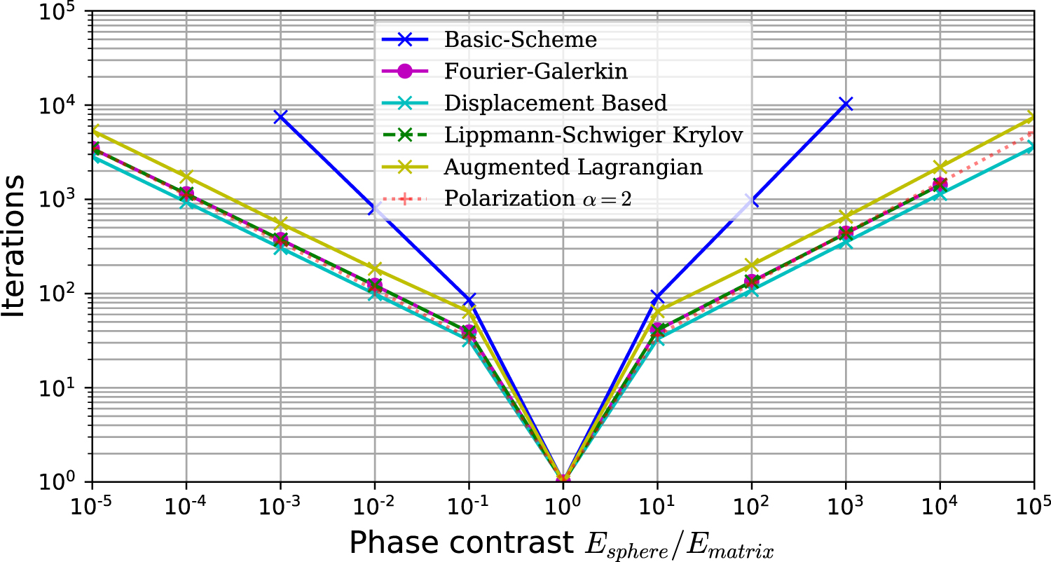
Figure 36. Applications to ultrasonic NDT of materials. Left to right: a photo of an aluminum NDT sample and its corresponding 3D overset computational domain (Amlani and Bruno 2016); temporal snapshots of normalized experimental and FC-simulated displacement fields demonstrating excellent quantitative agreement (Amlani et al 2019b). Reprinted from [Amlani, F., Bruno, O.P., (2016)], Copyright (2016), with permission from Elsevier.
Download figure:
Standard image High-resolution image
5.1.2. Bloch boundary conditions
A second group of works studying problems which does not fulfill the strict RVE periodicity have been recently introduced in FFT frameworks Zhou and Bhattacharya (2021), Segurado and Lebensohn (2021). These studies rely on the use Bloch boundary conditions, that were introduced by Bloch (Bloch 1929) to describe the quantum wave functions of electrons in a crystal lattice. The Bloch–Floquet formalism establishes that for any field u traveling as an harmonic wave in a periodic infinite medium with periodicity L, the value of the field at a point x ∈ (−∞, ∞) should follow

where U(x) is a periodic function with periodicity L, U(x + nL) = U(x) for  , and k and ω correspond to the wave number and frequency respectively. The key idea is introducing the Bloch condition (equation (146)) in the linear momentum balance to study the deformation of an infinite periodic medium with period L in which the periodicity in the displacement field is fulfilled over several cells, Lperiod > L. This periodicity is then prescribed by setting the wave number k in equation (146) as k = 2π/Lperiod. The problem was exploited in Zhou and Bhattacharya (2021) in an static setting, to find bifurcations in the deformation of a non-linear periodic medium. In Segurado and Lebensohn (2021), Bloch conditions were used to study acoustic wave propagation in elastic heterogeneous materials. In particular, an FFT based method was proposed to obtain the dispersion diagram of a periodic heterogeneous material. The accuracy of the method was assessed by comparing with analytical solutions and Fourier series based analysis. The numerical efficiency reached is dependent on the elastic phase contrast, as usual in FFT based approaches, being competitive with FEM for composites or polycrystals. The method was then used to study wave propagation in elastic polycrystals using large 3D RVEs containing hundreds of grains. The simulation allowed to account for the effect of grain size and texture in the wave group velocity.
5.2. Non-uniform grids
Development of FFT algorithms applied to solve problems on non-uniformly sampled data has been the subject of research in the decades after the proposition of the FFT approach by Cooley and Tukey (Cooley and Tukey 1965).
One of the earliest FFT approaches for unevenly spaced data was proposed by Lomb (Lomb 1976) and Scargle (Scargle 1982) for astrophysics applications; this approach is known as the Lomb–Scargle periodogram (Horne and Baliunas 1986, Press and Teukolsky 1988, Press and Rybicki 1989). The working principle of the Lomb–Scargle periodogram is well summarized by Press and Teukolsky (1988), Press and Rybicki (1989) (who have also published the Fortran77 code) and it is recalled below in the case of 1D unevenly sampled data.
Consider N unevenly spaced data points h ≡ h(ti ), i = 1, ..., N. The Lomb–Scargle periodogram involves first computing the mean and variance of the data as:

The Lomb–Scargle normalized periodogram (spectral power as a function of angular frequency ω = 2πξ > 0) is then defined as

where τ is a constant offset that makes PN (ω) completely independent of shifting all the ti 's by any constant. It is defined by the relationship

Lomb (Lomb 1976) showed that the equation for PN (ω) is identical to the equation that one would obtain if one were to estimate the harmonic content of h ≡ h(ti ) via a linear least-squares fitting to the following model:

The advantage of the Lomb–Scargle periodogram that makes it superior to periodic FFT methods is that it weights the data on a 'per point' basis instead of a 'per time interval' basis; the latter induces significant errors for unevenly spaced data that the former avoids. The disadvantage of the Lomb–Scargle periodogram is that it requires 102 N log N iterations in comparison to the N log N iterations for the periodic FFT method. Press and Rybicki (Press and Rybicki 1989) proposed a fast computational approach involving the direct computation of the Lomb–Scargle periodogram.
Many other non-uniform FFT (so called NUFFT or NFFT) approaches different from the Lomb–Scargle periodogram have also been proposed. Interested readers may refer to the following works Bagchi and Mitra (1999), Potts et al (2001), Fessler and Sutton (2003), Greengard and Lee (2004) among others. To the best of our knowledge, none of the non-uniform grid based approaches have been applied to the field of micromechanics, but a remarkable work in a very close area was proposed in Feng et al (2006). In this work the authors define non regular mesh in the physical domain. This mesh is adapted to the current geometry of the microstructure, while maintaining the uniform grid in the computational domain necessary for the FFT computation. This approximation allows to preserve smooth interfaces in the physical domain.
6. Conclusions and future trends
FFT based approaches in micromechanics were first proposed for computational homogenization in the seminal paper (Moulinec and Suquet 1994). This original method, called the basic scheme, was a breakthrough because before that moment almost all the numerical micromechanical approaches were based on the FE method. The reasons for the success of the FFT approach in the field of computational homogenization are (i) its very efficient numerical response, (ii) the reduced memory allocation needs and (iii) the possibility of using 2D/3D images as input data without the requirement of a mesh. Additionally, computational homogenization typically involves evaluating periodic functions, which makes FFT the ideal approach to solve the problem.
The basic scheme presented some limitations such as slow convergence rates for materials with high contrast in properties between phases, which also resulted in a noisy response. The past 30 years have seen a lot of efforts been dedicated to overcome these limitations. These developments have resulted in the creation of tens of different algorithms with improved convergence rates and solution accuracy in comparison to the basic scheme. Nowadays, several high-performance FFT approaches can be found to study the non-linear response of microstructures with arbitrary phase contrast subjected to finite deformations. Moreover, thanks to the advances in computational power, strongly non-linear problems with several millions of degrees of freedom can be computed using FFT approaches in desktop computers without the need of using high performance computational clusters or supercomputers.
With such fast converging and accurate algorithms, the FFT method has become a fundamental tool in micromechanics with a variety of applications to study the mechanical response of composite materials, metal/alloy polycrystals, porous materials, polymers, laminates, concrete, etc. In these studies, FFT has been used to homogenize the response of heterogeneous materials containing linear elastic, viscoelastic or hyperelastic phases as well as a full range of inelastic behaviors such as plasticity, viscoplasticty, damage, etc. In addition, FFT approaches have been used to study fracture and fatigue initiation at the microscale. Applications of the FFT method have also gone beyond the classical micromechanical applications, being used to simulate other micromechanical problems such as dislocation dynamics, strain gradient plasticity, etc. They have also been used to study multi-physics systems involving a strong coupling of the mechanical problem with thermal, electrical, magnetic and pyroelectric problems. In addition, a very interesting application of these methods is their use as a micromechanical solver in concurrent multi-scale frameworks such as the FE–FFT approach where the macroscopic boundary value problem is solved using the FE method and each integration point of the mesh is then solved using an FFT simulation. Finally, they have been successfully employed in synergy with advanced experimental studies involving neutron and synchrotron diffraction and microscopy to (i) gain a comprehensive understanding of the material behavior and (ii) to obtain insight on the material response that is not accessible via experimental studies.
The current challenges that limit the application of FFT approaches in comparison to the FE approach is the requirement of (i) periodicity of the domain and boundary conditions, and (ii) uniformity of the grid. Some promising work has been done toward extending the applicability of the FFT method to solve mechanical problems on non-periodic domains, notably the FC method, which has been presented in the previous section. Finally, the last limitation pointed of FFT approaches is the inability to use non-uniform grids. To that end, motivation can be derived from work done in other physics fields, notably astrophysics and medical imaging where FFT solvers have been developed and applied to treat non-uniformly spaced data. An example of the application of non-uniform grid based FFT approach that is the closest to micromechanical modeling is its use in a phase-field approach (Feng et al 2006) where a moving adaptive mesh is used.
To conclude this work it is interesting to envision what could be the future of the FFT approach. Looking into the continuous growth of the number papers relying on FFT approaches, it is safe to say that FFT approaches in micromechanics are here to stay and their use will be extended in the near future to many new applications, especially with the development of non-periodic and non-uniform grid based FFT approaches. There is still a lot to be done in multi-physics approaches involving the coupling of many problems, for example, the chemo-thermo-mechanical study of batteries, which including phase field damage may involve four different fields coupled by their corresponding PDEs. FFT approaches are also an ideal tool for microscale simulations in concurrent multi-scale modeling and it is possible to exploit them for other problems or simulation frameworks, such as higher order homogenization or micromorphic approaches. Finally, as in any other numerical technique, massive parallelization to deal with extremely large RVEs will be an important topic, following in the footsteps of Chen et al (2019b, 2019a), Zhou and Bhattacharya (2021). This can be relatively easily handled thanks to very efficient open source parallel implementations of the FFT algorithm available nowadays for both MPI or GPU. With respect to extending the FFT method to non-uniform grids, there is a lot of potential for development. Existing approaches such as the phase-field approach by (Feng et al 2006) are designed for applications to specific problems and require pre-processing routines that are as complex as building an FE mesh.
Acknowledgments
Sergio Lucarini acknowledges support from the European Union's Horizon 2020 Marie Skłodowska-Curie Actions through the Project SIMCOFAT (Grant Agreement ID: 101031287). Manas V. Upadhyay is grateful to the European Research Council (ERC) for their support through the European Union's Horizon 2020 Research and Innovation Programme for the project GAMMA (Grant Agreement No. 946959). Javier Segurado acknowledges the European Union's Horizon 2020 Research and Innovation Programme for the Project MOAMMM, Grant Agreement No. 862015, of the H2020-EU.1.2.1.—FET Open Programme and the Spanish Ministry of Science for the Project ADSORBENT, Plan estatal de I+D+i-20019: PID2019-106759GB-I00.
Data availability statement
The data that support the findings of this study are available upon reasonable request from the authors.