
Abstract
This article is devoted to studying the dynamical evolution and orbital stability of compact extrasolar three-planetary system GJ 3138. In this system, all semimajor axes are less than 0.7 au. The modeling of planetary motion is performed using the averaged semi-analytical motion theory of the second order in planetary masses, which the authors construct. Unknown and known with errors orbital elements vary in allowable limits to obtain a set of initial conditions. Each of these initial conditions is applied for the modeling of planetary motion. The assumption about the stability of observed planetary systems allows to eliminate the initial conditions leading to excessive growth of the orbital eccentricities and inclinations and to identify those under which these orbital elements conserve moderate values over the whole modeling interval. Thus, it becomes possible to limit the range of possible values of unknown orbital elements and determine their most probable values in terms of stability.
Export citation and abstract BibTeX RIS
1. Introduction
More than a hundred three-planetary and four-planetary extrasolar systems have been discovered to the present time. The dynamical evolution and orbital stability of these systems require study. Authors have constructed the semi-analytical motion theory of the third order in planetary masses to investigate the orbital evolution of four-planetary systems with moderate orbital eccentricities and inclinations.
The osculating Hamiltonian of the four-planetary problem is written in the Jacobi coordinate system (Murray & Dermott 2000), which is preferable for the study of planetary motion. It is a hierarchical coordinate system in which the position of each following body is determined relative to the barycenter of previously included bodies set. Then, it is expanded into the Poisson series in the small parameter and all orbital elements of the second Poincaré system (Sharlier 1927). This canonical system has only one angular element—mean longitude, which allows to sufficiently simplify an angular part of the series expansion. The ratio of the sum of planetary masses to the star mass plays the role of a small parameter. All orbital elements and mass parameters are conserved symbolically in the series expansion. The series coefficients and degrees of orbital elements are rational numbers with arbitrary precision. It allows eliminating rounding errors in the process of the Hamiltonian construction. The algorithm of the Hamiltonian series expansion is described in detail by authors in Perminov & Kuznetsov (2015).
We applied the Hori–Deprit method (Kholshevnikov 1985; Ferraz-Mello 1988) to construct the Hamiltonian in averaged orbital elements (the averaged Hamiltonian). The essence of any averaging method is to exclude from the osculating Hamiltonian all short-periodic perturbations, defined by terms with fast variables (mean longitudes in our case). The periods of change of fast variables, contrary to slow variables, are comparable to the orbital periods of planets. This approach allows us to sufficiently increase the integration step of the equations of motion in averaged elements. The algorithm of construction of the averaged Hamiltonian and the equations of motion in averaged elements is considered in Perminov & Kuznetsov (2016). The equations of motion are constructed as the Poisson brackets of the averaged Hamiltonian with the corresponding orbital elements. The transformation between osculating and averaged orbital elements is performed by the functions for the change of variables. An application of the constructed four-planetary motion theory to modeling the orbital evolution of the solar system's giant planets is considered by authors in Perminov & Kuznetsov (2018, 2020) for the second and third orders of theory correspondingly.
We relied on the averaged Hamiltonian in the present work, constructed up to the second-order in the small parameter. Higher accuracy of the Hamiltonian expansion is not required because the orbital elements of the extrasolar planetary systems are most often highly uncertain. Here the terms of the first order save the eccentric and oblique Poincaré orbital elements up to the sixth degree, and the terms of the second order-up to the fourth degree.
The orbital elements of extrasolar planetary systems are known from observations with high uncertainy, and some elements are not determined due to the specificity of the observation methods. This work is devoted to the study of the dynamical evolution of the three-planetary extrasolar system GJ 3138. All unknown and known with uncertanties orbital elements are varied within allowable limits to determine the set of initial conditions for the numerical integration of the equations of motion in averaged elements. The limits of change of the orbital elements are determined depending on the initial conditions of the integration. The assumption about the stability of observed planetary systems allows us to exclude the initial conditions leading to excessive orbital eccentricities and inclinations to identify those under which these elements conserve small or moderate values over the modeling interval. Thus, it is possible to narrow the allowable range of unknown orbital elements and determine their most probable values in terms of stability.
2. Properties of the System GJ 3138 and Variation of Orbital Elements
Star GJ 3138 is a red dwarf of spectral type M0V with mass M⋆ = 0.681 M⊙ (in Solar mass) and apparent magnitude mV = 10.877 mag. It is located in the constellation Cetus at a distance d⋆ = 29.9 pc. Two super-Earths and one sub-Neptune (minimal possible masses) orbiting around GJ 3138 were discovered from variations of the radial velocity of the star (Doppler spectroscopy) with the HARPS spectrograph in 2017 as reported in Astudillo-Defru et al. (2017).
The orbital elements and planetary masses of system GJ 3138 are presented in Table 1 together with their uncertainties according to the exoplanet.eu database (Schneider et al. 2011; Astudillo-Defru et al. 2017). Since the planets in system GJ 3138 were discovered via Doppler spectroscopy, only lower limits on their masses Mp are known

where Ip is an unknown inclination of the orbital plane to the sky plane and M is unknown "true" planetary mass. In Table 1 the values of Mp are given in Jupiter's mass MJup. The semimajor axes a, orbital eccentricities e and orbital periods P are known for all planets. Note that planetary system GJ 3138 is compact—the apastron distances do not exceed 1.1 au, considering the maximum possible eccentricities.
Table 1. Known Orbital Elements and Planetary Masses of Extrasolar System GJ 3138
| Planet | Mp (MJup) | a (au) | e | P (days) |
|---|---|---|---|---|
| GJ 3138 c |

| 0.00197 ± 0.0005 |

|

|
| GJ 3138 b | 0.0132 ± 0.0019 | 0.057 ± 0.001 |

| 5.974 ± 0.001 |
| GJ 3138 d |

|

|

|

|
Download table as: ASCIITypeset image
The orbital plane of the outermost planet GJ 3138 d (the most massive and least influenced by two inner planets) is chosen as the reference plane for the planetary motion. Thus, without loss of generality, the orbital inclination Id and the longitude of the ascending node Ωd of the planet GJ 3138 d are equal to 0° at the initial moment of the modeling interval.
The initial values of other orbital elements are set as follows. The initial values of orbital inclination I0 of both inner planets are taken equal and vary from 0° to 35° with a step of 5°. Different configurations of the planetary orbits are achieved by changing the initial values of both the longitudes of the ascending nodes of two inner planets (Ωc , Ωb ) and the arguments of the pericenters of all planets (ωc , ωb and ωd ) with a step of 90° (and additionally 30°). All initial values of the orbital eccentricities are specified to be equal to their minimum, nominal and maximum values from Table 1. Thus there are three sets of initial values of the orbital eccentricities. The planetary masses change simultaneously with the initial values of the orbital inclinations according to Equation (1), and their uncertainties are not taken into account. The initial values of the semimajor axes are nominal and do not vary because their uncertainties are small.
The estimates of the theoretical radii of the convergence for the series representing the equations of motion in the orbital eccentricities Re and inclinations RI are calculated according to Kholshevnikov (2001), Kholshevnikov et al. (2002). If the current values of eccentricities and inclinations e ≤ Re and I ≤ RI in the modeling process, the convergence of the series of the equations of motion and the suitability of the motion theory are guaranteed. In GJ 3138, the condition e ≤ Re corresponds to the planetary orbits that do not intersect. The radii of the convergence are presented in Table 2 for maximum values of the orbital eccentricities and nominal values of the semimajor axes according to Table 1.
Table 2. Theoretical Radii of the Convergence of the Series Representing the Equations of Motion
| Planet | GJ 3138c | GJ 3138 b | GJ 3138 d |
|---|---|---|---|
| Re | 0.66 | 0.38 | 0.66 |
| RI , ° | 80 | 44 | 80 |
Download table as: ASCIITypeset image
3. Results of the Semi-analytical Motion Theory
The equations of motion in averaged orbital elements (based on the averaged Hamiltonian) are numerically integrated by the Gragg–Bulirsch–Stoer method of 7th order (Press et al. 2007; Avdyushev 2015). The modeling interval for the system GJ 3138 is 1 Myr, which corresponds to 300 × 106 revolutions of planet GJ 3138 c around the host star, ande 60 × 106 and 1.4 × 10⁶ revolutions for planets GJ 3138 b and GJ 3138 d respectively. The integration step is 1000 years. The equations of motion are integrated for several tens of seconds on a 3300 MHz Core i7 PC. In some cases, the modeling interval was increased to 10 Myr (see Section 4).
For each initial value of the orbital inclination I0, of two inner planets (7 values) and three sets of initial orbital eccentricities, 1024 variants of the orbital evolution are simulated. These variants are determined by different combinations of the initial longitudes of the ascending nodes (Ωc , Ωb ) and the initial arguments of the pericenters (ωc , ωb , ωd ).
Tables 3–5 present the maximum values of the averaged orbital eccentricities  and inclinations
  achieved on the modeling interval by orbits of planets GJ 3138 b, c and d correspondingly. Depending on the initial values of the orbital eccentricities e0 and inclinations of two inner planets I0, each tabular cell contains the range of the highest values
  and
and  determined for all initial combinations of the arguments of the pericenters ω0 and the longitudes of the ascending nodes Ω0. Columns marked as M in Tables 3 and 4 contain the values of planetary masses corresponding to the initial value of orbital inclination I0 (planets GJ 3138c and b). If the inclination of the orbital plane to the plane of the sky Ip
= 90° − I0, then planetary mass
determined for all initial combinations of the arguments of the pericenters ω0 and the longitudes of the ascending nodes Ω0. Columns marked as M in Tables 3 and 4 contain the values of planetary masses corresponding to the initial value of orbital inclination I0 (planets GJ 3138c and b). If the inclination of the orbital plane to the plane of the sky Ip
= 90° − I0, then planetary mass  . The mass of planet GJ 3138 d is set equal to its nominal value according to Table 1.
Table 3. Maximum Values of the Averaged Orbital Eccentricities and Inclinations of Planet GJ 3138 c
| e0 | 0.06 | 0.19 | 0.37 | ||||
|---|---|---|---|---|---|---|---|
| I0 (°) | M (MJup) |

|

|

|

|

|

|
| 0 | 0.005600 | 0.06−0.10 | 0 | 0.19−0.28 | 0 | 0.38−0.57 | 0 |
| 5 | 0.005621 | 0.06−0.10 | 11 | 0.19−0.28 | 12 | 0.38−0.57 | 15.5 |
| 10 | 0.005686 | 0.06−0.11 | 22 | 0.19−0.31 | 23 | 0.38−0.59 | 29 |
| 15 | 0.005798 | 0.06−0.14 | 33 | 0.19−0.36 | 35 | 0.38−0.64 | 42 |
| 20 | 0.005959 | 0.06−0.44 | 45 | 0.20−0.57 | 47 | 0.38−0.8 | 60 |
| 30 | 0.006466 | 0.06−0.75 | 79 | 0.2−0.9 | 72 | 0.4−1 | 75 |
| 35 | 0.006836 | 0.06−1 | 82 | 0.2−1 | 85 | 0.4−1 | >90 |
Note. The values of the orbital eccentricities and inclinations, which exceed the radii of convergence, are marked by bold font.
Download table as: ASCIITypeset image
Table 4. Maximum Values of the Averaged Orbital Eccentricities and Inclinations of Planet GJ 3138 b
| e0 | 0.04 | 0.11 | 0.22 | ||||
|---|---|---|---|---|---|---|---|
| I0 (°) | M (MJup) |

|

|

|

|

|

|
| 0 | 0.013200 | 0.04–0.05 | 0 | 0.11–0.14 | 0 | 0.22–0.29 | 0 |
| 5 | 0.013250 | 0.04–0.05 | 6 | 0.11–0.14 | 6 | 0.22–0.29 | 6 |
| 10 | 0.013404 | 0.04–0.05 | 11 | 0.11–0.15 | 11 | 0.22–0.29 | 12 |
| 15 | 0.013666 | 0.04–0.06 | 17 | 0.11–0.15 | 17 | 0.22–0.31 | 18 |
| 20 | 0.014047 | 0.04–0.14 | 22 | 0.11–0.24 | 23 | 0.22–0.38 | 25 |
| 30 | 0.015242 | 0.04–0.35 | 33 | 0.11–0.47 | 34 | 0.22–0.5 | 36 |
| 35 | 0.016114 | 0.04–0.5 | 39 | 0.11–0.6 | 40 | 0.22–0.6 | 40 |
Note. The values of the orbital eccentricities, which exceed the radius of convergence, are marked by bold font.
Download table as: ASCIITypeset image
Table 5. Maximum Values of the Averaged Orbital Eccentricities and Inclinations of Planet GJ 3138 d
| e0 | 0.11 | 0.32 | 0.52 | |||
|---|---|---|---|---|---|---|
| I0 (°) |

|

|

|

|

|

|
| 0 | 0.11 | 0 | 0.32 | 0 | 0.52 | 0 |
| 5 | 0.1102 | 1.2 | 0.3203 | 1.3 | 0.5205 | 1.4 |
| 10 | 0.1102 | 2.5 | 0.3203 | 2.6 | 0.5206 | 2.9 |
| 15 | 0.1102 | 3.8 | 0.3204 | 4.0 | 0.5223 | 4.5 |
| 20 | 0.1108 | 5.2 | 0.3214 | 5.8 | 0.5242 | 6.0 |
| 30 | 0.1119 | 8.3 | 0.3230 | 9.0 | 0.5230 | 10.5 |
| 35 | 0.1180 | 11.5 | 0.3282 | 12.2 | 0.5270 | 13.3 |
Download table as: ASCIITypeset image
For greater clarity, the modeling results are presented in Figures 1–4, that show maximum achievable values (on the entire modeling interval) of the averaged orbital eccentricities of two inner planets GJ 3138 c and GJ 3138 b for nominal initial values of the orbital eccentricities. The initial inclinations I0 of two inner planets are 15° (Figure 1), 20° (Figure 2), 30° (Figure 3) and 35° (Figure 4). Figures 5 (I0 = 15°) and 6(I0 = 35°) present maximum achievable values of the averaged orbital inclinations of planets GJ 3138 c and GJ 3138 b (in degrees). The variation step of initial values of ωc , ωb , ωd and Ωc , Ωd is equal to 90°. Initial values of Ωb are marked along the horizontal axis on both panels for each figure, and initial values of ωc —along the vertical axis. Each small square in the figures corresponds to specific initial values of Ωb (horizontal side) and ωb (vertical). Also in each small square inteaitial values of ωd change vertically. The range of maximum values of the averaged eccentricities in Figures 1–4 corresponds to that given in the Tables 3 and 4. Maximum achievable values of the orbital eccentricity and inclination of planet GJ 3138 d change slightly with increasing initial inclinations I0 of planets c and b (see Table 5). The range of maximum values of the averaged orbital inclinations in Figures 5–6 corresponds to the range from I0 to the value given in Tables 3 and 4. The shown behavior of the orbital elements is qualitatively preserved for the minimum and maximum initial values of the orbital eccentricities. The arguments of the pericenters and the longitudes of the ascending nodes of all planets change in the range from 0° to 360° without librations for all considered initial conditions.
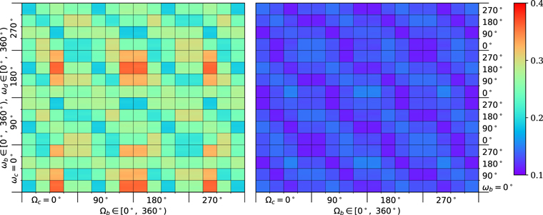
Figure 1. Maximum values of the averaged orbital eccentricities of planets GJ 3138 c (left) and b (right) for nominal initial values of orbital eccentricities; initial orbital inclinations of planets c and b are 15°.
Download figure:
Standard image High-resolution image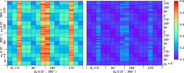
Figure 2. Maximum values of the averaged orbital eccentricities of planets GJ 3138 c (left) and b (right) for nominal initial values of orbital eccentricities; the initial orbital inclinations of planets c and b are 20°.
Download figure:
Standard image High-resolution image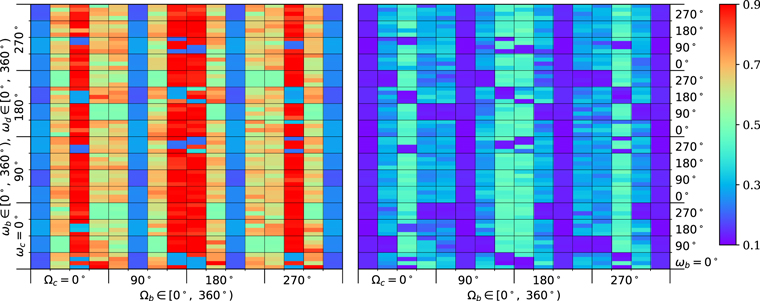
Figure 3. Maximum values of the averaged orbital eccentricities of planets GJ 3138 c (left) and b (right) for nominal initial values of orbital eccentricities; the initial orbital inclinations of planets c and b are 30°.
Download figure:
Standard image High-resolution image
Figure 4. Maximum values of the averaged orbital eccentricities of planets GJ 3138 c (left panel) and b (right panel) for nominal initial values of orbital eccentricities; the initial inclinations of planets c and b are 35°.
Download figure:
Standard image High-resolution image
Figure 5. Maximum values of the averaged orbital inclinations (in degrees) of planets GJ 3138 c (left) and b (right) for nominal initial values of orbital eccentricities; the initial inclinations of planets c and b are 15°.
Download figure:
Standard image High-resolution image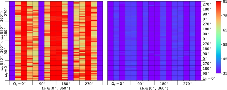
Figure 6. Maximum values of the averaged orbital inclinations (in degrees) of planets GJ 3138 c (left) and b (right) for nominal initial values of orbital eccentricities; the initial inclinations of planets c and b are 35°.
Download figure:
Standard image High-resolution imageAs seen from Tables 3–5 and Figures 1–6, there is the set of initial combinations of the arguments of the pericenters and the longitudes of the ascending nodes providing the stability of dynamical evolution of the planetary system. At the same time, there are initial conditions that lead to excessive growth of the orbital eccentricities and possibly to flips of the orbits (transitions between prograde and retrograde motion). Note that flips and extreme values of the eccentricities (close to 1) can be manifested as an artifact of the analytical theory since such values of inclinations and eccentricities exceed the radii of the convergence. In this case, the real orbital evolution, including the real presence of flips, can be studied only by using numerical methods.
More detailed maps of the distribution of maximum values of the averaged orbital eccentricities and inclinations are shown in Figures 7 (I0 = 15°) and 8 (I0 = 20°). The variation step of initial values of ωb , ωd and Ωb is less than or equal to 30°, and initial values of ωc and Ωc are equal to 0°. The orbital evolution for such initial conditions is simulated for all values of I0 considered above and for all sets of the initial orbital eccentricities. There are 1728 combinations of initial values of ωb , ωd , and Ωb for each value of I0 together with a specific set of the orbital eccentricities.

Figure 7. Maximum values of averaged orbital eccentricities of planets GJ 3138 c (top left panel) and b (top right panel), averaged orbital inclinations of planets GJ 3138 c (bottom left panel) and b (bottom right panel) for nominal initial values of orbital eccentricities and initial inclinations of planets c and b are 15°.
Download figure:
Standard image High-resolution image
Figure 8. Maximum values of averaged orbital eccentricities of planets GJ 3138 c (top left panel) and b (top right panel), averaged orbital inclinations of planets GJ 3138 c (bottom left panel) and b (bottom right panel) for nominal initial values of orbital eccentricities and initial inclinations of planets c and b are 20°.
Download figure:
Standard image High-resolution imageFor I0 ≤ 15°, the distribution of the maximum values of the orbital eccentricities qualitatively corresponds to that displayed in Figure 7. By increasing the value of initial inclination (I0 ≥ 20°), the areas of significant growth in eccentricity of the orbit of planet GJ 3138 c (top left panel of Figure 7 or left panel of Figure 1) merge together into vertical lines with larger maximum eccentricity (top left panel of Figure 8 or left panel of Figure 2). The behavior of the areas with significant growth in the eccentricity of the orbit of planet GJ 3138 b is similar to planet GJ 3138 c for I0 ≥ 20°.
4. Accuracy of Integration of the Averaged Equations of Motion
We evaluated the total system energy on each step of the integration by substituting current values of the orbital elements to the Hamiltonian expansion. The relative accuracy of the conservation for the total system energy ΔE is defined as the relative difference between initial system energy E0 and its current value E

The conservation of the total system energy means that the phase trajectories, which correspond to the exact and approximate solutions, are on the same phase surface. However, it does not mean that phase trajectories are close to each other.
In this case, when the variation step of the arguments of the pericenters and the longitudes of the ascending nodes equals 90°, we set the precision of integration by the Gragg–Bulirsch–Stoer method to ε = 10−7 (ε is a difference between the approximate solutions at the current step and the previous). If the variation step is 30°, we set ε = 10−9. The first case corresponds to ΔE ∈ [10−7, 10−4] at the end of the integration interval of 1 Myr. The second case corresponds to ΔE ∈ [10−8, 10−5] at the end of the same interval. The left borders of the above ranges are realized when the values of orbital eccentricities and inclinations remain close to the initial ones over the entire integration interval. Otherwise, the orbital eccentricities close to 1 and inclinations close to 90° can realize the values close to the right borders. If ε = 10−12, then ΔE ≲ 10−10, but the integration time increases significantly.
Let us consider the results of the integration with different precisions ε = 10−7, 10−9, 10−12. As an example we take the following initial conditions: I0 = 15°, 30°; Ωb = 180°, ωd = 90°; other arguments and nodes equal to 0°; all orbital eccentricities take their nominal values. Figures 9, 10 (I0 = 15°) and 11, 12 (I0 = 30°) show the results of the integration with ε = 10−7 (red lines), ε = 10−9 (blue lines) and ε = 10−12 (black lines).

Figure 9. Evolution of the averaged orbital eccentricities of planets GJ 3138 c (red and black solid lines), GJ 3138 b (dotted lines) and GJ 3138 d (gray line) over time intervals 1 and 10 Myr for different values of the precision of integration ε. Initial orbital inclinations of planets c and b, I0 = 15°.
Download figure:
Standard image High-resolution image
Figure 10. Evolution of the averaged orbital inclinations of planets GJ 3138 c (red and black solid lines), b (dotted lines) and d (gray line) over time intervals 1 and 10 Myr for different values of the precision of integration ε. Initial orbital inclinations of planets c and b, I0 = 15°.
Download figure:
Standard image High-resolution image
Figure 11. Evolution of the averaged orbital eccentricities of planets GJ 3138 c (red, blue and black solid lines), b (dotted lines) and d (gray line) over time intervals 1 and 10 Myr for different values of the precision of integration ε. Initial orbital inclinations of planets c and b, I0 = 30°.
Download figure:
Standard image High-resolution image
Figure 12. Evolution of the averaged orbital inclinations of planets GJ 3138 c (red, blue and black solid lines), b (dotted lines) and d (gray line) over time intervals 1 and 10 Myr for different values of the precision of integration ε. Initial orbital inclinations of planets c and b, I0 = 30°.
Download figure:
Standard image High-resolution imageIn Figures 9 and 10, the evolution of the averaged orbital eccentricities and inclinations of all planets is given over time interval 10 Myr. A good agreement is seen between the integration results obtained with ε = 10−7 and ε = 10−12 if I0 = 15° (and less). Figure 11 shows that the averaged orbital eccentricities of two inner planets increase extremely after about 0.5 Myr for ε = 10−7 and ε = 10−9 if I0 = 30°. If ε = 10−12 the averaged orbital eccentricities of two inner planets begin to increase after about 4 Myr. The box in Figure 11 displays the evolution of the averaged orbital eccentricities over a time interval up to 0.1 Myr. Figure 12 depicts the evolution of the averaged orbital inclinations for I0 = 30°. Note that as the orbital eccentricities of two inner planets increase significantly, the orbital inclinations of ones decrease slightly (see Figures 11 and 12).
5. Comparison with Direct Numerical Integration
The direct numerical simulation of the orbital evolution of planetary system GJ 3138 is performed by the symplectic Wisdom–Holman method implemented in the REBOUND code (program WHFast) by Rein & Tamayo (2015). The time interval of the numerical integration is 1 Myr, and the integration step is 0.1 day. For several sets of initial conditions, the direct numerical integration of Newtonian equations of motion and the semi-analytical motion theory are compared.
Figure 13 shows the evolution of the orbital eccentricities of planets GJ 3138 c (data marked in red), b (blue) and d (gray) for different initial conditions. The solid lines and the dots correspond to the results of the semi-analytical motion theory and the numerical simulation respectively. The left column of Figure 13 depicts results for the following initial arguments of the pericenters and longitudes of the ascending nodes ωc = 0°, ωb = 150°, ωd = 210° and Ωb = 30°, Ωc = Ωd = 0°. The results presented in the right column of this figure correspond to ωc = 0°, ωb = 30°, ωd = 30° and Ωb = 180°, Ωc = Ωd = 0°. The value of I0 varies as marked in Figures 13(a)–(j). Evolution of the orbital inclinations for both sets of initial conditions is shown in Figure 14.

Figure 13. Evolution of the orbital eccentricities of planets GJ 3138 c (red solid line and red dots), b (blue solid line and blue dots) and d (gray solid line) over time intervals 0.2 and 1 Myr for different initial conditions. Solid lines correspond to results of semi-analytical motion theory, dots—the direct numerical integration.
Download figure:
Standard image High-resolution image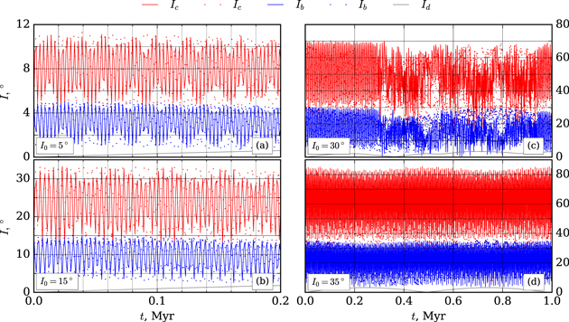
Figure 14. Evolution of the orbital inclinations of planets GJ 3138 c (red solid line and red dots), b (blue solid line and blue dots) and d (gray solid line) over time intervals 0.2 and 1 Myr for different initial conditions. Solid lines correspond to results of semi-analytical motion theory, dots—the direct numerical integration.
Download figure:
Standard image High-resolution imageAccording to Figure 13, the results of the numerical simulation and the semi-analytical motion theory are qualitatively the same for the first set of initial conditions (for each value of I0). Shown behavior of the orbital eccentricities of all planets persists over the whole interval of the simulation. This also applies to the behavior of the orbital eccentricities for the second set of initial conditions up to I0 = 15°. Note that if I0 = 20°, the periods of change of the orbital eccentricities of planets GJ 3138 b and c, determined by two methods, differ significantly, but the limits of change—slightly (see Figure 13(f)). For I0 ≥ 30°, an increase in the orbital eccentricity of planet GJ 3138 c in the process of numerical simulation occurs immediately according to Figures 13(h) and (j). The modeling within the framework of the semi-analytical motion theory exhibits an increase in the orbital eccentricity after some time interval. In some cases, like what is shown in Figure 13(j), the behavior of the orbital eccentricity of planet GJ 3138 c is different for the numerical simulation and the semi-analytical motion theory (see also Figures 3 and 4).
The limits of change (and amplitudes) of the orbital inclinations increase with increasing I0 according to Figure 14.
Let us compare the results obtained by WHFast integrator with the IAS15 one (which stands for Integrator with Adaptive Step-size control, 15th order, implemented in the REBOUND code). IAS15 is an adaptive integrator that chooses timestep automatically. The accuracy of this integrator is 10−9 by default. The integration time is 80 kyr with a nominal timestep of 0.1 day for both WHFast and IAS15 integrators. Figure 15 shows the comparison of the orbital evolution of eccentricities and inclinations obtained by the WHFast integrator (solid lines) with the results of IAS15 integrator (dots). Initial values of the orbital elements are the following: ωc = 0°, ωb = ωd = 30°, Ωc = Ωd = 0°, Ωb = 180°, mean longitudes are zero, orbital eccentricities are nominal.
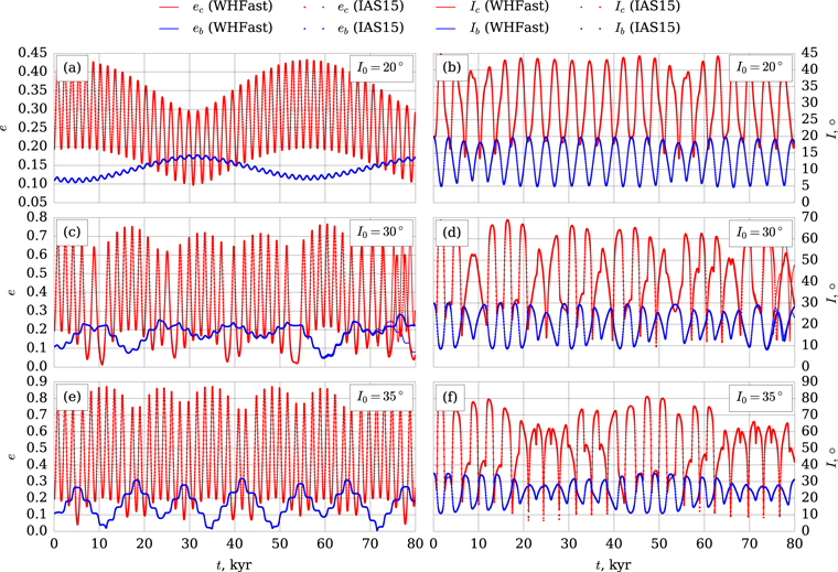
Figure 15. Evolution of the orbital eccentricities (left) and inclinations (right) of planets GJ 3138 c (red solid line and red dots) and b (blue solid line and blue dots) over a time interval of 80 kyr for nominal initial values of eccentricities and different initial values of inclinations. Solid lines correspond to results of WHFast integrator, dots—IAS15 integrator.
Download figure:
Standard image High-resolution imageThe integration process (over time intervals up to 0.1 Myr) takes about 15 hours with the IAS15 integrator and about 10 minutes with the WHFast integrator for a 3300 MHz Core i7 PC. Figure 15 affirms that the data obtained by both integrators are in excellent correlation over time intervals up to 80 kyr. Note, however, that if I0 = 30° the results obtained by WHFast and IAS15 integrators begin to diverge after about 75 kyr as seen from Figures 15(c) and (d). In this case the value of MEGNO (see Section 6.1) does not exceed 2.01 at the end of the modeling interval. Thus, this difference can be explained by using different integrators, but not chaotic motion. Since such differences are insignificant for small initial orbital inclinations (I0 ≤ 20°), it is more efficient to use the WHFast integrator, which is less accurate but faster.
6. Chaotic Properties of the Planetary System GJ 3138
6.1. MEGNO Indicator
As shown in Figure 11, the instability detected with the averaged equations of motion depends on the accuracy of the used integrator. To check that the evolution of the planetary system is chaotic, we evaluate the MEGNO indicator (see, for example, Goździewski et al. 2001 and Goździewski et al. 2008), which stands for Mean Exponential Growth factor of Nearby Orbits. This indicator is similar to the maximal Lyapunov exponent and is a measure of chaos in dynamic systems.
The MEGNO indicator  is implemented in the REBOUND code for WHFast numerical integrator. We calculated MEGNO for the following set of initial conditions: I0 ∈ {5°, 10°, 15°, 20°, 30°, 35°}, Ωc
and Ωb
vary with step of 90°, Ωd
= 0°, mean longitudes are zero, and orbital eccentricities are nominal. Two sets of initial values of the arguments of the pericenters are ω1 = {ωc
= ωb
= ωd
= 0°} and ω2 ={ωc
= ωb
= 90°, ωd
= 0°}. Time interval of the integration is 1 Myr.
is implemented in the REBOUND code for WHFast numerical integrator. We calculated MEGNO for the following set of initial conditions: I0 ∈ {5°, 10°, 15°, 20°, 30°, 35°}, Ωc
and Ωb
vary with step of 90°, Ωd
= 0°, mean longitudes are zero, and orbital eccentricities are nominal. Two sets of initial values of the arguments of the pericenters are ω1 = {ωc
= ωb
= ωd
= 0°} and ω2 ={ωc
= ωb
= 90°, ωd
= 0°}. Time interval of the integration is 1 Myr.
If I0 ≤ 15°, then  for all initial conditions. It means that the planetary motion is quasi-periodic and initial conditions are non-chaotic. Table 6 contains
  and maximum achievable values of the orbital eccentricities for planets GJ 3138 c and GJ 3138 b obtained by the WHFast integrator (
 ,
,  ) and semi-analytical motion theory (
 ,
,  ). Semi-analytical results (
 ,
,  ) obtained by the Gragg–Bulirsch–Stoer method are of 7th order (see Figures 2–4). It is seen that with increasing I0 (and as a consequence the relative inclination of two inner planets), the chaoticity of the planetary motion and the number of chaotic initial conditions increases. The values of
  that correspond to chaotic initial conditions are marked in Table 6 by bold font. If I0 ≤ 20°, then
  and
and  for all initial conditions.
Table 6. The Values of MEGNO Indicator and Maximum Achievable Values of the Orbital Eccentricities of Planets GJ 3138 c and GJ 3138 b
| Ωc | Ωb | ωi | I0 = 20° | I0 = 30° | I0 = 35° | ||||||||||||
|---|---|---|---|---|---|---|---|---|---|---|---|---|---|---|---|---|---|

|

|

|

|

|

|

|

|

|

|

|

|

|

|

| |||
| 0° | 0° | ω1 | 0.193 | 0.193 | 0.145 | 0.145 | 2.0 | 0.193 | 0.193 | 0.146 | 0.146 | 2.0 | 0.194 | 0.193 | 0.147 | 0.146 | 2.0 |
| ω2 | 0.189 | 0.191 | 0.143 | 0.144 | 2.0 | 0.189 | 0.191 | 0.143 | 0.143 | 2.0 | 0.189 | 0.191 | 0.143 | 0.143 | 2.0 | ||
| 0° | 90° | ω1 | 0.296 | 0.290 | 0.133 | 0.132 | 1.9 | 0.487 | 0.631 | 0.156 | 0.225 | 1.9 | 0.605 | 0.703 | 0.205 | 0.280 | 75 |
| ω2 | 0.272 | 0.274 | 0.134 | 0.134 | 2.0 | 0.423 | 0.645 | 0.162 | 0.285 | 57 | 0.590 | 0.893 | 0.185 | 0.471 | 73 | ||
| 0° | 180° | ω1 | 0.427 | 0.428 | 0.181 | 0.148 | 1.9 | 0.805 | 0.276 | 0.340 | 0.113 | 54 | 0.874 | 0.308 | 0.347 | 0.118 | 157 |
| ω2 | 0.377 | 0.487 | 0.117 | 0.152 | 58 | 0.736 | 0.875 | 0.114 | 0.437 | 1.5 | 0.872 | 0.949 | 0.111 | 0.467 | 85 | ||
| 0° | 270° | ω1 | 0.295 | 0.289 | 0.133 | 0.132 | 1.9 | 0.487 | 0.904 | 0.156 | 0.440 | 1.9 | 0.617 | 0.700 | 0.215 | 0.348 | 67 |
| ω2 | 0.271 | 0.272 | 0.134 | 0.132 | 2.0 | 0.431 | 0.666 | 0.149 | 0.296 | 3.5 | 0.618 | 0.754 | 0.203 | 0.426 | 72 | ||
| 90° | 0° | ω1 | 0.291 | 0.287 | 0.132 | 0.131 | 1.9 | 0.487 | 0.732 | 0.155 | 0.319 | 1.9 | 0.573 | 0.698 | 0.170 | 0.285 | 53 |
| ω2 | 0.271 | 0.271 | 0.134 | 0.133 | 2.0 | 0.424 | 0.693 | 0.162 | 0.308 | 14 | 0.625 | 0.700 | 0.208 | 0.275 | 76 | ||
| 90° | 90° | ω1 | 0.190 | 0.191 | 0.144 | 0.145 | 2.0 | 0.190 | 0.192 | 0.145 | 0.145 | 2.0 | 0.190 | 0.192 | 0.145 | 0.146 | 2.0 |
| ω2 | 0.189 | 0.190 | 0.143 | 0.143 | 2.0 | 0.189 | 0.189 | 0.143 | 0.143 | 2.0 | 0.189 | 0.189 | 0.142 | 0.142 | 2.0 | ||
| 90° | 180° | ω1 | 0.293 | 0.287 | 0.134 | 0.133 | 1.6 | 0.482 | 0.762 | 0.159 | 0.360 | 1.9 | 0.577 | 0.917 | 0.175 | 0.495 | 79 |
| ω2 | 0.270 | 0.272 | 0.134 | 0.133 | 2.0 | 0.425 | 0.661 | 0.150 | 0.294 | 2.9 | 0.618 | 0.616 | 0.220 | 0.227 | 89 | ||
| 90° | 270° | ω1 | 0.421 | 0.434 | 0.175 | 0.147 | 1.8 | 0.792 | 0.889 | 0.303 | 0.364 | 54 | 0.876 | 0.305 | 0.327 | 0.117 | 41 |
| ω2 | 0.396 | 0.474 | 0.118 | 0.136 | 50 | 0.736 | 0.849 | 0.116 | 0.473 | 2.6 | 0.872 | 0.960 | 0.113 | 0.544 | 35 | ||
| 180° | 0° | ω1 | 0.421 | 0.431 | 0.172 | 0.150 | 1.9 | 0.781 | 0.281 | 0.296 | 0.128 | 57 | 0.881 | 0.305 | 0.339 | 0.117 | 37 |
| ω2 | 0.388 | 0.577 | 0.110 | 0.220 | 41 | 0.736 | 0.884 | 0.114 | 0.415 | 1.8 | 0.872 | 0.963 | 0.112 | 0.543 | 71 | ||
| 180° | 90° | ω1 | 0.291 | 0.285 | 0.133 | 0.133 | 1.9 | 0.467 | 0.638 | 0.144 | 0.277 | 1.9 | 0.579 | 0.986 | 0.193 | 0.408 | 92 |
| ω2 | 0.271 | 0.274 | 0.134 | 0.134 | 2.0 | 0.422 | 0.715 | 0.169 | 0.327 | 21 | 0.566 | 0.724 | 0.172 | 0.299 | 81 | ||
| 180° | 180° | ω1 | 0.190 | 0.190 | 0.145 | 0.145 | 2.0 | 0.190 | 0.190 | 0.145 | 0.145 | 2.0 | 0.190 | 0.190 | 0.145 | 0.145 | 2.0 |
| ω2 | 0.189 | 0.191 | 0.143 | 0.144 | 2.0 | 0.189 | 0.191 | 0.143 | 0.143 | 2.0 | 0.189 | 0.191 | 0.143 | 0.144 | 2.0 | ||
| 180° | 270° | ω1 | 0.291 | 0.286 | 0.133 | 0.132 | 1.9 | 0.486 | 0.707 | 0.157 | 0.299 | 1.9 | 0.579 | 0.919 | 0.185 | 0.459 | 76 |
| ω2 | 0.271 | 0.272 | 0.134 | 0.132 | 2.0 | 0.427 | 0.606 | 0.150 | 0.265 | 3.6 | 0.628 | 0.985 | 0.214 | 0.519 | 91 | ||
| 270° | 0° | ω1 | 0.291 | 0.289 | 0.132 | 0.131 | 1.9 | 0.492 | 0.727 | 0.156 | 0.324 | 1.9 | 0.561 | 0.766 | 0.188 | 0.346 | 84 |
| ω2 | 0.275 | 0.274 | 0.134 | 0.133 | 2.0 | 0.443 | 0.684 | 0.149 | 0.293 | 1.9 | 0.578 | 0.963 | 0.191 | 0.561 | 86 | ||
| 270° | 90° | ω1 | 0.422 | 0.429 | 0.175 | 0.148 | 1.9 | 0.804 | 0.278 | 0.318 | 0.115 | 73 | 0.874 | 0.306 | 0.328 | 0.117 | 44 |
| ω2 | 0.369 | 0.497 | 0.111 | 0.180 | 69 | 0.735 | 0.916 | 0.113 | 0.463 | 1.7 | 0.871 | 0.983 | 0.111 | 0.517 | 10 | ||
| 270° | 180° | ω1 | 0.293 | 0.288 | 0.134 | 0.133 | 1.9 | 0.484 | 0.912 | 0.155 | 0.417 | 1.9 | 0.727 | 0.662 | 0.284 | 0.252 | 56 |
| ω2 | 0.275 | 0.275 | 0.134 | 0.133 | 2.0 | 0.443 | 0.584 | 0.149 | 0.223 | 3.7 | 0.574 | 0.654 | 0.171 | 0.298 | 53 | ||
| 270° | 270° | ω1 | 0.190 | 0.192 | 0.144 | 0.145 | 2.0 | 0.190 | 0.192 | 0.145 | 0.145 | 2.0 | 0.190 | 0.192 | 0.145 | 0.146 | 1.9 |
| ω2 | 0.192 | 0.192 | 0.145 | 0.144 | 2.0 | 0.192 | 0.192 | 0.145 | 0.144 | 2.0 | 0.192 | 0.192 | 0.145 | 0.145 | 2.0 | ||
Note. The values of MEGNO that correspond to chaotic initial conditions are marked by bold font.
Download table as: ASCIITypeset image
6.2. Lidov–Kozai Resonance
Lidov–Kozai secular resonance is coupled periodic variations of the orbital eccentricity and inclination of an orbiting body, which is caused by the presence of an inclined outer perturber. Librations of the argument of the pericenter ω of orbiting body arise in the presence of Lidov–Kozai resonance. There are two integrals of motion connected with Lidov–Kozai resonance (Shevchenko 2017)

and

If 0 ≤ c1 ≤ 3/5 and c2 < 0, the argument of the pericenter ω librates around 90° or 270°. If 0 ≤ c1 ≤ 1 and c2 > 0, it corresponds to the case of circulating ω.
Let us introduce the relative inclination Irel of orbits GJ 3138 c and GJ 3138 b

Starting from I0 = 20°, initial values of relative inclination Irel can reach 40° and above depending on initial values of Ωc
and Ωb
. If Irel > Icrit ≈ 39 23, the value of c1 < 3/5 and Lidov–Kozai resonance becomes possible (if c2 > 0).
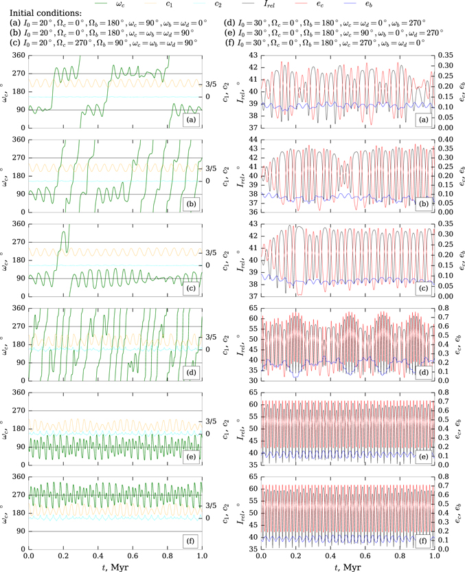
Figure 16 features the examples of orbital evolution of the argument of the pericenter ωc and the orbital eccentricity ec of the innermost planet GJ 3138 c, the orbital eccentricity eb of planet GJ 3138 b, the relative inclination Irel of two inner planets and two integrals of motion c1 and c2 over time intervals up to 1 Myr for different initial conditions. All data were obtained by direct numerical integration (program WHFast). We can distinguish the following variants of ωc evolution depending on the initial conditions.
- 1.
- 2.Transitions between librations around 90° and 270° (see Figures 16(a) and (c)).
- 3.Exit from resonance (see Figure 16(b)).
- 4.Non-resonant evolution (see Figure 16(d)).
The relative inclination Irel and eccentricity ec change in antiphase for all initial conditions.
Figure 16. Evolution of the argument of the pericenter of GJ 3138 c orbit (green line), its eccentricity (red line), the orbital eccentricity of planet GJ 3138 b (blue line), the relative inclination of planets GJ 3138 c and b (black line) and two integrals of motion (orange and cyan lines) over time interval up to 1 Myr for different initial conditions. Initial values of orbital eccentricities are nominal.
Download figure:
Standard image High-resolution image
7. Discussion
If the initial orbital inclinations of both inner planets I0 ≤ 15°, the planetary system GJ 3138 is fully stable on time intervals up to 1 Myr for all initial values of the orbital eccentricities, longitudes of the ascending nodes and the arguments of the pericenters. Wherein the maximum achievable values of the orbital eccentricities and inclinations  (see the radii of the convergence in Table 2).
Figure 1 exhibits some symmetry in the distribution of maximum orbital eccentricities, namely each large square (4 by 4 small squares) contains a distribution similar to that shown in Figure 7 with some offset in the longitudes of the ascending nodes and the arguments of the pericenters. The combinations of the initial angles (nodes and pericenters) corresponding to the maximum increase in the averaged orbital eccentricity of planet GJ 3138 c satisfy the condition  . At the same time, the maximum increase in the averaged orbital eccentricity of planet GJ 3138 b is realized for the condition
  . As the initial orbital inclination I0 increases, these regions expand along the direction
  , and the dependence on the arguments of the pericenters (ωc
and ωb
) weakens.
, and the dependence on the arguments of the pericenters (ωc
and ωb
) weakens.
If I0 = 20°, then  for planets GJ 3138 c and b in the case of any initial values of the orbital eccentricities. The maximum increase in the averaged orbital eccentricities of both inner planets occurs if
  . Suppose the ascending nodes of these two orbits are located on a straight line and opposite from each other. In that case, the maximum value of averaged orbital eccentricities can reach values up to 0.6 (see Figure 2).
In the case of I0 > 20°, there are the initial conditions leading to substantial growth in the orbital eccentricities of planet GJ 3138 c (up to values close to 1). The direct numerical integration confirms an increase in the orbital inclination of planet GJ 3138 c up to values close to 90°. Thus, the orbital flips of the inner planet are quite possible. At the same time, in this case, the areas of orbital stability are partly conserved. Also, the semi-analytical motion theory results must be refined by direct numerical simulation for large values of the initial orbital inclination (I0 = 35°). The maximum increase in the averaged orbital eccentricities of two inner planets occurs for initial values of the longitudes of the ascending nodes ![$\left({{\rm{\Omega }}}_{b}-{{\rm{\Omega }}}_{c}\right)\in \left[90^\circ ,270^\circ \right]$](https://content.cld.iop.org/journals/1674-4527/22/1/015007/revision3/raaac32b5ieqn65.gif) .
.
For all values of I0, the maximum increase in orbital eccentricities of both inner planets occurs if the initial value of  is close to 180°. If
  , orbital planes of both inner planets coincide, and the amplitudes of orbital inclinations do not exceed tenths of a degree.
Note that the orbital motion of planet GJ 3138 d is stable for all initial conditions and em , Im < Re , RI .
The comparison of semi-analytical motion theory with the results of direct numerical integration shows their good agreement for most of the initial conditions. The comparison of different numerical methods of integration confirms the qualitative correspondence of the obtained results.
If the initial value of orbital inclinations of two inner planets I0 ≤ 15°, the value of MEGNO does not exceed 2 over 1 Myr. With increasing I0, the number of initial conditions leading to chaotic evolution of planetary system increases.
If I0 ≥ 20°, the initial conditions leading to Lidov–Kozai resonance appears. If I0 = 20°, conditions for Lidov–Kozai resonance arise for the following initial values of orbital elements: Ωc − Ωb = 180° and ωc = ωb ≠ 0°, 180°. However, there is no capture to the resonance for the whole time interval of 1 Myr (see Figures 16(a)–(c)), since the conditions 0 ≤ c1 ≤ 3/5 and c2 < 0 are not satisfied at all times. If I0 ≥ 30°, the planetary system can be in Lidov–Kozai resonance over the whole modeling interval for the aforementioned initial conditions. The orbital evolution data for all initial conditions are available at https://github.com/celesmec/orbital-evolution.
The sources of instability in this planetary system can be associated with the Lidov–Kozai resonance and entering regions of the phase space in which the resonances overlap.
The method described in this article allows us to determine the most probable values of unknown longitudes of ascending nodes and arguments of the pericenters and narrow the range of possible values of the orbital eccentricities and inclinations.
Acknowledgments
This work was supported by the Russian Foundation for Basic Research (grant 18-32-00283 mol_a) (A. Perminov), Ministry of Science and Higher Education of the Russian Federation under the grant 075-15-2020-780 (No. 13.1902.21.0039) (E. Kuznetsov).