Non-Markovian dynamics control of spin-1/2 system interacting with magnets

We consider the evolution of a spin-1/2 system S (qubit) that simultaneously interacts with two magnets (B₁ and B₂). Here, two states (|↑⟩_S and |↓⟩_S ) of double degenerate energy levels of a spin-1/2 system are chosen to describe two complete basis vectors of this qubit system. Now, the free Hamiltonian H_S of the spin-1/2 system is a constant one. Both magnets follow the Gaussian distribution with standard deviations that are labeled as λ₁ and λ₂, respectively. These two Gaussian distributions formally correspond to the asymptotic limit of two magnets described by two microcanonical ensembles. For simplicity, we consider the free Hamiltonians of these two magnets to vanish: H_B1 = 0 and H_B2 = 0. The interaction Hamiltonians between the spin and the two magnets are expressed as

$$\begin{equation}{H}_{I1}=\frac{1}{2}{g}_{1}{\hat{\sigma }}_{z}\otimes {\hat{m}}_{1},\end{equation} \tag{ 4 }$$

$$\begin{equation}{H}_{I2}=\frac{1}{2}{g}_{2}\boldsymbol{\sigma }\otimes {\hat{m}}_{2},\end{equation} \tag{ 5 }$$

where g₁ and g₂ are the coupling strengths between the system and two magnets, respectively. Furthermore, $\boldsymbol{\sigma }=\mathrm{sin}\enspace \theta \enspace \mathrm{cos}\enspace \varphi {\hat{\sigma }}_{x}+\mathrm{sin}\enspace \theta \enspace \mathrm{sin}\enspace \varphi {\hat{\sigma }}_{y}+\mathrm{cos}\enspace \theta {\hat{\sigma }}_{z}$ is the operator of the spin system, which is related to two direction angles θ ∈ [0, π] and φ ∈ [0, 2π]. The free Hamiltonian of the system is commutative with the interaction Hamiltonians, [H_S , H_I1 + H_I2] = 0.

In the case of g₂ = 0, model A is the Curie–Weiss model (spin-magnet model), and the spin system dynamics is Markovian. To solve the spin system dynamics precisely, it is necessary to focus on the effects of the added second magnet. According to [61], only under restrictive conditions (the free Hamiltonian of the system is commutative with the interaction Hamiltonians, and any two interaction Hamiltonians are commutative: [H_Ii , H_Ij ] = 0) can the dynamical generator of the open system that is coupled with multiple magnetic environments be naively solved by adding the generators to every magnetic environment. However, in our considered spin–magnet model, it is worth noting that [H_I1, H_I2] = 0 is only satisfied under the condition θ = 0, π. In general, [H_I1, H_I2] ≠ 0 is selected to analyze and calculate the spin system dynamics. Therefore, the calculation of the dynamics of the open system under model A cannot be simply solved by adding the generators to the master equation. In the following, we first present the exact evolution of the spin system that is derived microscopically.

The initial state of the total system is expressed as ${\rho }_{S{B}_{1}{B}_{2}}(0)={\rho }_{S}(0)\otimes {\rho }_{{B}_{1}}\otimes {\rho }_{{B}_{2}}$, where two magnetic environments are selected as a classical mixture of different magnetizations:

$$\begin{equation}{\rho }_{B1}=\sum\limits _{j=0}^{N}{q}_{j}{{\Pi}}_{j},\end{equation} \tag{ 6 }$$

$$\begin{equation}{\rho }_{B2}=\sum\limits _{k=0}^{N}{q}_{k}{{\Pi}}_{k},\end{equation} \tag{ 7 }$$

in which ${q}_{j}\enspace \mathrm{Tr}[{{\Pi}}_{j}]=\mathrm{Tr}[{\rho }_{{B}_{1}}{{\Pi}}_{j}]=p({m}_{1,j})$ and ${q}_{k}\enspace \mathrm{Tr}[{{\Pi}}_{k}]=\mathrm{Tr}[{\rho }_{{B}_{2}}{{\Pi}}_{k}]=p({m}_{2,k})$ represent the initial probability that the observations of the magnetizations will yield m_1,j and m_2,k , respectively. The global density matrix can be expressed as

$$\begin{equation}{\rho }_{S{B}_{1}{B}_{2}}(t)=\sum\limits _{j,k=0}^{N}{q}_{j}{q}_{k}{\rho }_{S}^{(j,k)}(t)\otimes {{\Pi}}_{j}\otimes {{\Pi}}_{k},\end{equation} \tag{ 8 }$$

where each ${\rho }_{S}^{(j,k)}(t)$ represents the corresponding conditional reduced state of the system on the magnetic processing of the magnetizations m_1,j and m_2,k . Consequently, the full reduced state of the spin system at time t is

$$\begin{equation}\begin{aligned}{\rho }_{S}(t)& ={\mathrm{Tr}}_{{B}_{1}{B}_{2}}[{\rho }_{S{B}_{1}{B}_{2}}(t)]\\ & =\sum\limits _{j,k}\;p({m}_{1,j})p({m}_{2,k}){\rho }_{S}^{(j,k)}(t).\end{aligned}\end{equation} \tag{ 9 }$$

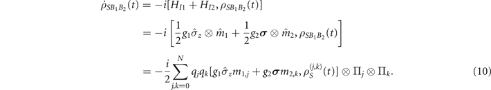
Owing to [H_S , H_I1 + H_I2] = 0, the differential equation corresponding to the density matrix of the total system can be obtained by using the global von Neumann equation in the interaction picture:

$$\begin{align}{\dot{\rho }}_{S{B}_{1}{B}_{2}}(t)& =-i[{H}_{I1}+{H}_{I2},{\rho }_{S{B}_{1}{B}_{2}}(t)]\\ & =-i\left[\frac{1}{2}{g}_{1}{\hat{\sigma }}_{z}\otimes {\hat{m}}_{1}+\frac{1}{2}{g}_{2}\boldsymbol{\sigma }\otimes {\hat{m}}_{2},{\rho }_{S{B}_{1}{B}_{2}}(t)\right]\\ & =-\frac{i}{2}\sum\limits _{j,k=0}^{N}{q}_{j}{q}_{k}[{g}_{1}{\hat{\sigma }}_{z}{m}_{1,j}+{g}_{2}\boldsymbol{\sigma }{m}_{2,k},{\rho }_{S}^{(j,k)}(t)]\otimes {{\Pi}}_{j}\otimes {{\Pi}}_{k}.\end{align} \tag{ 10 }$$

As no coupling occurs between different magnetization subspaces in our model, each of the conditional states ${\rho }_{S}^{(j,k)}(t)$ in equation (10) evolves independently. Therefore, we can obtain a set of uncoupled differential equations for each conditional state, as follows:

$$\begin{equation}{\dot{\rho }}_{S}^{(j,k)}(t)=-\frac{i}{2}[{g}_{1}{\hat{\sigma }}_{z}{m}_{1,j}+{g}_{2}\boldsymbol{\sigma }{m}_{2,k},{\rho }_{S}^{(j,k)}(t)].\end{equation} \tag{ 11 }$$

Subsequently, the above spin system dynamics can be rewritten in the Bloch sphere representation ${\rho }_{S}=\frac{1}{2}(\mathbb{I}+\mathbf{r}\cdot \boldsymbol{\sigma })$, where the Bloch vector r unambiguously specifies the state of the system, $\mathbf{r}=({r}_{x},{r}_{y},{r}_{z})\in B{:=}\left\{\mathbf{r}\in {\mathfrak{R}}^{3};{\Vert}\mathbf{r}{\Vert}\leqslant 1\right\}$, and $\mathbb{I}$ is the identity operator of the system. Therefore, equation (11) can be expressed as follows:

$$\begin{equation}{\dot{\mathbf{r}}}^{(j,k)}(t)\cdot \boldsymbol{\sigma }=-\frac{i}{2}[{g}_{1}{\hat{\sigma }}_{z}{m}_{1,j}+{g}_{2}\boldsymbol{\sigma }{m}_{2,k},{\mathbf{r}}^{(j,k)}(t)\cdot \boldsymbol{\sigma }],\end{equation} \tag{ 12 }$$

and

$$\begin{equation}\mathbf{r}(t)={\mathbf{D}}_{t}\mathbf{r}(0)=\left[\sum\limits _{j,k}\;p({m}_{1,j})p({m}_{2,k}){\mathbf{R}}_{12}^{(j,k)}(t)\right]\mathbf{r}(0).\end{equation} \tag{ 13 }$$

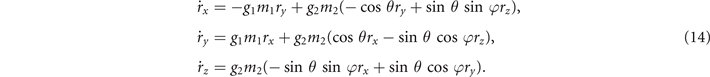
On the Cartesian basis, we drop the indices j, k and ignore the explicit time dependence for simplicity. Subsequently, equation (12) can be expanded into the following differential equations:

$$\begin{equation}\begin{aligned}{\dot{r}}_{x}& =-{g}_{1}{m}_{1}{r}_{y}+{g}_{2}{m}_{2}(-\mathrm{cos}\enspace \theta {r}_{y}+\mathrm{sin}\enspace \theta \enspace \mathrm{sin}\enspace \varphi {r}_{z}),\\ {\dot{r}}_{y}& ={g}_{1}{m}_{1}{r}_{x}+{g}_{2}{m}_{2}(\mathrm{cos}\enspace \theta {r}_{x}-\mathrm{sin}\enspace \theta \enspace \mathrm{cos}\enspace \varphi {r}_{z}),\\ {\dot{r}}_{z}& ={g}_{2}{m}_{2}(-\mathrm{sin}\enspace \theta \enspace \mathrm{sin}\enspace \varphi {r}_{x}+\mathrm{sin}\enspace \theta \enspace \mathrm{cos}\enspace \varphi {r}_{y}).\end{aligned}\end{equation} \tag{ 14 }$$

In the limit of N → ∞, the affine transformation can be performed in the following manner:

$$\begin{equation}{\mathbf{D}}_{t}=\sum\limits _{j,k}\;p({m}_{1,j})p({m}_{2,k}){\mathbf{R}}_{12}^{(j,k)}(t)\underset{N\to \infty }{\to }{\int }_{-\infty }^{\infty }{\int }_{-\infty }^{\infty }\mathrm{d}{m}_{1}\enspace \mathrm{d}{m}_{2}\enspace p({m}_{1})p({m}_{2}){\mathbf{R}}_{12}({m}_{1},{m}_{2},t),\end{equation} \tag{ 15 }$$

where R₁₂(m₁, m₂, t), which possesses two magnetization parameters that are associated with each magnet, can be analytically acquired from equation (14). Hence, the Bloch vector r(t) of the density matrix at any time can be obtained from any initial state r(0).

By applying a static Zeeman field to drive a spin-1/2 system S, we mainly focus on the dynamics of the spin system coupled with a magnet B, as depicted in figure 1. Similar to model A, the magnetic environment follows a Gaussian distribution, and the free Hamiltonian of the magnet is selected as H_B = 0. The Hamiltonian of the spin system that is affected by the static Zeeman field is as follows [62]:

$$\begin{equation}{H}_{S}=\frac{1}{2}\omega {\boldsymbol{\sigma }}_{0}^{(n)},\end{equation} \tag{ 16 }$$

where ω behaves as the static Zeeman field and the component ${\boldsymbol{\sigma }}_{0}^{(n)}$ of the spin system can be selected as σ_x , σ_y , or σ_z . The interaction Hamiltonian between the spin system and magnet is expressed as

$$\begin{equation}{H}_{I}=\frac{1}{2}g{\boldsymbol{\sigma }}_{1}^{(n)}\otimes \hat{m},\end{equation} \tag{ 17 }$$

where the coupling strength between the system and magnet is g, and the coupling component of the spin system to the magnet is ${\boldsymbol{\sigma }}_{1}^{(n)}$, which can also be selected as σ_x , σ_y , or σ_z . Furthermore, ${\boldsymbol{\sigma }}_{0}^{(n)}$ and ${\boldsymbol{\sigma }}_{1}^{(n)}$ should be selected for a set of Pauli matrices that are not commutative with one another, $[{\boldsymbol{\sigma }}_{0}^{(n)},{\boldsymbol{\sigma }}_{1}^{(n)}]\ne 0$; that is, corresponding to the case of [H_S , H_I ] ≠ 0. Therefore, to solve the open system dynamics precisely by using the same calculation method as that of model A, we first need to compute the interaction Hamiltonian in the interaction picture:

$$\begin{equation}\bar{{H}_{I}}={e}^{\frac{i}{2}\omega {\boldsymbol{\sigma }}_{0}^{(n)}t}{H}_{I}{e}^{\frac{-i}{2}\omega {\boldsymbol{\sigma }}_{0}^{(n)}t}.\end{equation} \tag{ 18 }$$

The initial state of the total system is considered as ρ_SB (0) = ρ_S (0) ⊗ ρ_B , where the initial state of the magnetic environment is also selected as a classical mixture of different magnetizations ${\rho }_{B}={\sum }_{k=0}^{N}\;{q}_{k}{{\Pi}}_{k}$, in which q_k  Tr[Π_k ] = Tr[ρ_B Π_k ] = p(m_k ) represents the initial probability that the observations of the magnetizations will yield m_k . Analogously to model A, using the global von Neumann equation, the Bloch vector ${\bar{\mathbf{r}}}^{(k)}(t)={e}^{\frac{-i}{2}\omega {\boldsymbol{\sigma }}_{0}^{(n)}t}{\mathbf{r}}^{(k)}(t)$ in the interaction picture represents the spin system state that is conditioned on the magnet possessing magnetization m_k :

$$\begin{equation}{\dot{\bar{\mathbf{r}}}}^{(k)}(t)\cdot \boldsymbol{\sigma }=-i[\bar{{H}_{I}},{\bar{\mathbf{r}}}^{(k)}(t)\cdot \boldsymbol{\sigma }].\end{equation} \tag{ 19 }$$

To obtain the solution of the differential equations, the homomorphism transformation of the SU₂ group and SO₃ group should be used by converting the unitary transformation element ${e}^{\frac{i}{2}\omega {\boldsymbol{\sigma }}_{0}^{(n)}t}$ into ${\mathbf{R}}_{U}^{(n)}(t)$. In this case, ${\mathbf{R}}_{U}^{(n)}(t)$ can be expressed in varying forms for the different ${\boldsymbol{\sigma }}_{0}^{(n)}$ (n = x, y, or z):

$$\begin{equation}{\mathbf{R}}_{U}^{(x)}(t)\equiv \left(\begin{matrix}\hfill 1\hfill & \hfill 0\hfill & \hfill 0\hfill \\ \hfill 0\hfill & \hfill \mathrm{cos}(\omega t)\hfill & \hfill -\mathrm{sin}(\omega t)\hfill \\ \hfill 0\hfill & \hfill \mathrm{sin}(\omega t)\hfill & \hfill \mathrm{cos}(\omega t)\hfill \end{matrix}\right),\end{equation} \tag{ 20 }$$

$$\begin{equation}{\mathbf{R}}_{U}^{(y)}(t)\equiv \left(\begin{matrix}\hfill \mathrm{cos}(\omega t)\hfill & \hfill 0\hfill & \hfill \mathrm{sin}(\omega t)\hfill \\ \hfill 0\hfill & \hfill 1\hfill & \hfill 0\hfill \\ \hfill -\mathrm{sin}(\omega t)\hfill & \hfill 0\hfill & \hfill \mathrm{cos}(\omega t)\hfill \end{matrix}\right),\end{equation} \tag{ 21 }$$

$$\begin{equation}{\mathbf{R}}_{U}^{(z)}(t)\equiv \left(\begin{matrix}\hfill \mathrm{cos}(\omega t)\hfill & \hfill -\mathrm{sin}(\omega t)\hfill & \hfill 0\hfill \\ \hfill \mathrm{sin}(\omega t)\hfill & \hfill \mathrm{cos}(\omega t)\hfill & \hfill 0\hfill \\ \hfill 0\hfill & \hfill 0\hfill & \hfill 1\hfill \end{matrix}\right).\end{equation} \tag{ 22 }$$

The differential equations proceed as follows:

$$\begin{equation}{\dot{\tilde{\mathbf{r}}}}^{(k)}(t)={\mathbf{R}}_{U}^{(n)}(t)\cdot {\mathbf{Q}}^{(n)}\cdot {\dot{\bar{\mathbf{r}}}}^{(k)}(t),\end{equation} \tag{ 23 }$$

where Q⁽ⁿ⁾ is also determined according to the different ${\boldsymbol{\sigma }}_{0}^{(n)}$ (n = x, y, or z):

$$\begin{equation}{\mathbf{Q}}^{(x)}\equiv \mathrm{diag}\left\{1,-1,1\right\},\end{equation} \tag{ 24 }$$

$$\begin{equation}{\mathbf{Q}}^{(y)}\equiv \mathrm{diag}\left\{1,1,-1\right\},\end{equation} \tag{ 25 }$$

$$\begin{equation}{\mathbf{Q}}^{(z)}\equiv \mathrm{diag}\left\{-1,1,1\right\}.\end{equation} \tag{ 26 }$$

Following the above rotation operation Q⁽ⁿ⁾, the matrix $\tilde{\mathbf{R}}(m,t)$ can be obtained, which contains the influence of the magnet. At this point, the differential equations of the above system become solvable. Subsequently, the solved matrix $\tilde{\mathbf{R}}(m,t)$ can be converted back into the interaction scenario:

$$\begin{equation}\bar{\mathbf{R}}(m,t)={({\mathbf{R}}_{U}^{(n)}(t)\cdot {\mathbf{Q}}^{(n)})}^{-1}\tilde{\mathbf{R}}(m,t)({\mathbf{R}}_{U}^{(n)}(t)\cdot {\mathbf{Q}}^{(n)}).\end{equation} \tag{ 27 }$$

In the limit of N → ∞, we can obtain ${\bar{\mathbf{D}}}_{t}$ for this model:

$$\begin{equation}{\bar{\mathbf{D}}}_{t}={\int }_{-\infty }^{\infty }\mathrm{d}m\enspace p(m)\bar{\mathbf{R}}(m,t).\end{equation} \tag{ 28 }$$

Thereafter, by substituting the result into $\bar{\mathbf{r}}(t)={\bar{\mathbf{D}}}_{t}\bar{\mathbf{r}}(0)$, the evolution-reduced density matrix of the spin system that is affected by a static Zeeman field can be obtained.

In the following, we set the initial state of the system to the maximal coherent state r(0) = (±1, 0, 0) for the above two models. Subsequently, we mainly analyze the control of the non-Markovian dynamics behavior of the spin system in the magnets under the above models.

Based on the original spin-magnet model, we add a new second magnet to affect the dynamics of the spin-1/2 system. The interaction Hamiltonians are provided by equations (4) and (5). By setting the initial state of the qubit to the maximal coherent states (the optimal state pair to calculate the non-Markovianity) r_x = ±1, r_y = r_z = 0, we demonstrate how to manipulate the non-Markovianity of the open dynamics process under model A by adjusting two coupling direction angles (θ and φ) of the spin system to the new magnet, and the magnetic-related parameters (such as the standard deviations of the Gaussian distribution of two independent magnets).

First, for the spin system that is simultaneously coupled to two magnetic environments with the same components ($\boldsymbol{\sigma }={\hat{\sigma }}_{z}$; that is, [H_I1, H_I2] = 0), figure 2 indicates that the distinguishability between the two states described by the trace distance $D({\rho }_{1}^{S}(\tau ),{\rho }_{2}^{S}(\tau ))$ monotonically decreases with time by considering the different coupling strengths g₂/g₁ between the spin and two magnets. Thus, the non-Markvoianity of the dynamics process of the system is always zero, regardless of how the magnetic environments are controlled. This indicates that the Markovian dynamics of the system cannot be transformed into the non-Markovian process when the interaction Hamiltonians commute with one another. This result is the same as that of the system dynamics in the original spin-magnet model. The main reason for this is that, when [H_I1, H_I2] = 0, the system dynamics can be naively solved by adding the generators in equation (3).

Zoom In Zoom Out Reset image size

Hence, for the purpose of obtaining the non-Markovian behavior of the dynamics process in model A, we investigate how to manipulate the non-Markovianity of the dynamics process in the case of the spin system that simultaneously interacts with two magnets by means of two different spin components $[{\hat{\sigma }}_{z},\boldsymbol{\sigma }]\ne 0$; that is, the two interaction Hamiltonians do not commute with one another: [H_I1, H_I2] ≠ 0. Considering the two same magnets (λ₁ = λ₂), and the spin component $\mathrm{cos}\enspace \varphi {\hat{\sigma }}_{x}+\mathrm{sin}\enspace \varphi {\hat{\sigma }}_{y}$ of the second magnet, the non-Markovianity of the dynamics process from the initial state ρ(0) to the final target state ρ(τ) is presented in figure 3, where the parameters satisfy θ = π/2. We can explicitly determine that the original Markovian dynamics behavior (N_BLP = 0) can be transformed into the new non-Markovian dynamics behavior (N_BLP > 0) by introducing a second magnet that is coupled with the spin system, as indicated by the colored region in figure 3(b). This result is mainly because dynamics behavior corresponding to a system that simultaneously interacts with two magnets with two noncommutative interaction Hamiltonians cannot be constructed by the simple addition of the dynamics behavior associated with each individual environment. The cross-correlation that nay emerge between the two environments owing to their noncommutative interactions with the system leads to the new non-Markovian dynamics behavior.

Zoom In Zoom Out Reset image size

According to figure 3, the effects of the direction angle φ (which implies the different spin components of the spin system of the second magnet) on the non-Markovianity of the open dynamics process can be investigated further. A remarkable behavior of the sudden transition from N_BLP = 0 to N_BLP > 0 is dependent on the selection of the final target state ρ(τ). There exists a critical evolution target state ρ(τ_c). In the case of the dynamics process with the actual evolution time τ < τ_c, the information backflow from the magnetic environments to the spin system never occurs, regardless of the selected value of φ. However, in the case of τ > τ_c, the information backflow always occurs based on the selection of an appropriate φ for coupling the component of the spin system to the second magnet. This means that the non-Markovian dynamics behavior of the dynamics process from ρ(0) to ρ(τ) (τ > τ_c) can be controlled by adding the second magnet that is coupled to the spin system.

Again, for a given dynamics process, such as the actual evolution dimensionless time τ = 4, it is worth noting that the non-Markovianity of the evolution will first gradually decrease and then gradually increase with an increase in φ in the region [0, π/2], as shown in figure 3(a). Moreover, when the interaction Hamiltonian between the spin system and added second magnetic environment satisfies $\frac{1}{2}{g}_{2}{\hat{\sigma }}_{y}\otimes {\hat{m}}_{2}$ (corresponding to φ = π/2), the maximum non-Markovianity of the dynamics process can be acquired. Therefore, according to the above analysis, we obtain the interesting result that when the spin system is coupled to two independent magnets with two noncommutative interaction Hamiltonians, the new non-Markovian dynamics behavior of the spin can be achieved. Furthermore, in the case of a measurement of the component ${\hat{\sigma }}_{z}$ of the spin system by the first magnet, the maximum non-Markovianity of the dynamics process can be acquired by simultaneously measuring the component ${\hat{\sigma }}_{y}$ of the spin system by the second magnet, as illustrated in figure 3(a). However, when H_I2 contains the two different spin components of the system (${\hat{\sigma }}_{x}$ and ${\hat{\sigma }}_{y}$) of the second magnet, it is clear that when the weights of the operators ${\hat{\sigma }}_{x}\otimes {\hat{m}}_{2}$ and ${\hat{\sigma }}_{y}\otimes {\hat{m}}_{2}$ are closer (φ around π/4), the non-Markovianity of the dynamics process is reduced. A potential 'counteracting' effect exists in the production of the non-Markovian behavior of the dynamics process.

In the spin-magnet model, the standard deviation in the Gaussian distribution of the magnet and the coupling strength between the magnet and system are parameters that can be easily controlled. Thus, in the following, according to the case in which the spin system is coupled to two magnets with different components (${\hat{\sigma }}_{z}\otimes {\hat{m}}_{1}$ and ${\hat{\sigma }}_{y}\otimes {\hat{m}}_{2}$), for the given coupling strength g₁ between the spin system and first magnet with a standard deviation λ₁ of the Gaussian distribution, we analyze the effects of the coupling strength of the system with the second magnet g₂ and the standard deviation of the Gaussian distribution of this magnet λ₂ on the non-Markovianity of the dynamics process, as illustrated in figure 4(a). We can explicitly conclude that the non-Markovianity first increases and then decreases with an increase in λ₂. Furthermore, the maximum non-Markovianity of the dynamics process (ρ(0) to ρ(τ = 2)) is strongly dependent on the related parameters of the second magnet (g₂ and λ₂). The numerical calculation also demonstrates that the optimal value of the standard deviation of the Gaussian distribution of this magnet ${\lambda }_{2}^{\text{opt}}$ is determined by the coupling strength of the system to the second magnet g₂. A smaller value of g₂ results in a larger optimal value of ${\lambda }_{2}^{\text{opt}}$ that should be requested. Taking the cases in figure 4(a) as examples, when g₂ = 0.3g₁, the optimal value of the standard deviation of the Gaussian distribution of this magnet is ${\lambda }_{2}^{\text{opt}}=3.6{\lambda }_{1}$. In the cases of g₂ = g₁ and g₂ = 3g₁, we can obtain ${\lambda }_{2}^{\text{opt}}=1.1{\lambda }_{1}$ and ${\lambda }_{2}^{\text{opt}}=0.4{\lambda }_{1}$, respectively.

Zoom In Zoom Out Reset image size

In recent years, it has been determined that the non-Markovianity of the dynamics process can be attributed to the quantum speedup of the evolution of a quantum system [31]. However, the question remains whether the one-to-one relationship between the non-Markovianity and quantum speedup holds true. Figure 4(b) describes the effects of the adjustable related parameters (g₂ and λ₂) of the second magnet on the QSLT of the spin system. It can clearly be observed that, as λ₂ increases, the value of τ_qsl/τ can transition from τ_qsl/τ = 1 to τ_qsl/τ < 1, and then to τ_qsl/τ = 1. Similar to the analysis of the maximum non-Markovianity of the dynamics process (ρ(0) to ρ(τ = 2)), the optimal value of λ₂ for the minimum τ_qsl/τ (which means the maximal quantum evolution speed) of this dynamics process is determined by the coupling strength of the system to the second magnet g₂. As indicated in figure 4(b), a smaller value of g₂ results in a larger optimal value of λ₂ that should be requested. Thereafter, speedup evolution of the spin system can occur by selecting the suitable parameter region of λ₂.

However, as opposed to the situation of previous studies, the QSLT is not strictly correlated with the occurrence of the non-Markovianity of the dynamics process, as illustrated in figure 4. Unexpectedly, non-Markovianity of the studied dynamics process exists, whereas the evolution speed of this dynamics process will not be accelerated, as indicated by the blue dotted lines in figures 4(a) and (b). Although the non-Markovianity may play an active role in the QSLT, the quantum speedup of the dynamics process is not only affected by the non-Markovianity. The geometric distance ${{\Vert}\rho \left(\tau \right)-\rho \left(0\right){\Vert}}_{hs}$ between the initial state ρ(0) and final target state ρ(τ) may also be an important factor affecting the QSLT.

In the above subsection, it was explained that the non-Markovian dynamics behavior can be obtained by controlling the newly added magnet for the spin-1/2 system. At this point, we propose the other scheme for manipulating the non-Markovian dynamics behavior by applying a static Zeeman field on the spin-1/2 system. The spin system Hamiltonian H_S that is affected by the Zeeman field and the interaction Hamiltonian H_I are expressed as $\frac{1}{2}\omega {\boldsymbol{\sigma }}_{0}^{(n)}$ and $\frac{1}{2}g{\boldsymbol{\sigma }}_{1}^{(n)}\otimes \hat{m}$, respectively. By setting the initial state of the spin system to the maximal coherent state (the optimal state pair to calculate the non-Markovianity) r_x = ±1, r_y = r_z = 0, the dynamics of the system can be calculated using the method outlined in section 2.

According to the different combinations of H_S and H_I in model B (labeled as (${\boldsymbol{\sigma }}_{0}^{(n)}$, ${\boldsymbol{\sigma }}_{1}^{(n)}$)), for a given dynamics process from the initial state ρ(0) to the final target state ρ(τ), the non-Markovianity and the QSLT for this dynamics process are calculated, as displayed in table 1. First, it can be clearly observed that the non-Markovian dynamics behavior and corresponding speedup dynamics of the evolution process never arise in the case of ${\boldsymbol{\sigma }}_{0}^{(n)}={\boldsymbol{\sigma }}_{1}^{(n)}$, which means that [H_S , H_I ] = 0. However, according to table 1, in the case of the non-commutative relationship [H_S , H_I ] ≠ 0, the non-Markovian dynamics behavior and corresponding speedup dynamics of the evolution process can be acquired in the remaining six combinations of H_S and H_I , namely (σ_x , σ_y ), (σ_x , σ_z ), (σ_y , σ_x ), (σ_y , σ_z ), (σ_z , σ_x ), and (σ_z , σ_y ). Interestingly, the same values of the non-Markovianity and QSLT for a given dynamics process can be obtained by the different combinations of the static Zeeman field of the spin component and the coupling of the spin component to the magnet (${\boldsymbol{\sigma }}_{0}^{(n)}$, ${\boldsymbol{\sigma }}_{1}^{(n)}$); that is (i) (${\hat{\sigma }}_{y}$, ${\hat{\sigma }}_{z}$) and (${\hat{\sigma }}_{z}$, ${\hat{\sigma }}_{y}$), (ii) (${\hat{\sigma }}_{x}$, ${\hat{\sigma }}_{z}$) and (${\hat{\sigma }}_{x}$, ${\hat{\sigma }}_{y}$), and (iii) (${\hat{\sigma }}_{z}$, ${\hat{\sigma }}_{x}$) and (${\hat{\sigma }}_{y}$, ${\hat{\sigma }}_{x}$).

Table 1. Non-Markovianity and QSLT under different combinations of H_S and H_I , with g = 1.

${\boldsymbol{\sigma }}_{0}^{(n)}$	${\boldsymbol{\sigma }}_{1}^{(n)}$	τ	ω	λ	NBLP	τqsl/τ
σx	σx	10	1	1	0	1
		10	1	2	0	1
		10	2	1	0	1
σx	σy	10	1	1	0.419 574	0.274 127
		10	1	2	0.352 056	0.438 436
		10	2	1	0.437 348	0.170 007
σx	σz	10	1	1	0.419 574	0.274 127
		10	1	2	0.352 056	0.438 436
		10	2	1	0.437 348	0.170 007
σy	σx	10	1	1	0.933 145	0.321 245
		10	1	2	0.642 920	0.251 091
		10	2	1	0.741 944	0.190 870
σy	σy	10	1	1	0	1
		10	1	2	0	1
		10	2	1	0	1
σy	σz	10	1	1	0.043 377	0.697 160
		10	1	2	0.019 902	0.720 427
		10	2	1	0.059 210	0.684 268
σz	σx	10	1	1	0.933 145	0.321 245
		10	1	2	0.642 920	0.251 091
		10	2	1	0.741 944	0.190 870
σz	σy	10	1	1	0.043 377	0.697 160
		10	1	2	0.019 902	0.720 427
		10	2	1	0.059 210	0.684 268
σz	σz	10	1	1	0	1
		10	1	2	0	1
		10	2	1	0	1

To investigate the effects of the different operation combinations in model B on the non-Markovianity of the dynamics process from ρ(0) to ρ(τ) further, figure 5 presents the phase diagram of the non-Markovianity under three different operation combinations (${\hat{\sigma }}_{y}$, ${\hat{\sigma }}_{z}$), (${\hat{\sigma }}_{x}$, ${\hat{\sigma }}_{z}$), and (${\hat{\sigma }}_{z}$, ${\hat{\sigma }}_{x}$). It can easily be observed that all these three operation combinations in model B can transform the original Markovian behavior into non-Markovian behavior when the appropriate parameters (ω and λ) are selected. The non-Markovianity is the weakest in case (i), whereas it is the strongest in case (iii). Thus, to acquire substantially greater non-Markovianity of the dynamics process, a static Zeeman field can be used along the ${\hat{\sigma }}_{z}$ (or ${\hat{\sigma }}_{y}$) component of the spin system, which couples to the magnet in the ${\hat{\sigma }}_{x}$ component.

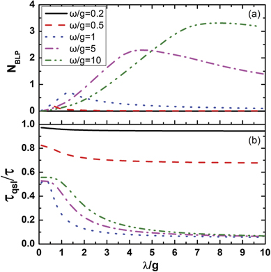
Zoom In Zoom Out Reset image size

Moreover, the static Zeeman field ω and standard deviation of the Gaussian distribution of the magnet λ are crucial to the appearance of non-Markovian behavior. Using the optimal operation combination (${\hat{\sigma }}_{z}$, ${\hat{\sigma }}_{x}$) as an example, the non-Markovianity and QSLT of a given dynamics process from ρ(0) to ρ(τ = 6) are calculated as illustrated in figure 6. Therefore, by considering the different static Zeeman fields ω, we reach the interesting result that the non-Markovianity first increases and then decreases with an increase in the standard deviation λ of the magnet. Furthermore, there exists an optimal λ^opt that corresponds to the non-Markovianity maximum of the dynamics process. The optimal λ^opt and non-Markovianity maximum are strongly dependent on the static Zeeman field ω. A larger value of ω results in a larger optimal value of λ^opt that should be requested to acquire the larger non-Markovianity maximum, as illustrated in figure 6(a). Again, in the case of the weak static Zeeman field (such as the cases of ω/g = 0.2 and ω/g = 0.5 in figure 6(a)), it must be emphasized that the evolution of the spin system abides by the Markovian dynamics behavior and is hardly affected by the standard deviation of the Gaussian distribution of the magnet.

Zoom In Zoom Out Reset image size

Moreover, as indicated in figure 6(b), τ_qsl/τ is always less than 1, and it decreases with the increase in the standard deviation λ of the magnet, regardless of the value of ω. Therefore, in the model in which a static Zeeman field is applied on the spin system, the system evolution is always accelerated. Furthermore, according to figure 6(b), the intermediate value of the static Zeeman field ω has an impact on the smaller τ_qsl/τ, as indicated by the blue dotted line (ω/g = 1), whereas the non-Markovianity of this dynamics process is not larger. Compared to the previous analysis of the non-Markovianity, the stronger non-Markovianity does not lead to greater quantum acceleration. This again clearly demonstrates that there is no direct relationship between the non-Markovianity and quantum speedup of the dynamics process of the open system.