


Abstract
Decades of agricultural intensification have led to elevated stream nitrogen (N) concentrations and eutrophication of inland and coastal waters. Despite widespread implementation of a range of strategies to reduce N export, expected improvements in water quality have not been observed. This lack of success has often been attributed to the existence of legacy N stores within the landscape. Here, we use the ELEMeNT-N model to quantify legacy accumulation and depletion dynamics over the last century (1930–2016) across 14 nested basins within the Grand River Watershed, a 6800 km2 agricultural watershed in the Lake Erie Basin. Model results reveal significant legacy N accumulation across the basin, ranging from 705 to 1071 kg ha−1, creating a checkered landscape of N legacies. The largest proportion (82%–96%) of this accumulated N is stored in soil organic N reservoirs, as biogeochemical legacy, and the remaining in groundwater, as hydrologic legacy. The fraction of N surplus accumulated in soil and groundwater is most strongly correlated with the calibrated watershed mean travel time µ, with the accumulation increasing with increases in µ. The mean travel time ranges from 5 to 34 years across the watersheds studied, and increases with increase in tile drainage, highlighting the strong control of anthropogenic management on legacy accumulation. Water quality improvement timescales were found to be heterogeneous across the watersheds, with greater legacies contributing to slower recovery.
Export citation and abstract BibTeX RIS

Original content from this work may be used under the terms of the Creative Commons Attribution 4.0 license. Any further distribution of this work must maintain attribution to the author(s) and the title of the work, journal citation and DOI.
1. Introduction
Global population has increased more than threefold over the last 100 years, accompanied by agricultural intensification and rapid changes in land use. Such changes have been accompanied by a great acceleration of the nitrogen (N) cycle, with exponential increases in the use of commercial fertilizers since 1900. Excess N from agricultural activities leaches to both surface and groundwater, leading to problems of eutrophication, aquatic toxicity and drinking water contamination (Carpenter et al 1998, Di and Cameron 2002, Howarth et al 2002, Dodds 2006, Heisler et al 2008, Kleinman et al 2011, Mekonnen and Hoekstra 2018, Tornqvist et al 2015, Van Meter et al 2020). An increased occurrence of harmful algal blooms and hypoxia has been documented all over the world, including, the Gulf of Mexico in North America (Turner et al 2008), lakes and coastal waters in Denmark (Kronvang et al 2005), and Lake Erie in North America (Watson et al 2016).
Over the last 50 years, efforts have been made to reduce N discharges using a range of approaches, including upgrades in performance of wastewater treatment plants (WWTPs), atmospheric emission reduction policies (Lloret and Valiela 2016, Maccoux et al 2016), and implementation of various agricultural best management practices (BMPs) (Mitchell and Shrubsole 1992, Kaika 2003, International Joint Commission 2005, Zbieranowski and Aherne 2011, Liu et al 2017). Despite these efforts, targets for water quality improvement have generally not been met (Carpenter et al 1998, Sharpley et al 2009, Worrall et al 2009, Sprague and Gronberg 2012, Liu et al 2017, Choquette et al 2019, Van Meter et al 2018, Van Meter et al 2019). For example, there have been extensive efforts in the Mississippi and the Chesapeake Bay to reduce N loading for more than 20 years by widespread implementation of BMPs, but neither have reached their target loads (Van Meter et al 2018, Chang et al 2021). In Europe, only 31% of designated Nitrate Vulnerable Zones have seen improvements in water quality, while many areas have experienced increased nitrate loadings (Worrall et al 2009).
One of the reasons behind such apparent lack of success lies in the existence of N legacies within the landscape that have built up over decades of agricultural intensification (Hamilton 2012, Van Meter and Basu 2017, Basu et al 2010, Van Meter et al 2016, Thompson et al 2011) and can contribute to elevated nutrient concentrations for multiple years after inputs have decreased. Such time lags have been found to range from 5 to more than 50 years (Meals et al 2010, Vero et al 2017). While the scientific community is increasingly aware of the existence of nitrogen legacies, we still lack tools and methodologies to quantify legacies and time lags for policy and decision-making (Meals et al 2010, Van Meter et al 2016, Chen et al 2018). For nitrogen, it has been shown that legacies can accumulate as organic N in the root zone of agricultural soils (biogeochemical legacy), or as dissolved nitrate in groundwater and soil water (hydrologic legacy) (Hamilton 2012, Van Meter and Basu 2017, Van Meter et al 2016) However, quantification of the magnitudes of such accumulation based on direct monitoring is often difficult due to spatial heterogeneity within the landscape (Bouraoui and Grizzetti 2014, Chen et al 2018).
Models can potentially fill this gap; however, most available water quality models, including the Soil Water Assessment tool (SWAT), Geospatial Regression for European Nutrient Losses, and Modelling Nutrient Emissions in River Systems, do not explicitly consider legacies and time lags (Bouraoui and Grizzetti 2014, Van Meter et al 2017, Shafii et al 2019). While some empirical models have been adapted to account for lag times, the lack of process conceptualizations makes it impossible to detangle the legacy accumulated in various landscape elements (Behrendt et al 2000, Hong et al 2017, Van Meter and Basu 2017, Chen et al 2018). The process-based model, SWAT, has recently been adapted for modelling nutrient lag times, but its complexity when accounting for changing land use may be overly restrictive for wide adoption (Chen et al 2018, Ilampooranan et al 2019). The ELEMeNT-N (Exploration of Long-Term Nutrient Trajectories for Nitrogen) model was the first process-based approach to quantify nitrogen legacies and lag times at the watershed and the regional scale (Van Meter et al 2017, 2018, 2019). The model has now been applied to two large basins in the US, the Mississippi River Basin (MRB) and the Chesapeake Bay Watershed (CPB) (Van Meter et al 2017, 2018, Chang et al 2021) to estimate nitrogen legacies and lag times. We found contrasting results in the two watersheds, with the CPB results suggesting that goals to reduce N loads can be met in the next two decades even without any changes in management practices (Chang et al 2021). In contrast, results in the MRB suggest that even with a 100% reduction in N surplus, it would take over 30 years to meet the N reduction goals recommended by the Hypoxia Task force (Van Meter et al 2018). These studies highlight the heterogeneity in responses across watersheds, and underscore the need to understand how legacy accumulation and depletion vary as a function of landscape and management controls in different landscapes.
Knowledge is also lacking regarding how legacy N accumulation may vary along a river network, and the landscape attributes that control spatial patterns of legacy accumulation. This is important for designing appropriate watershed management strategies that target hotspots in legacy accumulation to achieve the fastest and largest improvements in water quality. The overall goal of this paper is to address this knowledge gap. We use as a case study the Grand River Watershed (GRW), a 6800 km2 agricultural watershed draining into the eastern basin of Lake Erie, and address the following questions: (a) How have N inputs and non-hydrologic outputs (crop uptake) changed over the last century across the GRW? (b) How do N stores (soil and groundwater reservoirs), and fluxes (stream export, denitrification) vary across nested subbasins within the GRW? (c) What are the landscape and management controls on legacy accumulation? (d) How do the accumulated N legacies contribute to time lags in achieving N export reduction goals?
2. ELEMeNT-N modelling framework
The ELEMeNT-N model utilizes a coupled framework that links source-zone dynamics, describing the accumulation and depletion of soil organic nitrogen (SON) within the root zone, with a travel time model that describes transport and transformations along hydrologic pathways to the stream outlet (figure S1 available online at stacks.iop.org/ERL/16/115006/mmedia). ELEMeNT-N conceptualizes the landscape as a bundle of stream-tubes, each with a unique travel time to the watershed outlet such that the landscape as a whole can be characterized by the travel time distribution f(τ) (McGuire and McDonnell 2006, Van Meter et al
2017, Basu et al
2012, Van Meter et al
2015) that controls the flux of nitrogen  [ML−2 T−1] at the watershed outlet:
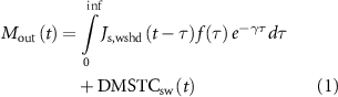
where Js,wshd (t) [ML−2 T−1] is the source function, which describes the flux of nitrate-N from the source zone to the subsurface pathways; f(τ) describes the landscape travel time distribution that we have assumed to be exponential (f(τ) =  ; where τ [T] is the travel time and µ [T] is the mean travel time); γ [T−1] is the first-order rate constant that describes N removal via denitrification along hydrologic pathways (Basu et al
2011);
; where τ [T] is the travel time and µ [T] is the mean travel time); γ [T−1] is the first-order rate constant that describes N removal via denitrification along hydrologic pathways (Basu et al
2011);  [ML−2 T−1] is wastewater-N discharge to the stream, which is a function of the population density, and a retention rate constant kh [T−1] that captures both denitrification and removal in biosolids in the WWTPs (Van Meter et al
2017) (supplementary SI 1.0).
[ML−2 T−1] is wastewater-N discharge to the stream, which is a function of the population density, and a retention rate constant kh [T−1] that captures both denitrification and removal in biosolids in the WWTPs (Van Meter et al
2017) (supplementary SI 1.0).
The critical element that distinguishes ELEMeNT from other watershed models is that it explicitly considers not only the effects of current-year N inputs to the landscape, but also the role of past land use and land management and legacy N stores on stream N fluxes (Van Meter et al 2017). Accordingly, the watershed is divided into s distinct units, each assigned a unique land-use trajectory, and the temporal evolution of the trajectories is stored within a 2D land use array, LU(s, t),
where Acrop (t) and Apast (t) are the watershed percent cropland and pastureland areas, respectively.
The source function Js,wshd (t) is estimated as a function of the N surplus to the soil surface (equations (3)–(5)), and soil hydrological and biogeochemical factors, including the SON content in pristine soils (Ms [ML−2]), denitrification rate constants is soil and groundwater (λs and λ [T−1]), mineralization rate constants (ka [T−1]) and humification coefficients (hnc and hc) (SI section 1.1.4 and table S2). We estimated the N surplus on cropland, pastureland and non-agricultural land using a surface N balance approach (Bouwman et al 2005, Byrnes et al 2020) across the different landscape types, with surplus N being defined as the difference between landscape N inputs (livestock manure, mineral N fertilizer, biological nitrogen fixation, and atmospheric N deposition) and N uptake (Leip et al 2011):
where,  ,
,  , and
, and  is the N surplus applied to cropland, pastureland, or non-agricultural land at the soil surface;
  and
and  refer to inorganic N fertilizer;
  represents livestock manure N applied to cropland;
  represents both manure N applied to pastureland as well as livestock N excretion during grazing;
  refers to atmospheric N deposition;
  ,
,  and
and  refers to biological N fixation on cropland, pastureland and non-agricultural land;
  ,
,  and
and  represents N removal by crop uptake, livestock grazing and forest uptake, respectively. All fluxes in equations (3)–(5) are in [ML−2 T−1] units, and further details on estimation are in SI text S1.1.1.
3. Methods and data sources
3.1. Study area: the Grand River watershed
The GRW (figure 1), located in southwestern Ontario, is the largest Canadian watershed (6800 km2) draining into Lake Erie (The Grand River Conservation Authority 2008, Maccoux et al 2016, Van Meter et al 2021). Approximately 60% of the watershed is used for agriculture (54% cropland, 4.5% pastureland), 16% is forested, 10% is urban area, and 15% in other land use types, including water bodies and barren land (figures 1(a) and (b)). There are 30 WWTPs that serve 85% of the population (Loomer and Cooke 2011). Soil characteristics vary across the drainage basin, from till plains in the north and northwest with low hydraulic conductivity, to higher conductivity moraines and sands in the central basin, and a low conductivity clay plain in the south. The GRW is a highly modified watershed, with dense installation of tile drains in the poorly drained till plains to allow for row-crop agriculture (figure 1(c)), and seven large reservoirs across the main stem and tributaries to manage flood flows (Loomer and Cooke 2011).
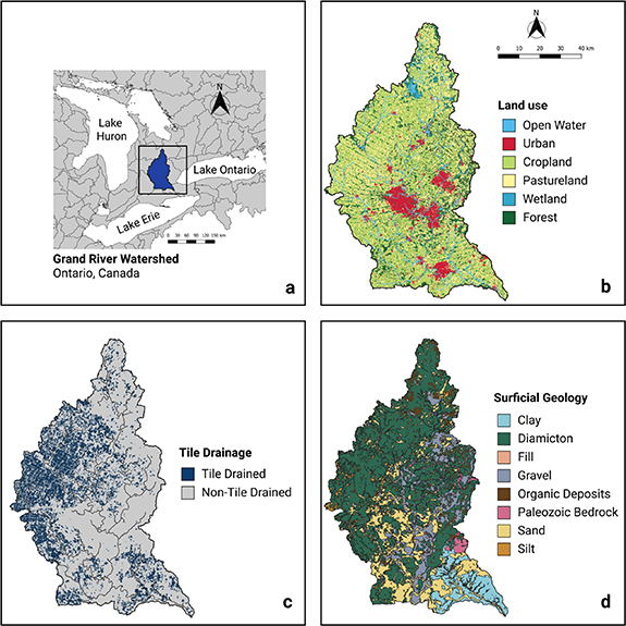
Figure 1. GRW (a) watershed location in the Lake Erie Basin; (b) land use map (AAFC 2016); (c) tile drainage map (Land Information Ontario 2018); (d) surficial geology (Ontario Geological Survey 2010).
Download figure:
Standard image High-resolution image3.2. Data sources
3.2.1. Watershed selection, streamflow and water quality data
Daily discharge data was obtained from the Canadian Hydrometric Database (Government of Canada 2021), while water quality data was obtained from the Provincial Water Quality Monitoring Network database (MOECC 2021). Water quality modelling stations were selected based on the following criteria: (a) availability of at least 20 years of data, and (b) proximity to a flow monitoring station. Flow and water quality stations were paired if there was a less than 10% difference in drainage areas. The 14 watersheds selected included six along the mainstem of the Grand and eight tributaries, and had 35–51 years of paired discharge and stream concentration data (figure 2). The basin characteristics for the 14 watersheds is presented in table S1. Daily nitrate concentrations (mg L−1) and loads (kg yr−1) were calculated from the continuous flow and sparse concentration data using the Weighted Regression on Time, Discharge and Season method (Hirsch et al 2010). The daily estimated nitrate concentration and discharge values were used to calculate annual dissolved N loads for each watershed.

Figure 2. The GRW stream network showing (a) mapped gauging station locations, where the colors of streams correspond to the colors of subbasin names in the flow chart, and (b) conceptual flow network.
Download figure:
Standard image High-resolution image3.2.2. N mass balance, land use and population data
Components of the N mass balance were calculated from 1700 to 2016 using county- and provincial-scale Canadian Agricultural Census data on fertilizer sales, livestock count and crop production, grid-scale N deposition data, and population data from the Canadian Census, following methodologies outlined in Byrnes et al (2020). Watershed land-use trajectories (1700–2016) were constructed using Annual Crop Inventory dataset (2011–2016) (AAFC 2016), supplemented by historical modeled cropland data from Ramankutty and Foley (1999) that provide gridded estimates of global cropland and pastureland area fractions for each year from 1700 to 2007 (SI text 1.1.1). Watershed N surplus trajectories were estimated as the sum of the N surplus on the different land use types (equations (3)–(5)) and domestic waste (supplemental section S1.2).
3.3. Sensitivity analyses, model calibration and uncertainty analyses
Global parameter sensitivity analysis was used to identify model parameters that have the most significant influence on SON content and stream N loading (Muleta and Nicklow 2005, Mishra 2009, Van Meter and Basu 2017) (SI text 2.1). The model was calibrated and validated based on (1) annual catchment N loads ( ) in equations (1) and (2) the watershed SON content. For annual catchment N loads, we used the Kling–Gupta Efficiency (KGE) (Gupta et al
2009) and percent bias (PBIAS) to test the goodness of fit of the data, while we used the PBIAS metric for SON. Higher KGE and lower PBIAS values indicate better model fit. The N loads were calibrated between 2000 and 2016, and validated between 1965 and 1999. Soil organic N was estimated from soil carbon data, assuming a C/N ratio of 14 (Cleveland and Liptzin 2007, AAFC, Soil Landscapes of Canada Working Group 2010).
) in equations (1) and (2) the watershed SON content. For annual catchment N loads, we used the Kling–Gupta Efficiency (KGE) (Gupta et al
2009) and percent bias (PBIAS) to test the goodness of fit of the data, while we used the PBIAS metric for SON. Higher KGE and lower PBIAS values indicate better model fit. The N loads were calibrated between 2000 and 2016, and validated between 1965 and 1999. Soil organic N was estimated from soil carbon data, assuming a C/N ratio of 14 (Cleveland and Liptzin 2007, AAFC, Soil Landscapes of Canada Working Group 2010).
Given the unique formulation of ELEMeNT, each of the 14 watersheds had to be modeled separately, and they were calibrated using the multi-objective optimization tool OSTRICH (Tolson and Shoemaker 2007, Asadzadeh and Tolson 2013, Matott 2017). We used a wider range of parameter values (table S2) for the headwater basins (figure 2), and a more constrained range for the downstream basins, such that a consistent relationship was retained among the parameters along the river network. We did 1000 OSTRICH runs for the upstream basins, and identified parameter sets with a KGE ⩾ 0.5 and a PBIAS ⩽ 10% for stream N loading, and a PBIAS ⩽ 25% for SON content. These ranges were used for the parameters for the downstream basins. The final parameter sets for all 14 watersheds were established by selecting the top-performing 4% of the parameter sets for KGE and 50% of the parameter sets for PBIAS—leading to 20–30 parameter sets for each basin. To address input uncertainty associated with the N surplus calculations, we performed Monte Carlo simulations for each of the 20–30 model parameter sets, and allowed the inputs to vary by assuming a normal probability distribution with a coefficient of variation of 0.3. Thus, we did 200–300 Monte Carlo runs for each of the 14 watersheds to quantify the effect of both parameter and input uncertainty.
Finally, while we used temporally constant parameter sets, it is possible that some of these parameters vary over time. This is especially true for the calibrated watershed mean travel time that can increase over time due to increasing tile drainage density over the last 60 years (Schilling et al 2012, Boland-Brien et al 2014, Van Meter and Basu 2017). Given that there is not much data available on tile drainage densities over time, we followed the work of Foufoula-Georgiou et al (2015), who found that extensive tile drain installation accompanied conversion of small grains to row crops in the Minnesota River Basin (Bajgain et al 2015). We identified land cover transition (LCT), as the point in time at which the area under row crops exceeds the land area planted in hay and small grains. To quantify the effect of tile density, we did a second calibration of the model prior to the LCT point, keeping all parameters constant and allowing only the mean travel time to be variable. This allowed us to compare the effect of changing tile density on calibrated travel times.
3.4. Future simulations
The ELEMeNT-N model was used to develop future scenarios of N reduction: (a) Business-As-Usual (Sc1); (b) a 50% reduction in the agricultural N surplus (Sc2): and (c) a 100% reduction in the agricultural N surplus (Sc3). The N surplus reduction was done uniformly over all cropland and pasture in each of the 14 watersheds. Future simulations were run assuming an intervention year of 2016.
4. Results and discussion
The objective of our study was to use a modeling framework, ELEMeNT-N, to quantify spatial patterns of legacy N accumulation, and to assess the impacts of these legacy sources on current and future water quality. We first synthesized land use, population and agricultural production data to create N surplus trajectories (section 4.1), which were then used to model N dynamics across the watershed (section 4.2). The model results were used to identify spatial patterns in the legacy N accumulation in soils and groundwater (section 4.3), and to quantify the effects of such accumulation on water quality trajectories (section 4.4).
4.1. Nitrogen surplus trajectories
The watershed-scale N surplus trajectories were found to be similar across the 14 subbasins of the GRW. Between 1900 and 1950, the N surplus in these watersheds remained relatively constant at less than 10 kg ha−1 yr−1; after 1950, however, surplus values began to increase, peaking in the late 1980s, and declining after that (figure 3(a)). The decrease in the N surplus is due primarily to increases in crop yield and decreases in atmospheric deposition rates across the basin (figure 3(b)). Notably, however, since the 2010s, the N surplus appears to be rising again, due to an increase in fertilizer application rates that has been observed across Canada (Dorff and Beaulieu 2014, Statistics Canada 2016). While N surplus trends are similar across the GRW, the actual N surplus magnitudes vary considerably (figure 3(a)), reaching as high as 69 kg ha−1 yr−1 in the agriculturally dominated Canagagigue Watershed (CA) to as low as 44 kg ha−1 yr−1 in the more wetland-dominated Marsville watershed (G1).
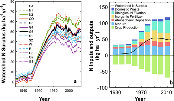
Figure 3. Watershed-scale N surplus trajectories: (a) watershed-scale N surplus trajectories for the GRW (Grand at York (G6), thick black line) and its 13 nested watersheds, (b) components of N inputs (fertilizer, biological N fixation, manure, atmospheric deposition, and domestic waste), and non-hydrologic outputs (crop N output) at the Grand at York. Bars are averages over 10 year time windows.
Download figure:
Standard image High-resolution imageBiological nitrogen fixation is currently the largest component of N inputs to the watershed, followed by manure, fertilizer, atmospheric deposition and human waste (figure 3(b)). The current importance of BNF stands in contrast to N inputs prior to 1950, when manure was the largest input, followed by BNF and fertilizer. This difference can be explained by the growing importance of soybean cultivation in the region (Bowley 2013). Indeed, area under soybean cultivation has increased by over 300% since the 1950s, while soybean yields have doubled, contributing to the observed increase in BNF over this timeframe. The domestic waste component of N inputs has also increased from previous decades due to rapid urbanization in the region, though the relative magnitude of N from human waste remains small at the watershed scale.
4.2. Model performance
The results of the sensitivity analysis indicate that our simulation of N loading at the catchment outlet ( ) in equation (1) is primarily controlled by denitrification rate constants in soil and groundwater (λs and γ), and the mean travel time (µ) through hydrologic pathways (table S3). In contrast, the median 1950–2016 SON levels are most sensitive to the pristine nitrogen content (Ms), the mineralization rate of active SON (ka), and the humification coefficient for cultivated land (hc). These findings are similar to those for the ELEMeNT-N models developed for the Mississippi and Susqehanna basins in the US (Van Meter et al
2017), highlighting that these controls are probably characteristic of these highly agricultural systems. Indeed, given the significantly large SON pool in the landscape, it is reasonable that N loads at the catchment outlet is less sensitive to the SON magnitude, and more sensitive to the travel time and the denitrification parameters that modulate the flux of mineral N during its transport from the root zone to the catchment outlet.
) in equation (1) is primarily controlled by denitrification rate constants in soil and groundwater (λs and γ), and the mean travel time (µ) through hydrologic pathways (table S3). In contrast, the median 1950–2016 SON levels are most sensitive to the pristine nitrogen content (Ms), the mineralization rate of active SON (ka), and the humification coefficient for cultivated land (hc). These findings are similar to those for the ELEMeNT-N models developed for the Mississippi and Susqehanna basins in the US (Van Meter et al
2017), highlighting that these controls are probably characteristic of these highly agricultural systems. Indeed, given the significantly large SON pool in the landscape, it is reasonable that N loads at the catchment outlet is less sensitive to the SON magnitude, and more sensitive to the travel time and the denitrification parameters that modulate the flux of mineral N during its transport from the root zone to the catchment outlet.
Model performance was evaluated based on simulations of annual catchment N loads (figure 4) as well as estimations of SON in the study watersheds. Median KGE values for the 14 study watersheds ranged between 0.65 and 0.95 during the calibration period, while the values were slightly lower during the validation periods (median range: 0.56–0.86) (table S4). It is likely that changing parameter values over time contributed to poorer metrics in the earlier time frame. We evaluated the effect of changing µ on improving PBIAS (section 3.3) in the validation period (1965–1999) in the eight watersheds with enough data in the pre-LCT years (table S5, figure 5(a)). The modification contributed to lower PBIAS values for all eight watersheds (table S4). The modeled results for SON content of the watersheds ranged from 6324 to 7532 kg ha−1, which were close to the measured values (table S4). The performance results are reasonable given the significant uncertainty in developing water quality models over decadal timescales.
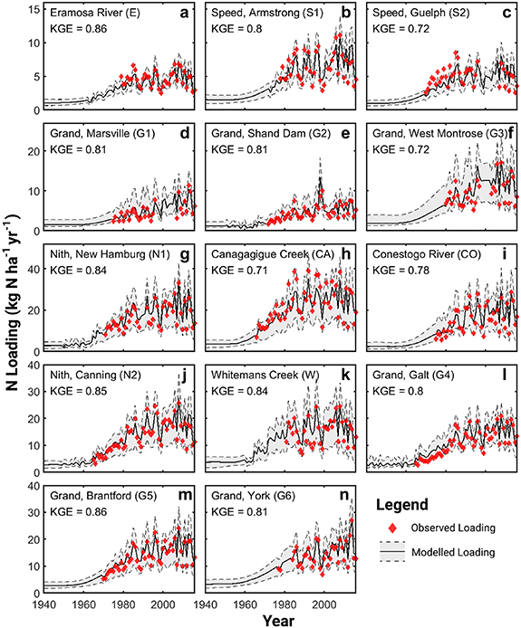
Figure 4. Catchment-scale dissolved N loading for the 14 study watersheds (1940–2010). Load values are normalized to the catchment area for the individual watersheds (kg ha−1 y−1). The black line represents the median of 200–300 Monte Carlo (MC) runs for each basin, considering both parameter and input uncertainty (see section 3.3), and the bounds of the grey areas indicate the upper and lower limits obtained from the MC runs. The red diamonds represent measured annual N loads.
Download figure:
Standard image High-resolution image
Figure 5. Effects of changing tile drainage density on the calibrated mean travel time µ: time trajectories of fraction of the watershed area under row crop and small grain to identify the LCT in (a) the Grand at Galt (G4); (b) Calibrated mean travel time before and after the LCT year in watersheds where a change point is identified; LCT year is in green.
Download figure:
Standard image High-resolution imageMean calibrated travel times ranged from 5 years for Canagagigue Creek to 34 years for the Speed River, soil denitrification rate constants ranged between 0.25 and 0.61 yr−1, while groundwater denitrification rate constants are lower and ranged between 0.07 and 0.1 yr−1 (table S6). For the five watersheds with positive PBIAS values, the calibrated µ values were 37%–67% greater before the LCT year (figure 5(b)), as would be expected for land with lower tile drainage densities (table S5, figure 5(b)). While it is well established that installation of tile drains decreases µ, and increases N loads (Blann et al 2009, Basu and Thompson 2011, Boland‐Brien et al 2014, Sloan et al 2016), our model's ability to capture this transition highlights the robustness of the long-term modelling approach. For the three watersheds with negative PBIAS values, the calibrated pre-LCT mu-values were actually lower. This result would suggest that travel times were actually faster during the period with less tile drainage, which does not make intuitive sense. In these watersheds, it is possible that temporal variability in other watershed drivers such as WWTP efficiency might be contributing to the observed results. There is not enough information, however, to more rigorously evaluate these other alternatives.
4.3. Nitrogen stores and fluxes along the river continuum
4.3.1. Nitrogen fluxes and stores in GRW subbasins
We next used the modeled results to estimate N stores and fluxes across the GRW. Over the last 86 years (1930–2016), the cumulative N surplus across the GRW has increased approximately linearly to 2952 kg ha−1 (figure 6(a)). This N surplus can have different fates. Across the GRW, we find that approximately 27% of the cumulative N surplus has been exported through the stream, while denitrification in soil and groundwater account for 35% of the surplus, and WWTP removal accounts for 10% of the N surplus. The remaining 30% of the N surplus, since 1940, is being stored within the landscape as legacy N (figure 6(a)). Of this, we estimate that 13% is stored in groundwater (106 kg ha−1), while the largest portion (87%) is stored in soil in the form of organic N (702 kg ha−1) (figure 6(a)). These magnitudes are significant, given current fertilizer application rates across the GRW of 36 kg ha−1 yr−1.

Figure 6. Cumulative N fluxes and stores in the GRW since 1930: (a) cumulative watershed-scale N surplus across the entire GRW from 1930 to present, and the component N stores (groundwater (GW) N accumulation and SON accumulation) and fluxes (stream N load, WWTP removal, landscape denitrification). (b) Proportion of the N stores and fluxes for various subbasins within the GRW Note landscape denitrification includes both soil and groundwater denitrification.
Download figure:
Standard image High-resolution imageThe proportions of these fluxes and stores vary in subbasins across the GRW as a function of variations in land use and land management. Specifically, the fraction of N being lost as riverine export ranges from 9% to 37%, while denitrification in the soil and groundwater accounts for 26%–53% of the N surplus, and WWTP removal accounts for 2%–12% of the surplus (figure 6(b)). Higher levels of stream export (25%–37%) are found in the heavily tile-drained, agricultural watersheds (e.g. Canagagigue Creek, the Conestogo River, Whitemans Creek), while watersheds with larger amounts of wetland coverage (Grand River at Marsville) have lower fractional export (14%). The findings of increased export with increasing tile drainage and decreasing wetland area is consistent with previous studies (Blann et al 2009, Hansen et al 2018). Less-developed subbasins like the Speed and Eramosa Rivers (tile drainage: 3%–8%) have relatively larger proportions N lost to landscape denitrification (45%–53%), with less riverine export (9%–13%). In these areas, lower tile-drainage densities possibly allow water to remain on the landscape longer, thus contributing to more denitrification (Boland‐Brien and Basu ). Legacy N stored in soil ranges between 21% and 47% of the N surplus, while 2% to 5% of the N surplus is stored in the groundwater (figure 6(b)).
4.3.2. Dominant controls on legacy N in soil and groundwater reservoirs and stream N load
The fraction of N surplus that accumulates in groundwater (fGW) was positively correlated with the calibrated mean travel time µ of the watershed (p = 0.06, R2 = 0.54), meaning that longer travel times correspond with greater accumulation magnitudes (table S7). This correlation highlights the importance of subsurface flow processes to the accumulation of groundwater legacy. No significant relationship was observed between fGW and any other model parameters. The fraction of the N surplus that accumulates as SON (fSON) correlated most strongly with µ (p = 0.02, R2 = 0.72; table S7), with a higher µ corresponding to areas with greater accumulation. Weaker, but still significant relationships were also observed between fSON and the mineralization rate constant (p = 0.06, R2 = 0.55, negative relationship), the soil denitrification rate constant (p = 0.08, R2 = 0.49, positive relationship), and the groundwater denitrification rate constant (p = 0.06, R2 = 0.54, positive relationship) (table S7). Note that, given significant uncertainty in modelled relationships, we use a more flexible criteria of p < 0.1 to assess the controls on legacy accumulation.
We next explored correlation relationships between watershed characteristics and the key model parameters (table S8). We found a significant relationship between µ, and both the soil type (% silt + clay) (R2 = 0.5, p = 0.07) and the tile-drainage density (R2 = 0.72, p = 0.02). We used the post-LCT µ in this analysis since the tile drainage density is only available for the current period. Notably, the relationship between the µ and the % silt + clay is a negative relationship, meaning that with a higher silt and clay content, the travel times are shorter. This finding is counter-intuitive, as soil physics suggest that travel times would be longer in less-permeable soils with a higher silt and clay content. However, this anomaly is easily explained by the strong positive relationship between µ, and the tile-drainage density. Tile drains short-circuit the slower subsurface flow pathways, and lead to shorter watershed travel times (Schilling et al 2012). Importantly, tile drains are also preferentially installed in soils with a high silt + clay content, as drainage in these soils is naturally poorer. The relationship here between soil type and µ is analogous to the empirical findings of Van Meter and Basu (2017), and it demonstrates the ability of the model to accurately capture processes associated with altered hydrological flow pathways across drained and undrained areas of the GRW.
Our modeling allowed us to capture important dynamics associated with human modification of the landscape, specifically the extensive installation of subsurface tile drainage to increase crop productivity (figure 7). First, increases in tile drainage lead to faster routing of subsurface N to the stream (Blann et al 2009, Basu and Thompson 2011, Foufoula-Georgiou et al 2015, Sloan et al 2017), and thus a decrease in the fraction of the surplus that accumulates in groundwater, as hydrologic legacy. Tile drainage also decreases the fraction of N surplus that accumulates as SON by changing the soil moisture conditions and the biogeochemical processes in the root zone of agricultural soils (Blann et al 2009). Specifically, an increase in tile-drained area can be associated with a lower water table which would increase mineralization rates and decrease denitrification rates due to more aerobic soils (Blann et al 2009), leading to a higher fraction of the N surplus being lost to riverine export (figure 7). Soil organic N accumulation rates could thus be lower in these drained aerobic soils, compared to more moist soils in areas that are non-tile drained. Thus, the fractional area in tile drains acts as the strongest control on fSON, with increase in tile drained area leading to a decrease in the SON accumulation. The dominant control of tile drainage on legacy accumulation has significant implications for watershed management. While it is well established that increasing tile density increases N loads, our results suggest that implementing watershed management in tiled areas would not only enable us to target hotspots in N pollution, but also lead to the fastest improvement in water quality as these regions are associated with lower legacy effects.

Figure 7. Drivers of legacy accumulation in soils and groundwater. Tile drainage decreases soil moisture, increases mineralization rates, decreases denitrification rates, increases N export and decreases legacy N accumulation.
Download figure:
Standard image High-resolution image4.3.3. Legacy stores along the river continuum
The correlation relationships developed in the previous section (table S7) are used along with the tile drainage maps to estimate watershed travel time maps across the GRW (figure 8(a)). The travel time maps are then used along with the cumulative N surplus maps (figure 8(b)), and the tile drainage maps to develop checkered landscapes that are characterized by heterogeneity in SON and groundwater nitrogen accumulation patterns across the GRW (figures 8(c) and (d)). High N surplus and shorter travel times in the southern part of the watershed contribute to greater legacy accumulation, while lower N surplus and longer travel times in the northern regions contribute to lower legacies.
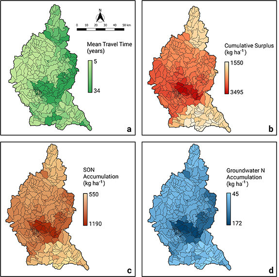
Figure 8. Spatial patterns of legacy accumulation along the GRW (1930–2016): (a) cumulative N surplus across the GRW, (b) mean travel time, (c) SON accumulation (d) groundwater N accumulation.
Download figure:
Standard image High-resolution image4.4. Future scenarios: nitrogen legacies and water quality trajectories
We first evaluated response at the outlet of the GRW, and found the Business-as-usual scenario (Sc1) to lead to a 4.8% decrease in N load from the 2008–2016 period mean load to the 2040 load (figure 9(a)). This decrease can be attributed to the decrease in N surplus magnitudes that has occurred since the 1980s. The 50% Agricultural Surplus Reduction (Sc2) and the 100% Agricultural Surplus Reduction scenarios (Sc3) led to somewhat proportional improvements in water quality with the decrease in N surplus (figure 9(a)). Such decreases in N surplus can be achieved through reductions in N fertilizer application, which would allow the crops to use the legacy reserves of SON in the soil. A targeted watershed management strategy that prioritizes sub basins with the largest N surpluses can be expected to yield the greatest water quality benefit.

Figure 9. Future simulation scenarios for the GRW and its subbasins. (a) Predicted N loads for the GRW under the future scenarios (Sc1: Business-as-usual, Sc2: 50% Agricultural Surplus Reduction; Sc3: 100% Agricultural Surplus Reduction). The grey region shows the uncertainty over the 20–30 accepted parameter sets (b) Percent N loading decrease in 2040 from the baseline (2008–2016) due to 50% N surplus reduction implemented in 2016, plotted as a function of legacy N accumulated in various sub basins within the GRW. Symbols without an outline are individual runs for the 20–30 parameter sets, while symbols with an outline represent the median response for that watershed. Higher mass of legacy N accumulation leads to a slower decrease in the N loading rate, and thus longer lag times (linear relationship; R2 = 0.06).
Download figure:
Standard image High-resolution image
Indeed, the responses were quite heterogeneous across the various subwatersheds of the GRW (figure 9(b)). What was really interesting was that the magnitude of reduction achieved was strongly controlled by the legacy accumulated. A higher legacy N in the watershed corresponded to a slower rate of loading decrease, ranging from 16% N loading decrease in 2040 in watersheds with 1150 kg ha−1 legacy N to 38% in watersheds with 670 kg ha−1 legacy N (figure 9(b)). A higher legacy N accumulation also corresponds to a longer lag time. For example, if the management goal is a 25% reduction in N load, then this will be achieved by 2040 (24 year lag time) in 10 of the 14 watersheds (according to their median run), while it would take longer in the other four watersheds. This analysis highlights the strong role legacy N plays in controlling both N load reduction, and the timescales of recovery following implementation of conservation measures.
5. Conclusion
Nitrogen legacies accumulate in the landscape over decades of agricultural intensification and lead to lag times in water quality improvement following implementation of BMPs. Design of appropriate watershed management strategies requires an understanding of the spatial patterns of legacy accumulation in heterogeneous landscapes, and quantification of the impacts of the legacy sources on water quality improvement trajectories. Here, we have demonstrated such an approach using a 6800 km2 agriculturally-dominated GRW in the Lake Erie Basin. We constructed 200 year N mass balance trajectories for 14 watersheds within the GRW, which were then used as inputs to the ELEMeNT-N model. The model was able to appropriately capture N loading trajectories across all 14 watersheds using only eight calibrated parameters. Model results were used to estimate legacy N accumulation that varied across the subbasins from 700 kg ha−1 in the Grand at Marsville to 1070 kg ha−1 in the Grand at Galt, and created a heterogeneous checkered landscape of N legacies. Spatially, magnitudes of legacy accumulation was strongly correlated with the presence of tile drainage, highlighting the strong anthropogenic control on nitrogen cycling.
SON accounted for the largest component of this legacy (82%–96%), and this form of legacy can potentially serve as a resource for crop growth, allowing us to achieve the same crop yields with lower fertilizer application rates (Venterea et al 2016, Banger et al 2020, Esmaeili et al 2020). Groundwater legacies are a smaller fraction (4%–18%), however, this legacy can only be addressed only by using downstream control measures such as wetlands and riparian buffers that intercepts the groundwater before it enters the river. Thus, though both soil and groundwater legacies can serve as a long-term source of N to surface waters; it is important to distinguish between the two, as management decisions may be different. Finally, we found that the timescales of water quality improvement were strongly correlated to the legacy accumulated, with higher legacy watersheds having longer lag times.
Our findings have significant implications with respect to watershed management to minimize lag times and reach water quality targets for N in agricultural watersheds. First, our results demonstrate that water quality improvement timescales, following implementation of conservation measures, are multidecadal and policy measures should take these timescales into account. Second, it demonstrates that management can be targeted to legacy hotspots, where the largest legacies have accumulated, to accelerate water quality improvement, instead of the current 'one-size-fits-all' approach. Having measurable success in management efforts can boost morale and encourage continued funding for long term water quality improvements. Such targeting strategies would theoretically result in the fastest and greatest response in stream N loading, and offer evidence for continuing long-term nutrient management plans needed for sustained water quality improvements.
Acknowledgement
We would like to acknowledge the anonymous reviewers for their help in improving this paper. This work was financed in part through the Natural Sciences and Engineering Research Council of Canada (NSERC) in the frame of the collaborative Water JPI international consortium pilot call under the project name 'Legacies of Agricultural Pollutants (LEAP): Integrated Assessment of Biophysical and Socioeconomic Controls on Water Quality Agroecosystems', and by Global Water Futures funds provided through the Canada First Research Excellence Fund.
Data availability statement
The data that support the findings of this study are available upon reasonable request from the authors.
Datasets for this research are available in these in-text data citation references: Ramankutty and Foley (1999); AAFC (2015, 2016); Land Information Ontario (2018); Ontario Geological Survey (2010); Statistics Canada (2016a, 2016b, 2017a, 2017b), Hember (2018).