


1. Introduction
Electrophoresis is characterized as the motion of charged particles under the action of externally imposed electric fields in a liquid medium (Levich Reference Levich1962; Saville Reference Saville1977; Anderson Reference Anderson1985; Ohshima Reference Ohshima1996; Yariv & Brenner Reference Yariv and Brenner2003; Ohshima Reference Ohshima2006; Khair & Squires Reference Khair and Squires2009; Schnitzer et al. Reference Schnitzer, Zeyde, Yavneh and Yariv2013; Schnitzer & Yariv Reference Schnitzer and Yariv2014; Goswami et al. Reference Goswami, Dhar, Ghosh and Chakraborty2017), which may or may not contain ions in the form of electrolytes (Saville Reference Saville1977; Ohshima Reference Ohshima2006). This phenomenon has been a prominent area of research over decades owing to its wide gamut of applications such as colloid science (Ohshima Reference Ohshima2006; Khair, Posluszny & Walker Reference Khair, Posluszny and Walker2012) and separation of particles (Ghosal Reference Ghosal2006), DNA analysis (Khair & Squires Reference Khair and Squires2009), gel electrophoresis (Babnigg & Giometti Reference Babnigg and Giometti2004), particle deposition (Besra & Liu Reference Besra and Liu2007) among many others. In many instances, electrophoretic motion occurs in complex media (Ramautar, Demirci & de Jong Reference Ramautar, Demirci and de Jong2006), such as bio-fluids (Babnigg & Giometti Reference Babnigg and Giometti2004; Kremser, Blaas & Kenndler Reference Kremser, Blaas and Kenndler2004), polymeric solutions (Li & Koch Reference Li and Koch2020; Barron, Sunada & Blanch Reference Barron, Sunada and Blanch1995) etc., whose constitutive behaviours show strong deviations from the Newtonian paradigm. These facets have been progressively becoming important in recent times (Berli Reference Berli2010; Bandopadhyay & Chakraborty Reference Bandopadhyay and Chakraborty2012b; Bandopadhyay, Ghosh & Chakraborty Reference Bandopadhyay, Ghosh and Chakraborty2013; Zhao & Yang Reference Zhao and Yang2013; Ghosh & Chakraborty Reference Ghosh and Chakraborty2015; Ghosh, Chaudhury & Chakraborty Reference Ghosh, Chaudhury and Chakraborty2016), because of their key roles in medical diagnostics (Madou et al. Reference Madou, Lee, Daunert, Lai and Shih2001; Groisman, Enzelberger & Quake Reference Groisman, Enzelberger and Quake2003), particle focusing (Lu et al. Reference Lu, DuBose, Joo, Qian and Xuan2015), efficient micromixing (Lam et al. Reference Lam, Gan, Nguyen and Lie2009) to name a few. Some such specific applications include: gel electrophoresis for proteome sequencing (Babnigg & Giometti Reference Babnigg and Giometti2004), capillary electrophoresis for separation and purification of biological substances (Karger, Cohen & Guttman Reference Karger, Cohen and Guttman1989; Kremser et al. Reference Kremser, Blaas and Kenndler2004; Ramautar et al. Reference Ramautar, Demirci and de Jong2006), measurements of large aggregates of viruses, bacteria and eukaryotic cells (Kremser et al. Reference Kremser, Blaas and Kenndler2004) among others.
It is well established that fluid media of emerging interest in electrically mediated transport of biological entities commonly exhibit viscoelastic behaviour (Skalak, Ozkaya & Skalak Reference Skalak, Ozkaya and Skalak1989; Brust et al. Reference Brust, Schaefer, Doerr, Pan, Garcia, Arratia and Wagner2013). However, a majority of studies on electrophoresis (Saville Reference Saville1977; Baygents & Saville Reference Baygents and Saville1991; Ohshima Reference Ohshima2006; Khair & Squires Reference Khair and Squires2009) tend to focus on particle motion in Newtonian fluids, while only a handful of investigations (Hsu, Yeh & Ku Reference Hsu, Yeh and Ku2006; Hsu & Yeh Reference Hsu and Yeh2007; Khair et al. Reference Khair, Posluszny and Walker2012; Posluszny Reference Posluszny2014; Li & Koch Reference Li and Koch2020) have addressed the phenomenon in a non-Newtonian medium. Among those, many of the investigations concern Carreau-type constitutive models (Bird, Armstrong & Hassager Reference Bird, Armstrong and Hassager1987; Khair et al. Reference Khair, Posluszny and Walker2012), which are designed to capture the shear dependent viscosity exhibited by many polymeric liquids, but are unable to describe many other important characteristics (such as the ‘normal stress effects’) exhibited by such liquids (Bird et al. Reference Bird, Armstrong and Hassager1987; Ghosh et al. Reference Ghosh, Chaudhury and Chakraborty2016). On the other hand, viscoelastic constitutive models, such as the retarded motion relations (Chan & Leal Reference Chan and Leal1979) as well as the differential constitutive relations (Bird et al. Reference Bird, Armstrong and Hassager1987; Mukherjee & Sarkar Reference Mukherjee and Sarkar2010; Ghosh & Chakraborty Reference Ghosh and Chakraborty2015), hold certain favourable characteristics in capturing many of the essential rheological features of various polymeric (Bird et al. Reference Bird, Armstrong and Hassager1987; Barron et al. Reference Barron, Sunada and Blanch1995; Li & Koch Reference Li and Koch2020) as well as biological fluids (Yeleswarapu et al. Reference Yeleswarapu, Kameneva, Rajagopal and Antaki1998; Brust et al. Reference Brust, Schaefer, Doerr, Pan, Garcia, Arratia and Wagner2013). As a result, numerous types of viscoelastic flows have been widely studied (for instance, Vamerzani, Norouzi & Firoozabadi Reference Vamerzani, Norouzi and Firoozabadi2014; Turkoz et al. Reference Turkoz, Lopez-Herrera, Eggers, Arnold and Deike2018) over the years, although rigorous studies on electrophoretic motion through viscoelastic medium are extremely scarce. Lu et al. (Reference Lu, Patel, Zhang, Woo Joo, Qian, Ogale and Xuan2014, Reference Lu, DuBose, Joo, Qian and Xuan2015) have carried out experiments on capillary electrophoresis in viscoelastic fluids, wherein intriguing streamwise particle oscillations were reported that are otherwise not witnessed in Newtonian media. Very recently, Li & Koch (Reference Li and Koch2020) have theoretically investigated electrophoresis in dilute polymer solutions for a uniformly charged particle and predicted a reduction in the electrophoretic mobility because of the polymeric stresses inside the electrical double layer (EDL).
Another important feature of most of the reported theoretical studies on electrophoresis is that they mainly focus on spherical particles with uniform surface charge density (Saville Reference Saville1977; Ohshima Reference Ohshima2006; Khair & Squires Reference Khair and Squires2009; Li & Koch Reference Li and Koch2020). However, in many cases, the moving particles might have non-uniformly distributed charges on their surfaces, either naturally induced or externally imposed. As Anderson (Reference Anderson1985) points out, phenomena like heterocoagulation and crystallinity may lead to non-uniform charge density on a particle's surface. In addition, particles like bacterial cells and DNA (Amro et al. Reference Amro, Kotra, Wadu-Mesthrige, Bulychev, Mobashery and Liu2000; Velegol Reference Velegol2002), various inorganic particles (Van Riemsdijk et al. Reference Van Riemsdijk, Bolt, Koopal and Blaakmeer1986; Velegol Reference Velegol2002) and particles with adsorbed surfactants (Fleming, Wanless & Biggs Reference Fleming, Wanless and Biggs1999) might naturally exhibit non-uniform surface charge density. At the same time, ‘Janus particles’ (Molotilin, Lobaskin & Vinogradova Reference Molotilin, Lobaskin and Vinogradova2016) might be artificially engineered to have varying surface properties, which may lead to non-uniform surface charges among other features. In view of such prevalence of non-uniformly charged particles, several studies (Anderson Reference Anderson1985; Yoon Reference Yoon1991; Velegol Reference Velegol2002) have been carried out to derive expressions for their electrophoretic mobility, albeit exclusively in Newtonian fluids. Several researchers have also probed the mobility of non-spherical particles (Fair & Anderson Reference Fair and Anderson1989; Solomentsev & Anderson Reference Solomentsev and Anderson1994; Yariv Reference Yariv2005). While these studies clearly predict that the non-uniformity in the surface charge alters the electrophoretic mobility, the underlying implications in non-Newtonian fluid medium have not yet been probed.
The interactions between the viscoelastic polymeric stresses and the Maxwell stresses within the EDL would fundamentally alter the flow dynamics within the same, and hence hold the potential of resulting in substantial alterations in fluid motion around the particle. Considering that perspective and realizing an effective compromise between rheological complexity and analytical tractability, here, we analyse electrokinetics around a non-uniformly charged spherical particle in a viscoelastic medium, whose constitutive behaviour is given by the Oldroyd-B model. This constitutive relation is chosen over the ordered-fluid models, because of its applicability to flows with comparatively higher strain rates (Bird et al. Reference Bird, Armstrong and Hassager1987).
We confine our attention to the thin EDL limit (thin EDL) (Ajdari Reference Ajdari1995; Mandal et al. Reference Mandal, Ghosh, Bandopadhyay and Chakraborty2015) and first formulate a generalized framework to evaluate the modified Smoluchowski slip velocity around the particle with arbitrary non-uniform surface charge. In order to work with a closed-formed theoretical framework, we assume the particle to be weakly charged; however, the surface charge is otherwise arbitrary and non-uniform. We illustrate that, for weak surface charge, the viscoelastic effects become subdominant in the leading-order asymptotes, which essentially results in a small effective Deborah number ( $De_{eff}$, defined later).
As simple applications of the modified Smoluchowski slip thus derived, we consider two specific case studies. First, we explore the electrophoretic translation of a non-uniformly but axisymmetrically charged particle. Second, we probe the pure electrophoretic rotation of a non-uniformly and non-axisymmetrically charged particle in a viscoelastic medium. The analysis is carried out by using a combination of singular and regular asymptotic expansions. Noting that the applicability of Oldroyd-B model becomes questionable at relatively moderate to large dimensionless relaxation times, as expressed in terms of Deborah numbers (defined later), we further report numerical solutions of the physical problem by employing an illustrative nonlinear viscoelastic model, namely, the finitely extensible nonlinear elastic (FENE-P) model, in appropriate limiting scenarios. Subsequent comparisons reveal that the predictions using the Oldroyd-B model agree reasonably well with the FENE-P model as long as the surface charge is weak and the maximum allowed polymer lengths are large. One of the main goals of the case studies stated above is to bring out the unique effects of non-uniform charge density on the particle's mobility in a viscoelastic fluid. To this end, it is demonstrated that the electrophoretic mobility (both translational and angular velocities) of the particle strongly depends on the non-uniformity of the surface charge, the relaxation and retardation times scales as well as the particle's curvature and may lead to breaking of fore–aft symmetry even for viscous flows in the low surface charge limits, which is in stark contrast to what is witnessed in Newtonian fluids. We successfully demonstrate that, under appropriate limiting conditions, previously reported results for Newtonian as well as viscoelastic fluids can be recovered as special cases of our theoretical framework.
The rest of the paper is organized as follows. In § 2, we provide a basic outline of the problem statement, the fundamental governing equations and the essential force and torque balance around the particle. In § 3, the modified Smoluchowski slip velocity is computed in the thin EDL limit for effectively weak viscoelastic flows. A more complete theoretical foundation, which includes the effects of rotation at higher orders of expansion, is presented in the supplementary material available at https://doi.org/10.1017/jfm.2021.643. In § 4, a model example of a non-uniformly charged particle is considered and its electrophoretic mobility is obtained based on the developed theory. Further, subsequent comparisons with reported results are carried out, to benchmark the theoretical framework as well as to bring out some of the novel insights specific to our study. In § 5, we explore how viscoelasticity changes the particle's angular velocity at a given instant, wherein the particle carries a non-axisymmetric surface charge. In § 6, we shed light on a potential experimental set-up, which may be used to validate some of the key predictions of our analysis. Finally, in § 7, concluding remarks are presented.
2. The physical paradigm and the governing equations
2.1. Description of the system
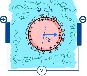
The prototypical system, as shown schematically in figure 1, consists of a spherical particle of radius  $a$, carrying an arbitrary non-uniform surface charge of density
  $\sigma '(\theta ,\varphi )$, suspended in a viscoelastic medium of viscosity
  $\eta$, permittivity
  $\varepsilon$, relaxation time (Bird et al. Reference Bird, Armstrong and Hassager1987)
  $\lambda '_1$ and a retardation time
  $\lambda '_2$. The fluid also contains dissolved electrolytes, which dissociate into ions and form an EDL around the particle surface (Ohshima Reference Ohshima2006; Poddar et al. Reference Poddar, Maity, Bandopadhyay and Chakraborty2016), as shown in the schematic. The electrolyte concentration away from the particle is
  $c'_0$. The fluid is assumed to obey the Oldroyd-B constitutive relation. A uniform electric field (i.e. uniform only far away from the particle) of magnitude
  $E_0$ is applied to actuate motion. Without loss of generality, we may choose the direction of the applied field to be the
  $z$-axis. The variables around the particle are expressed using a spherical polar coordinate (
 $r',\theta ,\varphi$), with the origin fixed at the particle's centre, translating but not rotating with it.

Figure 1. Schematic of a spherical particle of radius  $a$, carrying an arbitrary surface charge density
  $\sigma '(\theta ,\varphi )$. The particle is translating with velocity
  $\mathcal {U'}{\hat {\boldsymbol {e}}}_u$ in a viscoelastic medium, subject to an externally applied electric field (magnitude far from the particle
  $E_0$) along the
  $z$ direction. The fluid has viscosity
  $\eta$, relaxation time
  $\lambda '_1$, retardation time
  $\lambda '_2$ and permittivity
  $\varepsilon$.
As a result of the electrical forces acting on the particle, it will move with a velocity  $\mathcal {U}'{\hat {\boldsymbol {e}}}_u$, where
  ${\hat {\boldsymbol {e}}}_u$ is the unit vector pointing towards the direction of the particle's motion. In general,
  ${\hat {\boldsymbol {e}}}_u$ is not constrained to be oriented along the
  $z$-axis (Anderson Reference Anderson1985). In addition, because of non-uniform surface charge, the particle may also undergo rotational motion (Anderson Reference Anderson1985; Yoon Reference Yoon1991; Solomentsev & Anderson Reference Solomentsev and Anderson1994) with angular velocity
  $\boldsymbol {\varOmega }'$, much like other anisotropic particles.
Noting that analysis of electrophoretic motion is quite a formidable problem (Saville Reference Saville1977), several physically realistic assumptions may be made (Ohshima Reference Ohshima1996, Reference Ohshima2015; Schnitzer et al. Reference Schnitzer, Zeyde, Yavneh and Yariv2013), which can simplify the underlying governing equations significantly, improving analytical tractability in the process. In the same spirit, we also apply a few simplifying assumptions, keeping in mind that our main goal here is to assess the role of viscoelasticity in the presence of non-uniform surface charge.
First, we shall assume the surface charge density to be weak for analytical tractability without sacrificing the essential physics of interest –we quantify the specific regime qualifying this ‘weak’ surface charge limit later. Second, we assume the characteristic EDL thickness ( $\lambda _D$) to be much smaller than the particle's radius (
 $a$), which is a reasonably valid assumption for most practical considerations, since the EDL thickness typically lies in the tune of
  ${\sim }1 - 100\ \textrm {nm}$ (Ajdari Reference Ajdari1995; Bandopadhyay & Chakraborty Reference Bandopadhyay and Chakraborty2012a). Third, we assume that the ionic Péclet number (denoted by
  $Pe = u_c a/D'$;
  $u_c$ being the characteristic velocity, as defined later,
  $D'$ being the ionic diffusivity), as well as the dimensionless applied external field (as defined later), to be of the order of unity or less. This is in line with the consideration that for most particles,
  $Pe\sim O(1)$ (Saville Reference Saville1977). Fourth, the dimensionless relaxation time of the fluid medium as expressed in terms of the nominal Deborah number (
 $De$, see § 2.2 for definition) remains
  $O(1)$ or less. Despite invoking this consideration, later in § 3.4 we establish that, because of the weak surface charge limit (see the first assumption), the dimensionless velocity scale itself is less than
  $O(1)$, and hence the effective Deborah number (denoted as
  $De_{eff}$ later) is rendered much smaller than unity. As a consequence, the overall flow is only weakly viscoelastic, i.e. linear contributions dominate the leading-order flow stresses. Hence, the mathematical analysis carried out herein is very similar to an ordered-fluid expansion around the Newtonian limit (Chan & Leal Reference Chan and Leal1979). However, the Oldroyd-B constitutive relation is used because of its larger range of applicability as compared with an ordered fluid, which remains valid only for low strain rates (Bird et al. Reference Bird, Armstrong and Hassager1987). Fifth, we shall disregard the presence of a depletion layer (Pranay, Henríquez-Rivera & Graham Reference Pranay, Henríquez-Rivera and Graham2012; Mukherjee et al. Reference Mukherjee, Das, Dhar, Chakraborty and DasGupta2017) and assume the entire medium to exhibit viscoelastic characteristics. This requires that the characteristic EDL thickness be much larger than the polymer characteristic dimensions so that the continuum approximation remains valid inside the EDL. Towards assessing the validity of this assumption, one may refer to the radius of gyration (
 $R_g$) of the polymer as its representative length scale, which is a measure of the length scale of its random coil shapes (Israelachvili Reference Israelachvili2011). To compare physically realistic values of
  $R_g$ with those of
  $\lambda _D$ (the characteristic EDL thickness), we consider the example of poly-ethylene glycol in water (Cruje & Chithrani Reference Cruje and Chithrani2014). With a monomer length of
  ${\approx }0.35\ \textrm {nm}$ for
  $n = 100$ segments, one arrives at
  $R_g \approx 1.43\ \textrm {nm}$; for
  $n = 1000$ segments,
  $R_g \approx 4.5\ \textrm {nm}$. Therefore, for
  $\lambda _D \sim O(10\ \text {nm})$, the EDL thickness is an order of magnitude larger than the radius of gyration, which should safely allow us to assume a continuum distribution of polymers inside the Debye layer, as has been considered in a number of previous studies (Afonso, Alves & Pinho Reference Afonso, Alves and Pinho2009; Li & Koch Reference Li and Koch2020). Further, in practice, the polymer molecule includes only a tiny fraction of the random coil structure, which further justifies this continuum approximation. Finally, for a rotating particle (i.e.
  $\boldsymbol {\varOmega } \neq 0$), its surface charge distribution may be time variant. Although in § 5 we shall consider rotating particles, we will neglect such a dynamically evolving surface charge for the theoretical derivations. Nevertheless, an outline of time variation of the surface charge due to rotation has been provided in § S1 of the supplementary material accompanying this manuscript.
2.2. The characteristic scales
Electrophoretic motion entails several important characteristic scales for a number of different variables, dictating the flow dynamics. For any variable  $\xi '$, we denote it's characteristic scale by
  $\xi _c$. As such, the following characteristic scales are chosen: the characteristic potential:
  $\psi _c = kT/e$ (where k is the Boltzmann constant, T is the absolute temperature and e the protonic charge) – this is the thermal potential; the characteristic length:
  $r_c = a$; the characteristic velocity: (Saville Reference Saville1977),
  $u_c = {\varepsilon k^{2} T^{2}}/{e^{2}\eta a}$; the characteristic concentration:
  $c_c = c'_0$. Based on these choices, the characteristic stress reads:
  $\tau _c = \eta u_c/a$, whereas the characteristic surface charge is
  $\sigma _c$. Finally, the characteristic relaxation time may be equated to
  $\lambda _0 =\max (\lambda '_1,\lambda '_2)$.
A number of important non-dimensional numbers emerge from the above characteristic scales, which strongly influence the flow around the particle. These include: (i) the characteristic EDL thickness,  $\lambda _D = \sqrt {{\varepsilon k T}/{2c'_0 e^{2}}}$, with
  $\delta = \lambda _D/a$ – as the non-dimensional EDL thickness; (ii) the characteristic surface potential of the particle (Ajdari Reference Ajdari1995),
  $\zeta _c = \sigma _c \lambda _D/\varepsilon$, with
  $\bar {\zeta }_0 = e\zeta _c/kT$ as the characteristic potential relative to the thermal potential; (iii) the relative strength of the external field may be expressed through (Saville Reference Saville1977)
  $\beta = e E_0 a/kT$; (iv) the ionic Péclet number may be defined as (Saville Reference Saville1977)
  $Pe = u_c a/D$; (v) the nominal Deborah number, which indicates the extent of departure from Newtonian behaviour, may be defined as
  $De = u_c \lambda _0/a$. While various alternative approaches to quantify the extent of viscoelasticity have been reported (Li & Koch Reference Li and Koch2020); also see § 4.3 for further discussion, the advantage of defining
  $De$ using
  $u_c$ mentioned as above lies in the fact that various important asymptotic limits (such as weak surface charge, weak field limit, thin EDL limit etc.) may be independently explored without necessitating alteration to the magnitude of the Deborah number under consideration. In other words, the effect of electrokinetics may be elegantly isolated without requiring us to alter the quantitative representation of the fluid constitution.
Various assumptions stated in § 2.1 are now quantified in terms of the relevant non-dimensional numbers. ‘Weak surface charge’ indicates,  $\bar {\zeta }_0 \ll 1$; ‘thin EDL’ implicates
  $\delta \ll 1$; the strengths of advection and applied field are constrained by:
  $\beta \sim O(1)$ and
  $Pe\sim O(1)$. It needs to be clarified here that, despite
  $De \sim O(1)$, the limit of weak surface charge (
 $\bar {\zeta }_0\ll 1$) implies that the dimensionless electrokinetic velocity would scale as
  $O(\bar {\zeta }_0)$. Therefore, the confluence of electromechanics and hydrodynamics would lead to an effective Deborah number given by
  $De_{eff}\sim O(\bar {\zeta }_0 De) \ll 1$ – see §§ 3.4 and 3.5. Accordingly, the effect of viscoelasticity remains subdominant in the theoretical derivations of the flow field under weak surface charge limits, despite the nominal
  $De$ being
  ${\sim }O(1)$. As a consequence, it is not necessary to further assume low polymer concentration (Li & Koch Reference Li and Koch2020), which would require
  $\lambda '_1/\lambda '_2-1\ll 1$ – see § 3.5 for further discussion of this.
2.3. The governing equations
The transport processes are governed by the Poisson–Nernst–Planck–Cauchy momentum equations (Saville Reference Saville1977; Ghosh et al. Reference Ghosh, Chaudhury and Chakraborty2016), along with the continuity equation for conservation of mass and the Oldroyd-B constitutive equations. Since these equations are well established, we directly start with their dimensionless forms, wherein the non-dimensional version of the any variable  $\xi '$ is expressed as
  $\xi = \xi '/\xi _c$. The Nernst–Planck equations are reformulated in terms of the net charge density and concentration, defined as (Schnitzer & Yariv Reference Schnitzer and Yariv2014)
  $c = c_{+}+c_{-}$ and
  $\rho = c_{+}-c_{-}$ respectively, where
  $c_{+(-)}$ is the concentration of the positive (negative) ions. In view of the characteristic scales outlined in § 2.2, the governing equations are written as (Saville Reference Saville1977; Bird et al. Reference Bird, Armstrong and Hassager1987)
 \begin{gather} Pe({\boldsymbol{v}}\boldsymbol{\cdot}\boldsymbol{\nabla} c) = \nabla^{2} c+\boldsymbol{\nabla} \boldsymbol{\cdot}\left\{\rho\boldsymbol{\nabla}\psi\right\}, \end{gather}
 \begin{gather}Pe({\boldsymbol{v}}\boldsymbol{\cdot}\boldsymbol{\nabla} \rho) = \nabla^{2} \rho+\boldsymbol{\nabla} \boldsymbol{\cdot}\left\{c\boldsymbol{\nabla}\psi\right\} , \end{gather}
 \begin{gather}\delta^{2}\nabla^{2}\psi ={-}\tfrac{1}{2}\rho, \end{gather}
 \begin{gather}-\boldsymbol{\nabla} p + \boldsymbol{\nabla}\boldsymbol{\cdot}\boldsymbol{\tau} +\nabla^{2}\psi\boldsymbol{\nabla} \psi = 0 \quad \text{and} \quad \boldsymbol{\nabla}\boldsymbol{\cdot}{\boldsymbol{v}} = 0, \end{gather}
 \begin{gather}\boldsymbol{\tau} + De\lambda_1 \overset{\nabla}{\boldsymbol{\tau}} = 2{\boldsymbol{D}} + 2\lambda_2 De \overset{\nabla}{{\boldsymbol{D}}} . \end{gather}
In the above equations,  $\boldsymbol {\tau }$ is the stress field,
  $p$ is the pressure,
  $\psi$ is the electrical potential,
  ${\boldsymbol {D}}$ is the rate of strain tensor (
 ${=}\frac {1}{2}[\boldsymbol {\nabla }{\boldsymbol {v}} + (\boldsymbol {\nabla }{\boldsymbol {v}})^\textrm {T}]$) and
  ${\boldsymbol {v}}$ is the velocity field. Further,
  $\overset {\nabla }{\boldsymbol {\tau }}$ and
  $\overset {\nabla }{{\boldsymbol {D}}}$ indicate the first convected derivatives of the stress and strain rate. For any second-rank tensor
  ${\boldsymbol {A}}$, it's convected derivative
  $\overset {\nabla }{{\boldsymbol {A}}}$ is expressed as (Bird et al. Reference Bird, Armstrong and Hassager1987)
  $\overset {\nabla }{{\boldsymbol {A}}} = {\textrm {D}{\boldsymbol {A}}}/{\textrm {D}t}-(\boldsymbol {\nabla }{\boldsymbol {v}})^\textrm {T}\boldsymbol {\cdot }{\boldsymbol {A}}-{\boldsymbol {A}}\boldsymbol {\cdot }\boldsymbol {\nabla }{\boldsymbol {v}}$. The above equations are subject to the following boundary conditions:
 \begin{gather} {\hat{\boldsymbol{e}}}_r\boldsymbol{\cdot}\left[Pe{\boldsymbol{v}} c - \boldsymbol{\nabla} c -\rho\boldsymbol{\nabla}\psi\right]_{r=1} = {\hat{\boldsymbol{e}}}_r\boldsymbol{\cdot}\left[Pe{\boldsymbol{v}} \rho - \boldsymbol{\nabla} \rho -c\boldsymbol{\nabla}\psi\right]_{r=1} = 0 \end{gather}
 \begin{gather}{\hat{\boldsymbol{e}}}_r\boldsymbol{\cdot}[\boldsymbol{\nabla}\psi]_{r=1} ={-}\frac{\zeta(\theta,\varphi)}{\delta};\quad \zeta = \frac{\sigma'\lambda_D e}{\varepsilon kT}\quad \text{and}\quad [\boldsymbol{\nabla}\psi]_{r\rightarrow\infty} ={-}\beta{\hat{\boldsymbol{e}}}_z \end{gather}
 \begin{gather}{\boldsymbol{v}}(r=1,\theta,\varphi) = \boldsymbol{\varOmega}\times {\hat{\boldsymbol{e}}}_r\quad \text{and}\quad {\boldsymbol{v}}(r\rightarrow\infty,\theta,\varphi) ={-}\mathcal{U}{\hat{\boldsymbol{e}}}_u \end{gather}
 \begin{gather}\text{at}\ r\rightarrow \infty, \ c = 2 \quad \text{and}\quad \rho = 0. \end{gather}
Note that, in (2.2c), the boundary condition for velocity at the particle surface accounts for its rotation. In (2.2b),  $\zeta (\theta ,\varphi )$ is analogous to the surface potential and
  $\zeta \sim O(\bar {\zeta }_0)$ is it's characteristic magnitude. For convenience, we define,
  $\zeta (\theta ,\varphi ) = \bar {\zeta }_0\bar {\zeta }(\theta ,\varphi )$, such that
  $\bar {\zeta } \sim O(1)$. For electrophoretic motion,
  $\mathcal {U}{\hat {\boldsymbol {e}}}_u$ and
  $\boldsymbol {\varOmega }$, i.e. the migration velocity of the particle and it's angular velocity are the primary unknowns. To compute them, we simply need to balance the force and the moment around the origin, acting on the particle at steady state. The resulting balances are as follows (Anderson Reference Anderson1985; Ohshima Reference Ohshima2006; Goswami et al. Reference Goswami, Dhar, Ghosh and Chakraborty2017):
 \begin{gather} -\frac{\bar{\zeta}_0}{\delta}\int_{S_p} \bar{\zeta}\boldsymbol{\nabla}\psi \,\textrm{d}S + \int_{S_p} \boldsymbol{\tau}\boldsymbol{\cdot}{\hat{\boldsymbol{e}}}_r \,\textrm{d}S = 0, \end{gather}
 \begin{gather}-\frac{\bar{\zeta}_0}{\delta}\int_{S_p} \bar{\zeta}({\hat{\boldsymbol{e}}}_r\times\boldsymbol{\nabla}\psi) \,\textrm{d}S + \int_{S_p} {\hat{\boldsymbol{e}}}_r\times\left(\boldsymbol{\tau}\boldsymbol{\cdot}{\hat{\boldsymbol{e}}}_r\right) \textrm{d}S = 0 . \end{gather}
It is important to note here that the above ‘force-free’ conditions only remain valid in an unbounded medium, as previously noted by Yariv (Reference Yariv2006). Presence of a wall sufficiently close to the particle may change the force balance on the same.
The first terms in the above equations represent the force and the moment, respectively, due to the electric field. The second terms are essentially contributed by the stresses in the fluid. The integration is carried out over the particle surface  $S_p$. In the limit of a thin EDL, i.e. for
  $\delta \rightarrow 0$, the EDL may also be included within
  $S_p$ so that the integration is carried out on a surface just outside the EDL (as
  $\delta \rightarrow 0$, the EDL effectively has zero thickness). Since the net charge in the EDL and on the particle surface are opposite and equal, the net charge on an imaginary surface just outside of the EDL would be zero. Therefore, the first terms in both (2.3a) and (2.3b) vanish (Ye et al. Reference Ye, Sinton, Erickson and Li2002; Chen & Keh Reference Chen and Keh2014) and, as a result, the net force and moment caused by the stresses in the fluid on the imaginary sphere lying just outside the EDL (i.e. on the object
  $\textrm {particle}+\textrm {the}$ EDL) becomes zero (Ye et al. Reference Ye, Sinton, Erickson and Li2002; Chen & Keh Reference Chen and Keh2014). Equations (2.3a) and (2.3b) may then be re-written as
 \begin{equation} \int_{S_p} \boldsymbol{\tau}\boldsymbol{\cdot}{\hat{\boldsymbol{e}}}_r \,\textrm{d}S = 0\quad \text{and}\quad \int_{S_p} {\hat{\boldsymbol{e}}}_r\times (\boldsymbol{\tau}\boldsymbol{\cdot}{\hat{\boldsymbol{e}}}_r) \,\textrm{d}S = 0. \end{equation}
Notice that the integration is to be performed over the surface  $S_p$, which has a radius
  $r \sim 1+\delta$ and includes the EDL as well.
Finally, we note that the potential may be conveniently split into two parts as follows (Bahga, Vinogradova & Bazant Reference Bahga, Vinogradova and Bazant2010; Ghosh, Mandal & Chakraborty Reference Ghosh, Mandal and Chakraborty2017):  $\psi = \phi + \phi _{ext}$, where
  $\phi _{ext}$ is the contribution from only the externally imposed electric field and
  $\phi$ is the contribution of the particle's surface charge to the total electrostatic potential. It may then be deduced that
  $\phi _{ext}$ satisfies the equation (Ghosh et al. Reference Ghosh, Mandal and Chakraborty2017)
  $\nabla ^{2}\phi _{ext} = 0$, subject to
  ${\hat {\boldsymbol {e}}}_r\boldsymbol {\cdot }[\boldsymbol {\nabla }\phi _{ext}]_{r=1} = 0$ and
  $[\boldsymbol {\nabla }\phi _{ext}]_{r\rightarrow \infty } = -\beta {\hat {\boldsymbol {e}}}_z$. Hence,
  $\phi _{ext}$ has the solution
 \begin{equation} \phi_{ext} ={-}\beta\left(r+\frac{1}{2r^{2}}\right) P_{1}(\mu), \end{equation}
where,  $\mu = \cos \theta$ and
  $P_{n}(x)$ is the Legendre polynomial of the first kind of order
  $n$. As a consequence, the component
  $\phi$ would satisfy the following equation (derived from (2.1c)):
 \begin{equation} \nabla^{2}\phi ={-}\frac{\rho}{2\delta^{2}}, \end{equation}
subject to the following conditions:
 \begin{equation} {\hat{\boldsymbol{e}}}_r\boldsymbol{\cdot}[\boldsymbol{\nabla}\phi]_{r=1} ={-}\frac{\zeta(\theta,\varphi)}{\delta}\quad \text{and}\quad \phi(r\rightarrow\infty,\theta,\varphi) = 0 .\end{equation}
The Nernst–Planck equations (2.1a) and (2.1b) and the corresponding boundary conditions (2.2a) may also be similarly modified using the above split, which is not explicitly carried out here for the sake of brevity.
When particle rotation is present, it will cause the surface potential ( $\zeta$) to change dynamically. The relation between the particle's angular velocity and evolution of
  $\zeta$ has been included in § S1.1 of the supplementary material.
3. The modified Smoluchowski slip in the thin EDL limit
In this section, the electro-hydrodynamics around the particle is analysed asymptotically. When the EDL is thin, the fluid only experiences an electrical force in a very small region near the particle surface, wherein all the diffuse charges are located. At the same time, the effect of the particle's surface charge and motion in the EDL is transmitted into the bulk through the Smoluchowski slip velocity (Ajdari Reference Ajdari1995; Squires & Bazant Reference Squires and Bazant2004; Ghosh et al. Reference Ghosh, Chaudhury and Chakraborty2016). Note that this Smoluchowski slip velocity is nothing but the velocity tangent to the solid surface at the outer edge of the EDL. This slip velocity is what drives the motion in the bulk and therefore dictates the viscous resistance exerted by the bulk at the edge of the EDL. As a result, it becomes necessary to first analyse the transport within the EDL.
From (2.1c), we note that the thin EDL limit ( $\delta \ll 1$) is a singular problem, as also pointed out by a number of earlier studies (Yariv Reference Yariv2009; Schnitzer & Yariv Reference Schnitzer and Yariv2012; Ghosh et al. Reference Ghosh, Chaudhury and Chakraborty2016). This calls for the application of a matched asymptotic expansion (Leal Reference Leal2007; Bender & Orszag Reference Bender and Orszag2013), wherein the fluid domain is split into two regions with two distinct length scales, (a) the EDL, or ‘inner layer’, which has a characteristic length scale
  $\delta$ and lies next to the particle surface and (b) the bulk, or ‘outer layer’, with characteristic length scale
  $r\sim O(1)$. In both the layers, all variables may be expanded in an asymptotic series of
  $\delta$ as follows (Leal Reference Leal2007; Yariv Reference Yariv2009):
 \begin{equation} \xi = \xi_0 + \delta \xi_1 + \delta^{2} \xi_2 + \ldots\,. \end{equation}
Note that this expansion also applies to  $\mathcal {U}$ and
  $\boldsymbol {\varOmega }$. The flow variables have to be matched asymptotically at the edge of the EDL, where the two regions meet. Keeping in mind that our aim is to first deduce the modified Smoluchowski slip, it would suffice to only consider the leading term in the expansion (3.1).
To keep our analysis structured and generic, we shall first outline the governing equations in the outer region in § 3.1 and the rescaled equations in the inner region in § 3.2, followed by appropriate matching conditions in § 3.3. This analysis is presented without any restriction on the surface charge. However, we consider  $\delta \ll 1$ and
  $De\sim O(1)$ for writing the governing equations in the two layers. As we show later, the inner layer equations thus derived are distinct as compared with Newtonian fluids and they vividly bear the consequences of viscoelasticity. Subsequently in § 3.4, we shall invoke the assumption of weak surface charge (
 $\bar {\zeta }_0\ll 1$), which will enable us to pin down regular asymptotic solutions for the flow field inside the EDL and will lead to closed-form expressions for the modified Smoluchowski slip for an arbitrary distribution of surface charge. Solutions to the flow field in the outer region for specific instances of weak but non-uniform surface charge are reported in §§ 4 and 5, respectively. Because we will only consider the leading-order terms in the expansion (3.1) for all variables, we will drop the ‘0’ subscript from here onwards.
3.1. Leading-order equations in the outer layer
Leading-order outer layer equations may be derived by inserting the expansion (3.1) into the set of equations as outlined in (2.1a)–(2.1e), which take the following form:
 \begin{gather} \rho = 0;\quad \boldsymbol{\nabla} \boldsymbol{\cdot}\left(c\boldsymbol{\nabla}(\phi+\phi_{ext})\right)= 0 \end{gather}
 \begin{gather}{\boldsymbol{v}}\boldsymbol{\cdot}\boldsymbol{\nabla} c = {\nabla}^{2} c \end{gather}
 \begin{gather}-\boldsymbol{\nabla} p + \boldsymbol{\nabla}\boldsymbol{\cdot}\boldsymbol{\tau} +\nabla^{2}\phi\boldsymbol{\nabla} (\phi + \phi_{ext}) = 0\quad \text{and}\quad \boldsymbol{\nabla}\boldsymbol{\cdot}{\boldsymbol{v}} = 0 \end{gather}
 \begin{gather}\boldsymbol{\tau} + De\lambda_1 \boldsymbol{\mathcal{T}} = 2{\boldsymbol{D}} + 2\lambda_2 De \boldsymbol{{\mathcal{S}}}. \end{gather}
In (3.2d),  $\boldsymbol {\mathcal {T}} = \overset {\nabla }{\boldsymbol {\tau }}$ and
  $\boldsymbol {{\mathcal {S}}} = \overset {\nabla }{{\boldsymbol {D}}}$. Detailed expressions for
  $\boldsymbol {\mathcal {T}}$ and
  $\boldsymbol {{\mathcal {S}}}$ in spherical coordinates may be found in Bird et al. (Reference Bird, Armstrong and Hassager1987). Note that,
  $\phi _{ext}$ has already been determined and thus there is no need to expand it in
  $\delta$. The above equations are subject to the following far field conditions:
 \begin{equation} \text{at}\ r\rightarrow \infty, \ c = 2;\quad \rho = 0;\quad \phi = 0,\quad {\boldsymbol{v}} ={-}\mathcal{U}{\hat{\boldsymbol{e}}}_u . \end{equation}
The boundary conditions at the edge of the EDL (where two layers meet) will be given in terms of the matching conditions later. Note that the outer layer is electroneutral at the leading order of  $\delta$, and hence it would not experience any force due to the externally applied electric field (as shown later).
3.2. Leading-order equations in the EDL
A thorough rescaling of almost all quantities is required in the inner layer, so that the rescaled variables are  $O(1)$ in the EDL. To this end, we shall first introduce the rescaled radial coordinate (Schnitzer & Yariv Reference Schnitzer and Yariv2012),
  $R = (r-1)/\delta$, which is
  $O(1)$ inside the inner layer, since
  $r - 1 \sim \delta$. Accordingly, the velocity components would rescale as follows:
  $u_{\theta } \rightarrow U \sim O(1)$,
  $u_{\varphi } \rightarrow W \sim O(1)$ and from the continuity equation,
  $u_{r}\rightarrow \delta V \sim O(\delta )$, with
  $V\sim O(1)$. In the above,
  $u_{r}$,
  $u_{\theta }$ and
  $u_{\varphi }$ are the radial, polar and azimuthal components of velocity, respectively. There are no changes in the scaling of the potential, charge and salt concentration:
  $\varphi \rightarrow \varPhi \sim O(1)$,
  $c\rightarrow C\sim O(1)$ and
  $\rho \rightarrow \varPi \sim O(1)$. The rescaling of the stresses and the strain rates are slightly more involved (Saprykin, Koopmans & Kalliadasis Reference Saprykin, Koopmans and Kalliadasis2007; Ghosh & Chakraborty Reference Ghosh and Chakraborty2015; Ghosh et al. Reference Ghosh, Chaudhury and Chakraborty2016) and need to be worked out based on the constitutive model (2.1e). The order of magnitude of the variables and their rescaled versions in the inner layer (the EDL) are summarized in table 1. Here, the rescaled stress, strain and their convected derivatives are denoted by a ‘tilde’ overhead in the inner layer, whereas the rescaled versions of the primitive variables (velocity, potential, concentration etc.) are denoted by an uppercase symbol.
Table 1. Order of magnitude and rescaled forms of the variables in the inner layer.

There is significant difference between the rescaling mentioned in table 1 and that of Newtonian fluids. In a Newtonian medium, the shear stress components (such as  $\tau _{r\theta }$) would scale as
  $O(\delta ^{-1})$. This remains unchanged for viscoelastic fluids. However, the normal stress components always scale as
  $O(1)$ inside the EDL for Newtonian fluids. In stark contrast, for viscoelastic fluids, the normal stresses (such as
  $\tau _{\theta \theta }$) scale as
  $O(\delta ^{-2})$ in the inner layer. In addition, similar scaling is also observed for the component
  $\tau _{\theta \varphi }$. These unusual scalings would have strong implications for the flow dynamics inside the EDL, as is discussed later in more detail. The scaling mentioned above is also supported by a few of the previous studies (Saprykin et al. Reference Saprykin, Koopmans and Kalliadasis2007; Ghosh & Chakraborty Reference Ghosh and Chakraborty2015; Ghosh et al. Reference Ghosh, Chaudhury and Chakraborty2016), where asymptotically large normal stresses as compared with the shear stresses were reported, albeit for significantly more restrictive flat geometries. Furthermore, note that the components of
  $\boldsymbol {{\mathcal {S}}}$ and
  ${\boldsymbol {D}}$ do not exhibit the same scaling, contrary to the stress (
 $\boldsymbol {\tau }$) and its convected derivative (
 $\boldsymbol {\mathcal {T}}$). We insert the rescaled variables as described in table 1 in the governing equations, from which the leading-order inner layer equations may be obtained as follows:
 \begin{gather} \frac{\partial^{2}\varPhi}{\partial R^{2}} ={-}\frac{1}{2}\varPi \end{gather}
 \begin{gather} \frac{\partial^{2} C}{\partial R^{2}} + \frac{\partial}{\partial R}\left(\varPi\frac{\partial\varPhi}{\partial R}\right) = \frac{\partial^{2} \varPi}{\partial R^{2}} + \frac{\partial}{\partial R}\left(C\frac{\partial\varPhi}{\partial R}\right)=0\end{gather}
 \begin{gather} \frac{\partial V}{\partial R} - \frac{\partial}{\partial \mu}\left(U\sqrt{1-\mu^{2}}\right) +\frac{1}{\sqrt{1-\mu^{2}}}\frac{\partial W}{\partial\varphi}= 0\\ -\frac{\partial P}{\partial R} + \frac{\partial^{2}\varPhi}{\partial R^{2}}\frac{\partial\varPhi}{\partial R} = 0 \end{gather}
 \begin{gather} \sqrt{1-\mu^{2}}\frac{\partial P}{\partial\mu}+\frac{\partial\tilde{\tau}_{r\theta}}{\partial R}-\frac{\partial}{\partial \mu}\left(\tilde{\tau}_{\theta\theta}\sqrt{1-\mu^{2}}\right) +\frac{1}{\sqrt{1-\mu^{2}}}\frac{\partial\tilde{\tau}_{\theta\varphi}}{\partial \varphi} - \frac{\mu\tilde{\tau}_{\varphi\varphi}}{\sqrt{1-\mu^{2}}}\nonumber\\ +\frac{3}{2}\beta\sqrt{1-\mu^{2}}\frac{\partial^{2}\varPhi}{\partial R^{2}} - \sqrt{1-\mu^{2}}\frac{\partial^{2}\varPhi}{\partial R^{2}}\frac{\partial\varPhi}{\partial \mu} = 0 \end{gather}
 \begin{gather} -\frac{1}{\sqrt{1-\mu^{2}}}\frac{\partial P}{\partial\varphi}+\frac{\partial\tilde{\tau}_{r\varphi}}{\partial R} - \frac{\partial}{\partial\mu}\left(\tilde{\tau}_{\theta\varphi}\sqrt{1-\mu^{2}}\right) + \frac{1}{\sqrt{1-\mu^{2}}}\frac{\partial\tilde{\tau}_{\varphi\varphi}}{\partial\varphi}\nonumber\\ + \frac{\mu\tilde{\tau}_{\theta\varphi}}{\sqrt{1-\mu^{2}}} + \frac{\partial^{2}\varPhi}{\partial R^{2}} \frac{\partial\varPhi}{\partial \varphi} = 0. \end{gather}
Recall that  $\mu = \cos \theta$. Also, from (2.5), in the inner layer,
  $E_{r}^{ext} = 0$ and
  $E_{\theta }^{ext} = -\frac {3}{2}\beta \sqrt {1-\mu ^{2}}$ to the leading order in
  $\delta$, where
  $\boldsymbol {E}^{ext} = -\boldsymbol {\nabla }\phi _{ext}$. This is why the external field does not influence the charge and salt transport at the leading order. The inner layer momentum equations (3.4d)–(3.4f) indicate the consequences of the scaling outlined earlier.
In order to better understand how the different stress components influence the flow within the EDL, we may try to appeal to some of the fundamental properties exhibited by viscoelastic fluids in simple flows. First note that the flow inside the EDL is locally unidirectional and hence is characterized by strong shear strain rates, because of its small thickness ( $\delta \ll 1$). It is well documented (Bird et al. Reference Bird, Armstrong and Hassager1987) that, in perfectly unidirectional shear flows (such as Couette or Poiseuille flows), the shear stress (
 $\tau _{xy}$,
  $x$ being the direction of flow) varies as
  $\tau _{xy} = \eta _*(\dot {\gamma })\dot {\gamma }$, where
  $\dot {\gamma }$ is the rate of strain and
  $\eta _*(\dot {\gamma })$ is the appropriately non-dimensionalized shear dependent viscosity. On the other hand, the first normal stress difference varies as
  $\tau _{xx}-\tau _{yy} = \eta _{N,1}(\dot {\gamma })\dot {\gamma }^{2}$, where
  $\eta _{N,1}$ is the (unitless) first normal stress coefficient. Because we have considered the Oldroyd-B constitutive model, it follows that both
  $\eta _*$ and
  $\eta _{N,1}$ are constants (more discussion on this is provided in § 3.6). Since the shear rate in the EDL is
  $\dot {\gamma }\sim \delta ^{-1}$, it immediately follows that in the EDL on a perfectly plane surface
  $\tau _{xy} \sim \delta ^{-1}$ and
  $\tau _{xx} \sim \delta ^{-2}$, i.e. the stresses along the streamwise directions become very large, because the unidirectional flow with strong shear rate stretches the polymers along those directions. Now, in an EDL adhering to a spherical particle, locally, the streamwise directions are
  $\theta$ and
  $\varphi$, using spherical coordinates. Thus the stresses in the streamwise directions are
  $\tau _{\theta \theta }$,
  $\tau _{\varphi \varphi }$ and
  $\tau _{\theta \varphi }$, while stresses equivalent to
  $\tau _{xy}$ are
  $\tau _{r\theta }$ and
  $\tau _{r\varphi }$. As a result, we expect that
  $\tau _{r\theta },\tau _{r\varphi } \sim O(\delta ^{-1})$ and
  $\tau _{\theta \theta },\tau _{\varphi \varphi },\tau _{\theta \varphi }\sim O(\delta ^{-2})$, as is indeed verified from table 1. We would like to point out here that similar scalings of stress components in viscoelastic flows have been previously shown in earlier studies, albeit only for motion over flat surfaces (Saprykin et al. Reference Saprykin, Koopmans and Kalliadasis2007; Ghosh et al. Reference Ghosh, Chaudhury and Chakraborty2016).
On a perfectly flat surface with uniform surface charge, the streamwise stresses ( $\tau _{xx}$ etc.) would be uniform and hence they would not affect the flow. However, on the surface of a spherical particle, the streamwise stresses (such as
  $\tau _{\theta \theta },\tau _{\varphi \varphi }$ etc.) would vary on a length scale of
  $O(1)$, provided that the surface charge on the particle also varies at a scale of
  $O(a)$ (dimensionless
  $O(1)$). Therefore, the gradients of the streamwise stresses would vary as
  $O(\delta ^{-2})$. At the same time, because the cross-stream gradients of
  $\tau _{r\theta }$ and
  $\tau _{r\varphi }$ govern the velocity field, these gradients also scale as
  $\delta ^{-2}$, despite
  $\tau _{r\theta }$ and
  $\tau _{r\varphi }$ scaling as
  $\delta ^{-1}$. As a result, the gradients of the extensional stresses and the shear stress both have the same order of magnitude inside the EDL and thus both together dictate the velocity field therein. The reasoning presented above physically justifies the equations (3.4) that govern the leading-order motion inside the EDL. This is distinct from Newtonian fluids, where the streamwise stresses do not contribute to the velocity field at the leading order of
  $\delta$. Further, note that, even when the surface charge is uniform, the streamwise gradients in the extensional stress components remain non-zero because of the particle's curvature. This argument indicates that a Newtonian fluid cannot ‘feel’ the curvature of the particle's surface at the leading order of
  $\delta$. The only way curvature affects the flow is through the
  $\theta$ component of the external electric field. In contrast, a viscoelastic fluid is able to ‘see’ the curvature of the particle surface even at the leading order of
  $\delta$, because of its asymptotically large normal stresses. One of the major consequences of such behaviour is that the particle's shape plays a crucial role in modifying the Smoluchowski slip velocity at the edge of the EDL, as shown later. The changes thus brought about in the slip velocity also alter the overall electrophoretic velocity of the particle, as discussed in detail in the next section.
The rescaled Oldroyd-B constitutive relation may be expressed in the inner layer as follows:
 \begin{gather} \tilde{\tau}_{ij} + \lambda_1 De \tilde{\mathcal{T}}_{ij} = 2[\tilde{D}_{ij} + \lambda_2 De \tilde{{\mathcal{S}}}_{ij}],\quad \text{when}\ ij\equiv rr,\ r\theta\ \text{and}\ r\varphi, \end{gather}
 \begin{gather}\tilde{\tau}_{ij} + \lambda_1 De \tilde{\mathcal{T}}_{ij} = 2\lambda_2 De \tilde{{\mathcal{S}}}_{ij},\quad \text{when}\ ij\equiv \theta\theta, \theta\varphi\ \text{and}\ \varphi\varphi . \end{gather}
The detailed expressions for the rescaled convected derivatives ( $\tilde {\mathcal {T}}$ and
  $\tilde {{\mathcal {S}}}$) are given in Appendix A. Derivation of the above equations for a selected few stress components is outlined in § S1.3 in the supplementary material. The equations in the inner layer are subject to the following boundary conditions at the particle surface:
 \begin{gather} \frac{\partial C}{\partial R}+\varPi\frac{\partial\varPhi}{\partial R} = \frac{\partial\varPi}{\partial R}+C\frac{\partial\varPhi}{\partial R} = 0 \end{gather}
 \begin{gather}\frac{\partial\varPhi}{\partial R} ={-}\bar{\zeta}_0\bar{\zeta}(\theta,\phi) \end{gather}
 \begin{gather}U = \varGamma(\theta,\varphi);\quad W = \chi(\theta,\varphi);\quad V = 0 \ \text{at},\quad R = 0. \end{gather}
In (3.6c),  $\varGamma = (\boldsymbol {\varOmega }\times {\hat {\boldsymbol {e}}}_r)\boldsymbol {\cdot }{\hat {\boldsymbol {e}}}_{\theta } = \varOmega _y\cos (\varphi )-\varOmega _x\sin (\varphi )$ and
  $\chi = (\boldsymbol {\varOmega }\times {\hat {\boldsymbol {e}}}_r)\boldsymbol {\cdot }{\hat {\boldsymbol {e}}}_{\varphi } = -(\varOmega _x \cos (\varphi )+\varOmega _y\sin (\varphi ))\cos (\theta )+\varOmega _z\sin (\theta )$ are respectively the
  $\theta$ and
  $\varphi$ components of velocity at the particle surface due to it's rotation.
3.3. Asymptotic matching and the Smoluchowski slip
The matching conditions for the primitive variables (such as velocity, potential, charge density etc.) at the edge of the EDL (where the inner and outer regions overlap) are given by (Ghosh et al. Reference Ghosh, Chaudhury and Chakraborty2016, Reference Ghosh, Mandal and Chakraborty2017)
 \begin{gather} \lim_{R\rightarrow\infty} [U,\delta V,W] = \lim_{r\rightarrow 1} [u_{\theta},u_{r},u_{\varphi}], \end{gather}
 \begin{gather}\lim_{R\rightarrow\infty} [\delta^{{-}2}P,\varPhi,\varPi,C] = \lim_{r\rightarrow 1} [p,\varphi,\rho,c]. \end{gather}
In addition, the net salt and charge fluxes across the EDL–bulk interface also need to be matched (Yariv Reference Yariv2009; Ghosh et al. Reference Ghosh, Chaudhury and Chakraborty2016, Reference Ghosh, Mandal and Chakraborty2017) to ensure that the EDL does not lose or gain net charge or salt at steady state. It may be shown (see § S1.2 in the supplementary material for further details) that, at the leading order, the matching conditions mentioned above predict the following boundary conditions for bulk salt concentration and potential at the edge of the EDL (Yariv Reference Yariv2009; Ghosh et al. Reference Ghosh, Chaudhury and Chakraborty2016):
 \begin{equation} \frac{\partial c}{\partial r} = \frac{\partial\phi}{\partial r} = 0,\quad \text{at},\ r = 1. \end{equation}
Finally, it is important to note that the quantities,  $\lim _{R\rightarrow \infty } U$ and
  $\lim _{R\rightarrow \infty } W$ may be combined to write
  $\boldsymbol {v}_S = \lim _{R\rightarrow \infty }[U{\hat {\boldsymbol {e}}}_{\theta } + W{\hat {\boldsymbol {e}}}_{\phi }]-\boldsymbol {\varOmega }\times {\hat {\boldsymbol {e}}}_r$. We identify the quantity
  ${\boldsymbol {v}}_S$ as the ‘modified Smoluchowski slip’ at the edge of the EDL and it denotes the tangential slip velocity experienced by the outer layer fluid, owing to the presence of electrokinetic flow inside the EDL. Note that the slip velocity is defined relative to the particle surface. Once the slip velocity is known, the outer layer momentum and continuity equations, i.e. (3.2c) may be solved subject to (3.3) in the far field and
  ${\boldsymbol {v}} = \boldsymbol {\varOmega }\times {\hat {\boldsymbol {e}}}_r + {\boldsymbol {v}}_S$ and
  $u_r = 0$ at
  $r = 1$.
3.4. Analysis for weak surface charge
The analysis within the EDL would ultimately lead to the ‘modified Smoluchowski slip’, for which one needs to first solve the inner layer equations, subject to the relevant boundary and matching conditions. In order to derive the closed-form analytical solutions, it is necessary to assume the surface charges to be weak ( $\bar {\zeta }_0 \ll 1$). Accordingly, all the variables (both in the inner and outer layers) may be further expanded (Ghosh et al. Reference Ghosh, Mandal and Chakraborty2017) in a regular asymptotic series of
  $\bar {\zeta }_0$ as
 \begin{equation} \xi = \xi_0 + \bar{\zeta}_0\xi_1 + \bar{\zeta}_0^{2}\xi_2 + \ldots.\end{equation}
Here,  $\xi$ may represent any variable such as
  $U,V,{\boldsymbol {v}},\phi ,\ldots$ and so on. Recall that the above expansion is applied to the variables which already denote leading-order terms in
  $\delta$. We re-emphasize that, in the regular expansion,
  $\bar {\zeta }_0$ is defined in terms of the characteristic surface charge (see § 2.2), which is assumed to be small here. Using (3.9), in the subsequent subsections we shall determine the modified Smoluchowski slip for arbitrary distribution of surface charge. In the next section, the slip velocity thus derived will be used in a representative example of a non-uniformly charged particle to determine its electrophoretic mobility, by solving the outer layer equations.
3.4.1. Simplified outer layer equations
From the conditions in (3.8), it is easy to deduce using (3.2a) and (3.2b) that the solutions for the potential and concentration in the outer layer are (at the leading order of  $\delta$):
  $c = 2$ and
  $\phi = 0$. The equations governing the fluid motion in the outer layer then take the following form:
 \begin{gather} -\boldsymbol{\nabla} p + \boldsymbol{\nabla}\boldsymbol{\cdot}\boldsymbol{\tau} = 0\quad \text{and}\quad \boldsymbol{\nabla}\boldsymbol{\cdot}{\boldsymbol{v}} = 0, \end{gather}
 \begin{gather}\boldsymbol{\tau} + De\lambda_1 \boldsymbol{\mathcal{T}} = 2{\boldsymbol{D}} + 2\lambda_2 De \boldsymbol{{\mathcal{S}}}. \end{gather}
These are subject to the following boundary conditions:
 \begin{gather} \text{at}\ r\rightarrow \infty,\quad {\boldsymbol{v}} ={-}\mathcal{U}{\hat{\boldsymbol{e}}}_u, \end{gather}
 \begin{gather}\text{at}\ r = 1,\quad u_r = 0;\quad u_{\theta} = \lim_{R\rightarrow\infty} U;\quad\text{and}\quad u_{\varphi} = \lim_{R\rightarrow\infty} W . \end{gather}
3.4.2. Solutions to the inner layer equations
The leading order (in  $\delta$) inner layer equations may also be solved using the asymptotic expansion mentioned in (3.9), subject to conditions (3.6a)–(3.6c). To this end, we note that the inner layer variables exhibit the following expansions in
  $\bar {\zeta }_0$:
 \begin{gather} C = 2 + \bar{\zeta}_0 C_1 + \bar{\zeta}_0^{2} C_2 + \ldots\,;\quad (\varPi,\varPhi) = \bar{\zeta}_0 (\varPi_1,\varPhi_1) + \bar{\zeta}_0^{2}(\varPi_2,\varPhi_2) + \ldots \end{gather}
 \begin{gather}(U,V,W) = \bar{\zeta}_0 (U_1,V_1,W_1) + \bar{\zeta}_0^{2} (U_2,V_2,W_2) + \bar{\zeta}_0^{3} (U_3,V_3,W_3) + \ldots \end{gather}
 \begin{gather}(P,\boldsymbol{\tilde{\mathcal{T}}},\boldsymbol{\tilde{{\mathcal{S}}}}) = \bar{\zeta}_0^{2}(P_2, \boldsymbol{\tilde{\mathcal{T}}}_2,\boldsymbol{\tilde{{\mathcal{S}}}}_2) + \bar{\zeta}_0^{3}(P_3, \boldsymbol{\tilde{\mathcal{T}}}_3,\boldsymbol{\tilde{{\mathcal{S}}}}_3) + \ldots. \end{gather}
Implications and the physical basis of the asymptotic expansions mentioned above deem further elaboration. Notice that, at the leading order of  $\bar {\zeta }_0$, the nonlinear polymeric contributions to the stresses are absent, which indicates that at
  $O(\bar {\zeta }_0)$, the flow inside the EDL remains asymptotically Newtonian, despite the viscoelastic stresses appearing in (3.4) and (3.5). This apparent contradiction may be resolved by noting that in the weak surface charge limits, the dimensionless velocity (
 $U$ and
  $W$) inside the EDL scales as
  $O(\bar {\zeta }_0)$. As a result, the rescaled Newtonian part of the stresses (also refer to table 1) would scale as
  $O(\bar {\zeta }_0)$ and the convected derivatives (
 $\tilde {\mathcal {T}}$ and
  $\tilde {{\mathcal {S}}}$), which arise from the polymeric contributions to the stresses, would scale as
  $O(\bar {\zeta }_0^{2})$, as evident from their expressions in Appendix A. Here we would like to clarify that the ‘Newtonian part’ of the stresses as mentioned above refers to the linear part of the constitutive relation given in (2.1e), obtained by substituting
  $\lambda _1 = \lambda _2 = 0$. Therefore, at the leading order of
  $\bar {\zeta }_0$, i.e. at
  $O(\bar {\zeta }_0)$, the flow is asymptotically Newtonian and the nonlinearities arising from the polymeric stresses only contribute from
  $O(\bar {\zeta }_0^{2})$ onwards, stemming from the corresponding convected derivatives.
Following the discussion after (3.4), we note that inside the EDL, the linear (or Newtonian) parts of the shear stress gradients (such as  ${\partial \tau _{r\theta }}/{\partial r}$) scale as
  $O(\bar {\zeta }_0\delta ^{-2})$ for weak surface charge, since inside the EDL,
  $r\sim 1+\delta$ and
  $\tau _{r\theta },$ etc.
  $\sim O(\delta ^{-1})$. On the other hand, the normal stress derivatives (terms like
  ${\partial }/{\partial \mu }(\tau _{\theta \theta }\sqrt {1-\mu ^{2}})$) scale as
  $O(\bar {\zeta }_0^{2}\delta ^{-2})$ under the same conditions, since the normal stresses themselves are
  $O(\delta ^{-2})$ (see table 1), whereas
  $\tilde {\mathcal {T}}$ and
  $\tilde {{\mathcal {S}}} \sim O(\bar {\zeta }_0^{2})$ – see (3.5). Since
  $\bar {\zeta }_0\ll 1$ (weak surface charge), the linear (i.e. Newtonian) parts of the stresses dominate both inside and outside the EDL. From the above discussion, it immediately follows that, despite nominally
  $De$ being
  $O(1)$, the effective flow is only weakly viscoelastic, since the Newtonian, i.e. the linear, component of the stress–strain relation dominates. Below, we report the order-wise velocity components in the inner layer and the resulting slip velocity.
(i) The  $O(\bar {\zeta }_0)$ velocity field: at
  $O(\bar {\zeta }_0)$,
  $\varPhi _1 = \bar {\zeta }(\theta ,\varphi ) e^{-R}$, while
  $C_1 = 0$ and
  $\varPi _1 = -2\varPhi _1$. This is the first approximation and essentially amounts to the Debye–Huckel linearization. The charge density, concentration and the potential can be found by solving the inner layer Nernst–Planck and Poisson equations, as outlined in (3.4a)–(3.4b), subject to the boundary conditions, (3.6a) and (3.6b). As already mentioned, at this order, the velocity field is identical to that of a Newtonian fluid, when nominally
  $De\sim O(1)$. The velocity field thus has the solution
 \begin{gather} U_1 = \varGamma_1(\varphi)-\frac{3\beta\omega_1(\mu,\varphi)}{\sqrt{1-\mu^{2}}}(1-\textrm{e}^{{-}R}), \end{gather}
 \begin{gather}W_1 = \chi_1(\mu,\varphi), \end{gather}
 \begin{gather}V_1 = 3\beta\omega_{1,\mu}(\mu,\varphi)(1-R-\textrm{e}^{{-}R})-\omega_2(\mu,\varphi)R. \end{gather}
In the above,  $\omega _1(\mu ,\varphi ) = \bar {\zeta }(\theta ,\varphi )Q_1(\mu )$,
  $\omega _2(\mu ,\varphi ) = {(\chi _{1,\varphi }+\mu \varGamma _1)}/{\sqrt {1-\mu ^{2}}}$ and
  $\omega _{1,\mu } = {\partial \omega _1}/{\partial \mu }$,
  $\omega _{1,\mu \mu } = {\partial ^{2}\omega _1}/{\partial \mu ^{2}}$,
  $\chi _{1,\varphi } = {\partial \chi _1}/{\partial \varphi }$ etc., while
  $Q_n(x)$ is the Gegenbauer polynomial of the first kind and order
  $n$ (Leal Reference Leal2007), expressed as
  $Q_n(x) = \int _{-1}^{x} P_n(u) \,\textrm {d}u$. For example (Leal Reference Leal2007),
  $Q_1(x) = (x^{2}-1)/{2}$,
  $Q_2(x) = xQ_1(x)$, etc. Further, we have defined
  $\varGamma _{k}(\varphi ) = \varOmega _y^{(k)}\cos (\varphi )-\varOmega _x^{(k)}\sin (\varphi )$ and
  $\chi _k(\mu ,\varphi ) = -(\varOmega _x^{(k)}\cos (\theta )+\varOmega _y^{(k)}\sin (\theta )) \sin (\varphi )$. The leading-order slip velocity without rotation is thus given by
 \begin{equation} {\boldsymbol{v}}_{S}^{(1)} = \lim_{R\rightarrow\infty}[U_1{\hat{\boldsymbol{e}}}_{\theta} + W_1{\hat{\boldsymbol{e}}}_{\varphi}]-\boldsymbol{\varOmega}^{(1)}\times{\hat{\boldsymbol{e}}}_r ={-} \frac{3\beta\omega_1(\mu,\varphi)}{\sqrt{1-\mu^{2}}}{\hat{\boldsymbol{e}}}_{\theta} . \end{equation}
 (ii) The  $O(\bar {\zeta }_0^{2})$ velocity field: at
  $O(\bar {\zeta }_0^{2})$, the nonlinear components of the viscoelastic stresses play a key role in altering the velocity field, through the convected derivatives. The leading-order terms in the expansion of the convected derivatives may be easily evaluated from their expressions given in Appendix A. Further note that, at
  $O(\bar {\zeta }_0^{2})$,
  $\varPhi _2 = \varPi _2 = 0$,
  $C_2 = \varPhi _1^{2}$ and from the
  $r$-momentum equation,
  $P_2 = \frac {1}{2}\bar {\zeta }^{2}e^{-2R}$. Combining (3.4c)–(3.4f), along with (3.5), it may be shown that,
  $U_2$ and
  $W_2$ are governed by the following equations:
 \begin{gather} \frac{\partial^{2} U_2}{\partial R^{2}} = 2(\lambda_2-\lambda_1)De\left[\frac{\partial}{\partial\mu}\left\{\sqrt{1-\mu^{2}}\tilde{{\mathcal{S}}}_{\theta\theta}^{(2)}\right\}-\frac{\partial\tilde{{\mathcal{S}}}_{r\theta}^{(2)}}{\partial R}\right], \end{gather}
 \begin{gather}\frac{\partial^{2} W_2}{\partial R^{2}} = (\lambda_1-\lambda_2)De \left\{\omega_3(\mu,\varphi)\frac{\partial^{2} U_1}{\partial R^{2}}\right\}. \end{gather}
In the above,  $\omega _3 = \sqrt {1-\mu ^{2}}\chi _{1,\varphi }+{\mu \chi _1}/{\sqrt {1-\mu ^{2}}}$. Equation (3.15) may be solved for
  $U_2$ and
  $W_2$ subject to the no-slip condition at the particle surface and the constraint that both the velocity components remain bounded, to obtain
 \begin{gather} U_2 = De(\lambda_1-\lambda_2)[\mathcal{A}_1(R,\mu)\omega_1^{2}+\mathcal{A}_2(R,\mu)\omega_1+\mathcal{A}_3(R,\mu)\omega_{1,\mu}+\mathcal{A}_4(R,\mu)\omega_{1,\varphi}]+\varGamma_2, \end{gather}
 \begin{gather}W_2 = \chi_2-De(\lambda_1-\lambda_2)\omega_3(\mu,\varphi)\left(U_1-\varGamma_1\right). \end{gather}
Expressions for  $\mathcal {A}_1,\mathcal {A}_2,\ldots$ etc. are included in Appendix B. The continuity equation may be used to obtain
  $V_2$
$V_2$
 \begin{equation} V_2(R,\mu,\varphi) = \int_{0}^{R} \left\{\frac{\partial}{\partial\mu}\left(\sqrt{1-\mu^{2}}U_2(x,\mu,\varphi)\right)-\frac{1}{\sqrt{1-\mu^{2}}}\frac{\partial W_2(x,\mu,\varphi)}{\partial \varphi}\right\}{\textrm{d} x} . \end{equation}
The  $O(\bar {\zeta }_0^{2})$ contribution to the slip velocity is therefore,
 \begin{gather} {\boldsymbol{v}}_{S}^{(2)} = \lim_{R\rightarrow\infty}[U_2{\hat{\boldsymbol{e}}}_{\theta} + W_2{\hat{\boldsymbol{e}}}_{\phi}] - \boldsymbol{\varOmega}^{(2)}\times{\hat{\boldsymbol{e}}}_r = v_{S,\theta}^{(2)}{\hat{\boldsymbol{e}}}_{\theta} + v_{S,\varphi}^{(2)}{\hat{\boldsymbol{e}}}_{\varphi},\end{gather}
 \begin{gather} v_{S,\theta}^{(2)} = {\boldsymbol{v}}_{S}^{(2)}\boldsymbol{\cdot}{\hat{\boldsymbol{e}}}_{\theta} = De(\lambda_1-\lambda_2)\left[-\frac{9\mu\beta^{2}}{2\left(1-\mu^{2}\right)^{3/2}}\omega_1^{2}+\omega_1 \left\{\frac{3\beta\mu}{1-\mu^{2}}\varGamma_1-\frac{27\beta^{2}}{\sqrt{1-\mu^{2}}}\omega_{1,\mu}\right.\right.\nonumber\\ \quad \left.\left. -\frac{3\beta}{\sqrt{1-\mu^{2}}}\omega_2\right\}+3\beta\varGamma_1\omega_{1,\mu}+\frac{3\beta}{1-\mu^{2}}\chi_1\omega_{1,\varphi}\right], \end{gather}
 \begin{gather} v_{S,\varphi}^{(2)} = {\boldsymbol{v}}_{S}^{(2)}\boldsymbol{\cdot}{\hat{\boldsymbol{e}}}_{\varphi} = De(\lambda_1-\lambda_2)\frac{3\beta\omega_1\omega_3}{\sqrt{1-\mu^{2}}}. \end{gather}
More discussion on the nature of the velocity profiles at  $O(\bar {\zeta }_0^{2})$ have been included in § 3.5.
(iii) The  $O(\bar {\zeta }_0^{3})$ velocity field: at
  $O(\bar {\zeta }_0^{3})$,
  $\varPhi _3 = \frac {1}{48}\bar {\zeta }^{3}(\theta ,\phi )(\textrm {e}^{-3R}-3\textrm {e}^{-R})$ and the charge density has the form,
  $\varPi _3 = -2\varPhi _3-\frac {1}{3}\varPhi _1^{3}$. The governing equations for the velocity components may be derived by inserting the
  $O(\bar {\zeta }_0^{3})$ stresses into the governing equations for the inner layer. It may be verified that the
  $O(\bar {\zeta }_0^{3})$ velocities satisfy equations of the following form:
 \begin{gather} \frac{\partial^{2} U_3}{\partial R^{2}} = 2(\lambda_1-\lambda_2)De\tilde{\boldsymbol{\nabla}}\boldsymbol{\cdot}\left[\left(\boldsymbol{\tilde{{\mathcal{S}}}} -\lambda_1 De\,\Im \right)\boldsymbol{\cdot}{\hat{\boldsymbol{e}}}_{\theta}\right]-\frac{3}{2}\beta\sqrt{1-\mu^{2}} \frac{\partial^{2}\varPhi_3}{\partial R^{3}}, \end{gather}
 \begin{gather}\frac{\partial^{2} W_3}{\partial R^{2}} = 2(\lambda_1-\lambda_2)De\tilde{\boldsymbol{\nabla}}_{*}\boldsymbol{\cdot}\left[\left(\boldsymbol{\tilde{{\mathcal{S}}}} -\lambda_1 De\,\Im \right)\boldsymbol{\cdot}{\hat{\boldsymbol{e}}}_{\varphi}\right], \end{gather}
where,  $\tilde {\boldsymbol {\nabla }} = {\hat {\boldsymbol {e}}}_r({\partial }/{\partial R}) -{\hat {\boldsymbol {e}}}_{\theta }({\partial }/{\partial \mu })\sqrt {1-\mu ^{2}}+{\hat {\boldsymbol {e}}}_{\varphi }({\partial }/{\partial \varphi })$ and
  $\tilde {\boldsymbol {\nabla }}_{*} = {\hat {\boldsymbol {e}}}_r({\partial }/{\partial R})-{\hat {\boldsymbol {e}}}_{\theta }({\partial }/{\partial \mu}) \sqrt {1-\mu ^{2}}+{\hat {\boldsymbol {e}}}_{\varphi }({\mu }/{\sqrt {1-\mu ^{2}}})$. In the above, components of
  $\Im $ can be deduced from (3.5) in combination with (A1) and (A2) in Appendix A. Detailed expressions for various components of
  $\Im $ have been included in the supplementary material – see § S1.4 therein.
The solutions for  $U_3$ and
  $W_3$ may be computed by integrating the above equations twice, subject to the boundary conditions,
  $U_3 = \varGamma _3$ and
  $W_3 = \chi _3$ at
  $R = 0$ and both remain bounded as
  $R\rightarrow \infty$. Although the process is straightforward, the results are rather cumbersome to represent and hence we do not give them here; they will be made available upon request to the authors. That said, it is worth noting that the
  $O(\bar {\zeta }_0^{3})$ contribution to the slip velocity without particle rotation, takes the following form:
 \begin{gather} {\boldsymbol{v}}_{S}^{(3)} = \lim_{R\rightarrow\infty}[U_3{\hat{\boldsymbol{e}}}_{\theta} + W_3{\hat{\boldsymbol{e}}}_{\phi}] = v_{S,\theta}^{(3)}{\hat{\boldsymbol{e}}}_{\theta}, \end{gather}
 \begin{gather} v_{S,\theta}^{(3)} = \frac{De^{2}\beta^{3}(\lambda_1-\lambda_2)}{\sqrt{1-\mu^{2}}}\left[27(11\lambda_1-18\lambda_2)\omega_1\omega_{1,\mu}^{2}+ \frac{81(4\lambda_1-5\lambda_2)}{2(1-\mu^{2})}\omega_1^{2}\omega_{1,\mu}\right.\nonumber\\ \left.\quad + \frac{27}{4}(21\lambda_1-34\lambda_2)\omega_1^{2}\omega_{1,\mu\mu}+ \frac{3(\lambda_1-\lambda_2)(37\mu^{2}+29)}{2(1-\mu^{2})^{2}}\omega_1^{3}\right] +\frac{\beta\bar{\zeta}^{3} Q_1}{8\sqrt{1-\mu^{2}}}. \end{gather}
The complete modified Smoluchowski slip velocity at  $O(\bar {\zeta }_0^{3})$ accounting for particle rotation, has been included in the supplementary material – see § S1.4 therein. The modified Smoluchowski slip for a viscoelastic fluid in the presence of arbitrary surface charge is thus given by (up to
  $O(\bar {\zeta }_0^{3})$)
 \begin{equation} {\boldsymbol{v}}_S = \bar{\zeta}_0{\boldsymbol{v}}_S^{(1)} + \bar{\zeta}_0^{2}{\boldsymbol{v}}_S^{(2)}+\bar{\zeta}_0^{3}{\boldsymbol{v}}_S^{(3)} + \ldots\,. \end{equation}
The contributions at the individual orders of  $\bar {\zeta }_0$ are given in (3.14), (3.18) and (3.20).
3.5. Effect of viscoelasticity on the Smoluchowski slip: the key features
There are several interesting points to note from the modified slip velocity derived above. First, recall that the regular expansion to incorporate the effects of viscoelastic stresses is in  $\bar {\zeta }_0$, instead of
  $De$, which in many cases is the usual choice (Bird et al. Reference Bird, Armstrong and Hassager1987). In this regard, it should be noted here that, although nominally
  $De\sim O(1)$, because the velocity is
  $O(\bar {\zeta }_0)$ (on account of weak surface charge), the effective Deborah number becomes
  $De_{eff} = \bar {\zeta }_0 De \ll 1$. Therefore, the regular expansion in
  $\bar {\zeta }_0$ may also be treated as a regular expansion in
  $De_{eff}$. Note that the fluid actually ‘sees’ the effective Deborah number (
 $De_{eff}$) to manifest the interplay of the electro-mechanics and viscoelastic hydrodynamics and not the nominal one (
 $De$) and hence the overall flow here is only weakly viscoelastic in nature (as also stated in § 2.2). As a consequence, the expansion in (3.21) is exactly equivalent to an ordered expansion around the Newtonian limit, carried out for an Oldroyd-B fluid. For example, the
  $O(\bar {\zeta }_0^{2})$ solution is equivalent to the
  $O(De_{eff})$ correction in an ordered-fluid expansion. This indicates that one does need to further impose the limit of small polymer concentration (
 $\mathcal {C}\ll 1$), which translates into
  $\lambda _1/\lambda _2-1\ll 1$, to derive closed-form analytical solutions. Later, in § 4.3.2, we explore the limit of low polymer concentration to compare our solutions with previously reported studies in the literature (Li & Koch Reference Li and Koch2020).
The basic physics behind the  $O(\bar {\zeta }_0^{2})$ and the
  $O(\bar {\zeta }_0^{3})$ equations may be appreciated as follows. The leading-order flow (at
  $O(\bar {\zeta }_0)$) is effectively Newtonian, which stretches the polymers in the EDL, thus giving rise to excess polymeric stresses at
  $O(\bar {\zeta }_0^{2})$. These excess polymeric stresses are non-uniform along the particle surface, because of its curvature and variations in
  $\bar {\zeta }(\theta ,\varphi )$. As a result, the gradients of these excess stresses drive a flow at
  $O(\bar {\zeta }_0^{2})$, which is observed in (3.15). Because of the nonlinear constitutive relation of the fluid itself, this
  $O(\bar {\zeta }_0^{2})$ velocity field and the leading-order Newtonian contribution interact between each other and give rise to additional polymeric stretching, which results in higher-order stresses, as reflected in the
  $O(\bar {\zeta }_0^{3})$ equations in (3.19).
From the discussion in § 3.2 following table 1, it is evident that, inside the EDL, the polymeric stresses play a major role in governing the local flow patterns. This can be better understood by defining a characteristic Deborah number inside the EDL as  $De_{EDL} = u_c\lambda _0/\lambda _D = \delta ^{-1}De$, since the effective length scale inside the EDL is
  $O(\delta )$. If
  $De\sim O(1)$, it follows that
  $De_{EDL}\gg 1$, which indicates that, for
  $U\sim O(1)$, the polymeric stresses play a key role in governing the motion inside the EDL. This is exactly equivalent to the fact that the stress components
  $\tau _{\theta \theta }$,
  $\tau _{\varphi \varphi }$ and
  $\tau _{\theta \varphi }$ all scale as
  $\delta ^{-2}$ inside the EDL, which are also signatures of strong polymeric stretching therein. This assertion becomes clear from a detailed rescaling of the constitutive equations inside the EDL, which has been provided in § S1.3 of the supplementary material. The same may also understood from (3.5), which for the
  $r\theta$ component (as an example) may be rewritten as
 \begin{equation} \tilde{\tau}_{r\theta} + \lambda_1\delta De_{EDL}\tilde{\mathcal{T}}_{r\theta} = 2\left(\tilde{D}_{r\theta}+\lambda_2\delta De_{EDL}\tilde{\mathcal{S}}_{r\theta}\right), \end{equation}
where  $\tilde {\mathcal {T}}_{r\theta }$ and
  $\tilde {\mathcal {S}}_{r\theta }$ are given in Appendix A and they denote the effects of polymeric stresses inside the EDL. Since
  $De_{EDL}\sim \delta ^{-1} \gg 1$,
  $\delta De_{EDL} \sim O(1)$ and hence these terms cannot be neglected, although they are multiplied with
  $\delta$. In the outer region (addressed in the next section), the Oldroyd-B constitutive model should be applicable as long as the effective Deborah number is small (
 $De_{eff} \ll 1$). As a result, it may be inferred that the analysis in § 3.4 is indeed valid when
  $De\sim O(1)$, which would imply
  $De_{eff} = \bar {\zeta }_0 De \ll 1$ in the outer region, for weakly charged particles. In other words, in the outer region, effectively the Deborah number is small and hence, despite
  $De$ (the nominal Deborah number) being
  $O(1)$, the Oldroyd-B constitutive relation should apply. On the other hand, when the motion inside the EDL is considered, our analysis is valid when
  $\delta De_{EDL} \sim O(1)$, as indicated in (3.22) above.
Further note from (3.14), (3.18) and (3.20) that the Smoluchowski slip depends on the quantity  $\omega _1 = \bar {\zeta }(\theta ,\varphi )Q_1(\mu )$ and its derivatives, which encodes information about variations in surface charge density as well as the particle's curvature. While
  $\omega _1$ itself determines the Smoluchowski slip at the leading order, its derivatives and their products appear in the higher-order corrections, as may be observed in (3.18) and (3.20). The derivatives of
  $\omega _1$ contain
  $\bar {\zeta }(\theta ,\varphi )$ and its derivatives, which underscore the effects of variations in surface charge density, while the factor
  $Q_1(\mu )/\sqrt {1-\mu ^{2}}$ bears the signature of the particle's curvature. Notice that, even for
  $\bar {\zeta } =$ a constant, i.e. for a uniformly charged particle, the derivatives of
  $\omega _1$ are in general non-zero because of
  $Q_1(\mu )$ appearing in them, which indicates that the curvature will affect the slip velocity, appearing in the
  $O(\bar {\zeta }_0^{2})$ and
  $O(\bar {\zeta }_0^{3})$ terms. Recall that the effect of the particle's curvature influences the velocity inside the EDL because of the anomalous scaling shown by the normal stresses, as discussed in § 3.2. As a consequence, the modified Smoluchowski slip would depend on the particle's radius (
 $a$) in a viscoelastic fluid. All of these features are in stark contrast to what is observed in Newtonian fluids (Ajdari Reference Ajdari1995; Yariv Reference Yariv2009). Although it is difficult to understand this facet from the general expression given in (3.21) for an arbitrary surface charge, the explicit effect of particle curvature becomes clear when one considers a uniformly charged particle, as done in the next section.
Further, note that the linear relation observed between the applied external fields and the Smoluchowski slip for Newtonian media gets lost in viscoelastic fluids, because of the appearance of nonlinear terms in  $\beta$, as evident from (3.18) and (3.20). The third important point to note is that, for
  $\lambda _1 = \lambda _2$, one recovers the slip velocity for a Newtonian fluid – this is of course an intrinsic property of the Oldroyd-B constitutive relation (Bird et al. Reference Bird, Armstrong and Hassager1987). The same limit may also be recovered by enforcing
  $De = 0$.
Finally, we shall quickly summarize the most interesting outcome of particle rotation on the modified Smoluchowski slip, as noted in (3.18) and § S1.4 of the supplementary material, where the  $O(\bar {\zeta }_0^{3})$ contributions have been reported. Notice from (3.18) that, in presence of particle rotation (when
  $\omega _3 \neq 0$), the slip velocity at
  $O(\bar {\zeta }_0^{2})$ also has a component along the
  ${\hat {\boldsymbol {e}}}_{\varphi }$ direction, resulting in anisotropic motion. When the medium is Newtonian, i.e.
  $De = 0$, this component vanishes. We therefore conclude that the slip velocity (
 ${\boldsymbol {v}}_S$) in a viscoelastic medium does depend on the particle's angular velocity; this is again in stark contrast to Newtonian fluids. Because of the nonlinear rheology of the fluid combined with the fact that rotational motion leads to differential velocity at various points on the surface, the angular velocity of the particle gets embedded in the motion within the EDL, from
  $O(\bar {\zeta }_0^{2})$ onwards.
Although the expression of the Smoluchowski slip velocity derived above applies to an arbitrary distribution of  $\bar {\zeta }$, we shall now look into two specific examples of non-uniformly charged particles and apply the analysis carried out herein to derive their electrophoretic motion. In the first instance, we shall consider pure translation of a particle, carrying non-uniform but axisymmetric charge. The second example will explore pure electrophoretic rotation of a particle with non-axisymmetric surface charge density.
3.6. On the choice of the constitutive model
In our analysis, the Oldroyd-B constitutive model has been used, considering a specific vision. This model does not suffer from many of the limitations of its predecessors (e.g. the second-order model only applies to small strain rates). At the same time, it is able to capture many critical behaviours exhibited by polymeric fluids, which include, for instance, growth of shear stress at low to moderate shear rates; it also correctly predicts that the first normal stress difference varies as  $\dot {\gamma }^{2}$ (
 $\dot {\gamma }$ is the shear strain rate) in polymeric liquids. In addition, some of the key physics of confluence between non-uniformity in the surface charge distribution and the viscoelastic rheology may indeed be probed by appealing to this model, as evidenced by the results presented later.
That said, the Oldroyd-B model is not without its limitations (Bird et al. Reference Bird, Armstrong and Hassager1987). Perhaps two of its biggest shortcomings are that it fails to account for shear dependent viscosity and normal stress coefficients, exhibited by polymeric liquids. Moreover, the Oldroyd-B model also predicts infinite extensional viscosity, beyond a critical rate of strain. Therefore, this model should be used with caution when the flow is strongly extensional in nature. It is generally accepted that, for flows with large elongational stresses, use of the Oldroyd-B model requires special care to ensure that the elongational viscosity remains finite. For further insight, one may refer to the book of Bird et al. (Reference Bird, Armstrong and Hassager1987).
In view of the above, one may therefore conclude that the strong stretching rates inside the EDL call into question the accuracy of the Oldroyd-B model used here. As a result, it is perhaps judicious to compare its predictions with those from more robust nonlinear viscoelastic models (Bird et al. Reference Bird, Armstrong and Hassager1987; Afonso et al. Reference Afonso, Alves and Pinho2009) that remain valid for strong polymer stretching. To this end, in § 4.4 we have carried out numerical simulations for electrophoretic motion of a non-uniformly (but axisymmetric) charged particle in a FENE-P fluid (Afonso et al. Reference Afonso, Alves and Pinho2009). This model is one of the simplest nonlinear viscoelastic models that is able to physically account for shear thinning in polymeric liquids. In the appropriate limiting case (see § 4.4 for further details), the numerical solutions have been compared with the analytical ones from the Oldroyd-B model. Overall, we observe that the analytical predictions for the electrophoretic velocity using the Oldroyd-B model remain reasonably accurate, when the surface charge is sufficiently small and shear thinning effects are subdominant. However, in spite of its well-known limitations, the importance of Oldroyd-B model in developing insights into the dynamics of complex fluids remains undisputed, as evidenced from the vast body of existing literature (see for instance Phan-Thien Reference Phan-Thien1983; Bird et al. Reference Bird, Armstrong and Hassager1987; Tan & Masuoka Reference Tan and Masuoka2005; Aggarwal & Sarkar Reference Aggarwal and Sarkar2008; Mukherjee & Sarkar Reference Mukherjee and Sarkar2011) premised on this model. As a consequence, it is perhaps justified to assert that the predictions based on the Oldroyd-B model can indeed capture much of the essential physics of some of the complex fluids.
4. Case study-I: electrophoretic translation of a non-uniformly charged particle
4.1. Overview of the analysis
As the first representative example, we take up the case of a spherical particle carrying non-uniform but axisymmetric surface charge and derive an expression of its electrophoretic mobility in the thin EDL limit. This particular example has been chosen for its relatively simpler demand of algebraic manipulation as well as the light it sheds on the essential physics governing electrophoresis in a viscoelastic medium even without bringing the particle's rotation into purview. A generic axisymmetric but otherwise non-uniform charge density on a particle may be expressed as  $\bar {\zeta }(\mu ,\varphi ) = \sum _{n=0}^{\infty } a_n P_n(\mu )$. Here, to keep the algebra tractable, we choose
  $a_0 \neq 0$ and
  $a_1 \neq 0$, while
  $a_n = 0$,
  $\forall n\geqslant 2$; hence, the charge density is given by
  $\bar {\zeta }(\mu ,\varphi ) = a_0 P_0(\mu ) + a_1 P_1(\mu ) = a_0 + a_1\mu$. It may be checked that, in this case, the particle carries a net charge (appropriately non-dimensionalized) amounting to
  $4{\rm \pi} a_0$. Since we are only considering axisymmetric flow, we may straight away make a couple of assertions as follows: (i) the particle will not rotate, i.e.
  $\boldsymbol {\varOmega } = 0$ and (ii) the particle will translate along the
  $z$-axis, i.e.
  ${\hat {\boldsymbol {e}}}_u = {\hat {\boldsymbol {e}}}_z$.
It may be easily verified from (3.14), (3.18) and (3.20) that, for a particle with axisymmetric charge density, the ‘modified Smoluchowski slip’ takes the following form:
 \begin{equation} {\boldsymbol{v}}_S = v_{S,\theta}{\hat{\boldsymbol{e}}}_{\theta},\quad\text{and}\quad v_{S,\theta} = \bar{\zeta}_0 v_{S,\theta}^{(1)} + \bar{\zeta}_0^{2} v_{S,\theta}^{(2)} + \bar{\zeta}_0^{3} v_{S,\theta}^{(3)} + \ldots. \end{equation}
Inserting  $\bar {\zeta } = a_0 + a_1\mu$ into (4.1a,b), we deduce that the slip velocity for this particular case looks as follows:
 \begin{gather} v_{S,\theta}^{(1)} ={-}\frac{3\beta}{\sqrt{1-\mu^{2}}}\left(a_0 Q_1 + a_1 Q_2\right) \end{gather}
 \begin{gather}v_{S,\theta}^{(2)} = \frac{De\beta^{2}(\lambda_1-\lambda_2)}{\sqrt{1-\mu^{2}}} \left[\frac{9}{10}a_0 a_1 Q_1 - \frac{9(77a_0^{2} + 9 a_1^{2})}{28} Q_2-\frac{252}{5}a_0 a_1 Q_3 - \frac{153}{7} a_1^{2} Q_4\right] \end{gather}
 \begin{gather} v_{S,\theta}^{(3)} = \left[\frac{1}{8}a_0^{3} \beta + \frac{3}{40}\beta a_0 a_1^{2} + De^{2}\beta^{3} (\lambda_1-\lambda_2)\left\{-\frac{3}{20}(\lambda_1+8\lambda_2)a_0^{3}\right.\right.\nonumber\\ \quad\left.\left. -\frac{3}{20}\left(\frac{57}{7}\lambda_1-\frac{48}{7}\lambda_2\right)a_0 a_1^{2}\right\}\right] \frac{Q_1}{\sqrt{1-\mu^{2}}} + \text{h.o.t in}\ Q_n\text{'s}. \end{gather}
In (4.2c), components up to  $Q_6$ contribute to the modified Smoluchowski slip, although we only require the term associated with
  $Q_1$ to compute the electrophoretic mobility at this order. Therefore, we do not mention the other higher-order terms here and their mathematical expressions will be made available upon request. Note that the special case of a uniformly charged particle may be recovered by inserting
  $a_0 = 1$ and
  $a_1 = 0$ (i.e.
  $\bar {\zeta } = 1$). It may be easily verified that, in such a case,
 \begin{align} v_{S,\theta}^{(3)} &= \frac{De^{2}\beta^{3}\left(\lambda_2-\lambda_1\right)}{\sqrt{1-\mu^{2}}}\left\{\frac{3}{20}(\lambda_1+8\lambda_2) Q_1(\mu)+\frac{3}{10}(802\lambda_1-1369\lambda_2) Q_3(\mu)\right\}\nonumber\\ &\quad +\frac{\beta Q_1(\mu)}{8\sqrt{1-\mu^{2}}} . \end{align}
The components  $v_{S,\theta }^{(1)}$ and
  $v_{S,\theta }^{(2)}$ may also be evaluated by inserting
  $a_0 = 1$ and
  $a_1 = 0$ into (4.2a) and (4.2b), respectively. Here, we would like to emphasize that the special case of a uniformly charged particle explicitly filters out the influence of its curvature on the liquid motion as well as on its electrophoretic mobility. Since the derivatives of the surface charge with respect to the polar angle (
 $\mu = \cos \theta$) vanish, the only alterations to the slip velocity comes from the curvature of the particle, as denoted by the factor
  $Q_1(\mu )/\sqrt {1-\mu ^{2}}$.
The electrophoretic velocity  $\mathcal {U}$ may be ascertained by solving the governing equations in the outer layer, i.e. (3.10a) and (3.10b), subject to the far field condition (3.11a) and the matching condition (3.11b) at the particle surface, wherein
  ${\boldsymbol {v}}_S$ (
 ${=}v_{S,\theta }{\hat {\boldsymbol {e}}}_{\theta }$) is given by (4.2) (also see the discussion after (3.8)). The final step is to apply the force balance at the edge of the EDL, as outlined in (2.4a,b). Here, the force balance effectively reduces to the following form (Leal Reference Leal2007):
  $\mathbb {F}_z = 2{\rm \pi} \int _{0}^{{\rm \pi} } [(-p+\tau _{rr})\mu -\sqrt {1-\mu ^{2}}\tau _{r\theta }]_{r=1} \,\textrm {d}\mu = 0$. Following the analysis for the EDL, the outer layer variables are also expanded in a regular asymptotic series of
  $\bar {\zeta }_0$. Therefore, the electrophoretic velocity and the net force on the particle are expanded as
 \begin{gather} \mathcal{U} = \bar{\zeta}_0\mathcal{U}_1 + \bar{\zeta}_0^{2}\mathcal{U}_2 + \bar{\zeta}_0^{3}\mathcal{U}_3 + \ldots \end{gather}
 \begin{gather}\mathbb{F}_z = \bar{\zeta}_0\mathbb{F}_z^{(1)} + \bar{\zeta}_0^{2}\mathbb{F}_z^{(2)} + \bar{\zeta}_0^{3}\mathbb{F}_z^{(3)} + \ldots\,, \end{gather}
where,
 \begin{equation} \mathbb{F}_z^{(k)} = 2{\rm \pi}\int_{0}^{\rm \pi} \left[({-}p_k+\tau_{rr}^{(k)})\mu-\sqrt{1-\mu^{2}} \tau_{r\theta}^{(k)}\right]_{r=1} \,\textrm{d}\mu = 0. \end{equation}
All other variables may also be expanded in a similar way. The  $k$th-order (in
  $\bar {\zeta }_0$) outer layer equations may be expressed as (for
  $k = 1, 2,3,\ldots$ etc.)
 \begin{gather} -\boldsymbol{\nabla} p_k + \boldsymbol{\nabla}\boldsymbol{\cdot}\boldsymbol{\tau}^{(k)} = 0\quad \text{and}\quad \boldsymbol{\nabla}\boldsymbol{\cdot}{\boldsymbol{v}}_k = 0, \end{gather}
 \begin{gather}\boldsymbol{\tau}^{(k)} + De\lambda_1 \boldsymbol{\mathcal{T}}^{(k)} = 2{\boldsymbol{D}}_{k} + 2\lambda_2 De \boldsymbol{{\mathcal{S}}}^{(k)}. \end{gather}
These are subject to the following boundary conditions:
 $$\begin{gather} \text{at}\ r\rightarrow \infty,\quad {\boldsymbol{v}}_k ={-}\mathcal{U}_k{\hat{\boldsymbol{e}}}_z, \end{gather}$$
 $$\begin{gather}\text{at}\ r = 1,\quad u_{r}^{(k)} = 0;\quad u_{\theta}^{(k)} = v_{S,\theta}^{(k)}. \end{gather}$$
The force balance at every order of  $\bar {\zeta }_0$ reads
  $\mathbb {F}_z^{(k)} = 0$, which may be used to derive
  $\mathcal {U}_k$. Note that, using (4.5b), the momentum equation (4.5a) may be rewritten as follows:
  $-\boldsymbol {\nabla } p_k + \boldsymbol {\nabla }\boldsymbol {\cdot }[\boldsymbol {\nabla }{\boldsymbol {v}}_k+(\boldsymbol {\nabla }{\boldsymbol {v}}_k)^\textrm {T}] + De\boldsymbol {\nabla }\boldsymbol {\cdot }(2\lambda _2\boldsymbol {{\mathcal {S}}}^{(k)}-\lambda _1\boldsymbol {\mathcal {T}}^{(k)}) = 0$ and
  $\boldsymbol {\nabla }\boldsymbol {\cdot }{\boldsymbol {v}}_k = 0$. For an axisymmetric flow, (4.5a) may be solved using a streamfunction (Leal Reference Leal2007), defined as (for
  $k$th order of
  $\bar {\zeta }_0$)
  $u_r^{(k)} = -({1}/{r^{2}})({\partial \varPsi _k}/{\partial \mu })$ and
  $u_{\theta }^{(k)} = -({1}/{r\sqrt {1-\mu ^{2}}})({\partial \varPsi _k}/{\partial r})$, where
  $\varPsi$ is the streamfunction. As such, the momentum equation at any order of
  $\bar {\zeta }_0$ may be expressed in terms of
  $\varPsi$ as follows (Leal Reference Leal2007; Goswami et al. Reference Goswami, Dhar, Ghosh and Chakraborty2017):
 \begin{equation} \mathcal{E}^{4}\varPsi_k = \sqrt{1-\mu^{2}}\left(f_{\theta}^{(k)} + r\frac{\partial f_{\theta}^{(k)}}{\partial r}\right) + (1-\mu^{2})\frac{\partial f_r^{(k)}}{\partial \mu}, \end{equation}
where (Leal Reference Leal2007),  $\mathcal {E}^{2} = {\partial ^{2}}/{\partial r^{2}} + (({1-\mu ^{2}})/{r^{2}})({\partial ^{2}}/{\partial \mu ^{2}})$;
  $f_{\theta }^{(k)} = De\boldsymbol {\nabla }\boldsymbol {\cdot }(2\lambda _2\boldsymbol {{\mathcal {S}}}^{(k)}-\lambda _1\boldsymbol {\mathcal {T}}^{(k)})\boldsymbol {\cdot }{\hat {\boldsymbol {e}}}_{\theta }$ and
  $f_{r}^{(k)} = De\boldsymbol {\nabla }\boldsymbol {\cdot }(2\lambda _2\boldsymbol {{\mathcal {S}}}^{(k)}-\lambda _1\boldsymbol {\mathcal {T}}^{(k)})\boldsymbol {\cdot }{\hat {\boldsymbol {e}}}_{r}$.
4.2. Solution for the streamfunction and the particle velocity
Following the outline of § 4.1, it is straightforward to write the solutions to the streamfunction, apply the force balance and subsequently find the electrophoretic velocity at successive orders of  $\bar {\zeta }_0$. At
  $O(\bar {\zeta }_0)$ the flow behaves exactly the same as that of a Newtonian fluid. The streamfunction satisfies the equation
  $\mathcal {E}^{4}\varPsi _1 = 0$, subject to (4.6a) at the far field and (4.6b) at the particle surface (with
  $k = 1$), where
  $v_{S,\theta }^{(1)}$ is given by (4.2a). The resulting solutions for the streamfunction and the particle velocity read
 \begin{gather} \varPsi_1 = \beta a_0 \left(r^{2}-\frac{1}{r}\right)Q_1(\mu) + \frac{3}{2}\beta a_1\left(1-\frac{1}{r^{2}}\right)Q_2(\mu), \end{gather}
 \begin{gather}\mathcal{U}_1 = \beta a_0. \end{gather}
At  $O(\bar {\zeta }_0^{2})$, the streamfunction satisfies the equation
  $\mathcal {E}^{4}\varPsi _2 = \beta ^{2} De(\lambda _1-\lambda _2)\sum _{n=1}^{4}\mathcal {N}_n^{(2)} (r) Q_n(\mu )$, subject to (4.6a) and (4.6b), where
  $v_{S,\theta }^{(2)}$ is given by (4.2b). Here,
  $\mathcal {N}_1^{(2)} = -{216 a_0 a_1}/{r^{8}}$,
  $\mathcal {N}_2^{(2)} = {1296 a_1^{2}}/{7r^{9}}(r^{2}-{25}/{6})$,
  $\mathcal {N}_3^{(2)} = -{648 a_0 a_1}/{r^{8}}$ and
  $\mathcal {N}_4^{(2)} = 3240 a_1^{2}/{7 r^{9}}(r^{2}-3)$. Carrying out the force balance yields the following solutions for the electrophoretic velocity and the streamfunction at
  $O(\bar {\zeta }_0^{2})$:
 \begin{gather} \varPsi_2 = \beta^{2} De (\lambda_1-\lambda_2)\sum_{n=1}^{4} \mathcal{M}_n^{(2)}(r) Q_n(\mu), \end{gather}
 \begin{gather}\mathcal{U}_2 ={-}\frac{3}{5} \beta^{2} De (\lambda_1-\lambda_2) a_0 a_1 . \end{gather}
Expressions for  $\mathcal {M}^{(2)}_k$ values (
 $k = 1,2,\ldots$) are included in Appendix B. The analysis at
  $O(\bar {\zeta }_0^{3})$ also follows the same pattern as that of the previous orders. It may be shown that the streamfunction,
  $\varPsi _3$ satisfies the following equation:
  $\mathcal {E}^{4}\varPsi _3 = De^{2}\beta ^{3} (\lambda _1-\lambda _2)\sum _{n=1}^{6}\mathcal {N}_n^{(3)}(r) Q_n(\mu )$. As already mentioned, to compute the electrophoretic mobility, only the contribution from the mode
  $n = 1$ will be adequate. As such, the expressions for
  $\mathcal {N}^{(3)}_1$ have been included in the supplementary material (see § S2.1 therein). The streamfunction has the form
  $\varPsi _3 = \sum _{n=1}^{6} \mathcal {M}_n^{(3)}(r) Q_n(\mu )$; expressions are given in Appendix-B. Carrying out the force balance yields the following expressions for the electrophoretic mobility:
 \begin{align} \mathcal{U}_3 \!&=\!{-}\frac{20\,819}{5720}\beta^{3} De^{2} (\lambda_1\!-\!\lambda_2)\left[\left(\lambda_1\!-\!\frac{16\,445}{20\,819} \lambda_2\right) a_0^{3} \!+\! \frac{55\,749}{104\,095}\left(\lambda_1\!-\!\frac{41\,101}{130\,081}\lambda_2\right)a_0 a_1^{2}\right]\nonumber\\ &\quad -\beta a_0\left(\frac{a_0^{2}}{24}+\frac{a_1^{2}}{40}\right). \end{align}
Recall that the total electrophoretic mobility is given by  $\mathcal {U} = \bar {\zeta }_0 \mathcal {U}_1 + \bar {\zeta }_0^{2} \mathcal {U}_2 + \bar {\zeta }_0^{3} \mathcal {U}_3 + \ldots\,$, where
  $\mathcal {U}_1$,
  $\mathcal {U}_2$ and
  $\mathcal {U}_3$ are given in (4.8b), (4.9b) and (4.10), respectively. More insight may be gained from the dimensional form of the electrophoretic velocity, expressed as
 \begin{equation} \mathcal{U}' = \bar{\zeta}_0 \alpha + \bar{\zeta}_0^{2} \alpha^{2} \left(\frac{\lambda_0}{a}\right)\mathcal{G}_1 + \bar{\zeta}_0^{3}\left\{ \alpha^{3} \left(\frac{\lambda_0}{a}\right)^{2} \mathcal{G}_2 - \alpha a_0 \left(\frac{a_0^{2}}{24}+\frac{a_1^{2}}{40} \right)\right\} + O(\bar{\zeta}_0^{4}),\end{equation}
where,
 \begin{gather} \alpha = \frac{\epsilon}{\eta}\left(\frac{kT}{e}\right) E_0,\quad\text{and}\quad \mathcal{G}_1 ={-}\frac{3}{5}(\lambda_1-\lambda_2)a_0 a_1, \end{gather}
 \begin{gather}\mathcal{G}_2 ={-}\frac{20\,819}{5720}(\lambda_1-\lambda_2)\left[\left(\lambda_1-\frac{16\,445}{20\,819}\lambda_2\right)a_0^{3} + \frac{55\,749}{104\,095}\left(\lambda_1-\frac{41\,101}{130\,081}\lambda_2\right)a_0 a_1^{2}\right]. \end{gather}
For the special case of a uniformly charged particle (ucp),  $a_0 = 1$ and
  $a_1 = 0$ and hence
  $\mathcal {G}_1 = 0$ and
  $\mathcal {G}_2 = -(\lambda _1-\lambda _2)(\frac {20\,819}{5720}\lambda _1-\frac {23}{8})\lambda _2)$ and thus
 \begin{equation} \mathcal{U}'_{{ucp}} = \bar{\zeta}_0 \alpha + \bar{\zeta}_0^{3}\left[-\alpha^{3} \left(\frac{\lambda_0}{a}\right)^{2}(\lambda_1-\lambda_2) \left(\frac{20\,819}{5720}\lambda_1-\frac{23}{8}\lambda_2\right)-\alpha\left(\frac{1}{24}\right)\right] + \ldots. \end{equation}
The complete solution for the  $O(\bar {\zeta }_0^{3})$ streamfunction for a uniformly charged particle has been included in the supplementary material (see § S2 therein). Further discussion is included in the next subsection.
4.3. Comparison with previous studies
We shall first compare our results for the electrophoretic velocity ( $\mathcal {U}'$) with two of the previous studies: (i) non-uniformly charged particle in a Newtonian medium, carried out by Anderson and coworkers (Anderson Reference Anderson1985; Fair & Anderson Reference Fair and Anderson1989) and (ii) uniformly charged particle in a viscoelastic medium with weak polymeric viscosity, investigated by Li & Koch (Reference Li and Koch2020). This is followed by a comparison with numerical simulations using the FENE-P constitutive model in § 4.4, where the accuracy of the Oldroyd-B model itself is assessed.
4.3.1. Comparison with results for Newtonian fluids
Anderson and coworkers (Anderson Reference Anderson1985; Fair & Anderson Reference Fair and Anderson1989) have investigated electrophoresis of non-uniformly charged spherical particles in Newtonian fluids and reported general analytical solutions for the mobility for arbitrary ‘zeta’ potentials in the thin EDL limit. We shall use a different notation to represent their results herein. The zeta potential of the particle is denoted as  $\phi '_P$ (non-dim.
  $\phi _P = \phi '_P/\psi _c$), while the electrophoretic velocity (with units) in Newtonian fluids is denoted by
  $\mathcal{U}'_N$. Anderson (Reference Anderson1985) showed that the electrophoretic velocity for an arbitrary distribution of
  $\phi '_P$ on the particle surface is given by
 \begin{equation} \mathcal{U}'_N = \frac{\varepsilon}{\eta}\left[\langle\phi'_P\rangle\boldsymbol{I}-\frac{1}{2}\boldsymbol{H}'_2\right]\boldsymbol{\cdot}\boldsymbol{E}_{\infty}, \end{equation}
where  $\boldsymbol {E}_{\infty }$ is the far-field imposed electric field (uniform),
  $\boldsymbol {H}'_2 = \langle \phi '_P\boldsymbol {Y}_2\rangle$ is the quadrupole moment of
  $\phi '_P$ and
  $\boldsymbol {Y}_2 = 3\hat {{\boldsymbol {n}}}\hat {{\boldsymbol {n}}}-\boldsymbol {I}$ is the second spherical harmonic. Also,
  $\langle \boldsymbol {\cdot }\rangle$ denotes the average over the particle surface. Referring to the description in § 4.1, we note that, here,
  $\boldsymbol {E}_{\infty } = E_0{\hat {\boldsymbol {e}}}_z$,
  ${\mathcal {U}}'_N = \mathcal {U}'_N{\hat {\boldsymbol {e}}}_z$,
  $\hat {{\boldsymbol {n}}} = {\hat {\boldsymbol {e}}}_r$ and
  $\phi '_P$ is related to the dimensionless surface charge density (
 $\sigma = \bar {\zeta }_0\bar {\zeta }$) as
  $\phi '_P = 2\psi _c\sinh ^{-1}(\frac {1}{2}\bar {\zeta }_0\bar {\zeta }(\mu ))$. As a result, for
  $\bar {\zeta }_0\ll 1$,
  $\phi '_P$ has the expansion,
  $\phi '_P/\psi _c = \bar {\zeta }_0\bar {\zeta }-\frac {1}{24}\bar {\zeta }_0^{3}\bar {\zeta }^{3} + \ldots\,$, where
  $\bar {\zeta } = a_0+a_1\mu$. Equation (4.13) may then be simplified to
  $\mathcal {U}'_N = {3\varepsilon E_0}/{2\eta }[\langle \phi '_P\rangle \boldsymbol {I}-\langle {\hat {\boldsymbol {e}}}_r{\hat {\boldsymbol {e}}}_r\phi '_P\rangle ]:{\hat {\boldsymbol {e}}}_z{\hat {\boldsymbol {e}}}_z$ and hence
  $\mathcal {U}'_N$ may be expanded as
  $\mathcal {U}'_N = \bar {\zeta }_0\mathcal {U}'^{(1)}_N+\bar {\zeta }_0^{2}\mathcal {U}'^{(2)}_N + \bar {\zeta }_0^{3}\mathcal {U}'^{(3)}_N + \ldots\,$, when
  $\bar {\zeta }_0\ll 1$. It can be verified that
  $\mathcal {U}'^{(1)}_N = {3\varepsilon \psi _c E_0}/{2\eta }[\langle \bar {\zeta }\rangle \boldsymbol {I}-\langle {\hat {\boldsymbol {e}}}_r{\hat {\boldsymbol {e}}}_r\bar {\zeta }\rangle ]:{\hat {\boldsymbol {e}}}_z{\hat {\boldsymbol {e}}}_z$,
  $\mathcal {U}'^{(2)}_N = 0$ and
  $\mathcal {U}'^{(3)}_N = {\varepsilon \psi _c E_0}/{16\eta }[-\langle \bar {\zeta }^{3}\rangle \boldsymbol {I}+\langle {\hat {\boldsymbol {e}}}_r{\hat {\boldsymbol {e}}}_r\bar {\zeta }^{3}\rangle ]:{\hat {\boldsymbol {e}}}_z{\hat {\boldsymbol {e}}}_z$. Taking
  $\bar {\zeta } = a_0+a_1\mu$, we obtain
  $\langle \zeta \rangle = a_0$ and
  $\langle {\hat {\boldsymbol {e}}}_r{\hat {\boldsymbol {e}}}_r\zeta \rangle = \frac {1}{3}a_0\boldsymbol {I}$ and hence,
  $\mathcal {U}'^{(1)}_N = \alpha a_0$. At the same time,
  $\langle \bar {\zeta }^{3}\rangle = a_0(a_0^{2}+a_1^{2})$ and
  $\langle {\hat {\boldsymbol {e}}}_r{\hat {\boldsymbol {e}}}_r\bar {\zeta }^{3}\rangle = a_0({a_0^{2}}/{3}+{a_1^{2}}/{5})\boldsymbol {I}+\frac {2}{5}a_0a_1^{2}{\hat {\boldsymbol {e}}}_z{\hat {\boldsymbol {e}}}_z$, which implies,
  $\mathcal {U}'^{(3)}_N = -\alpha a_0({a_0^{2}}/{24}+{a_1^{2}}/{40})$. Combining the
  $O(\bar {\zeta }_0)$ and
  $O(\bar {\zeta }_0^{3})$ results, Anderson's analysis yields the following electrophoretic velocity for the given surface charge distribution:
 \begin{equation} \mathcal{U}'_N = \bar{\zeta}_0(\alpha a_0)-\bar{\zeta}_0^{3}\left[\alpha a_0\left(\frac{a_0^{2}}{24}+\frac{a_1^{2}}{40}\right)\right] + O(\bar{\zeta}_0^{5}). \end{equation}
It may be noted that, by inserting  $\lambda _0 = 0$ (Newtonian limit) in (4.11a), the velocity reported in (4.14) above is exactly recovered. We therefore conclude that our analysis can correctly reproduce the mobility of non-uniformly charged particles in the Newtonian limit.
4.3.2. Comparison with results for viscoelastic fluids
Li & Koch (Reference Li and Koch2020) have analysed the electrophoretic mobility of a uniformly charged sphere in a Giesekus fluid. They considered the limit of small polymeric viscosity ( $\mathcal {C} \ll 1$, defined later), weak surface charge (
 $\bar {\zeta }_0 \ll 1$) and thin EDL. Note that we have used different symbols (to those used by Li & Koch) to express their results. Li & Koch (Reference Li and Koch2020) derive their results for
  $\mathcal {C} = \eta ^{P}/\eta ^{S} \ll 1$, where
  $\eta ^{S}$ is the solvent viscosity and
  $\eta ^{P}$ is the polymeric viscosity. The Oldroyd-B limit in Li and Koch's work is obtained by equating the ‘mobility factor’ (denoted by
  $\alpha$ in their work) to zero (Bird et al. Reference Bird, Armstrong and Hassager1987). Then, it may shown that the polymeric stresses (
 $\boldsymbol {\tau }'_P$) are governed by
  $\boldsymbol {\tau }'_P + \lambda _1\overset {\nabla }{\boldsymbol {\tau '}}_P = 2\eta ^{P}\boldsymbol {D}'$, whereas the solvent stress (
 $\boldsymbol {\tau }'_S$) satisfies
  $\boldsymbol {\tau }'_S = 2\eta ^{S}\boldsymbol {D}'$, while the total stress is
  $\boldsymbol {\tau }' =\boldsymbol {\tau }'_P+\boldsymbol {\tau }'_S$. Noting that
  $\eta = \eta ^{S}+\eta ^{P}$ and non-dimensionalizing stresses with the characteristic scales of § 2.2, it may be shown that the total stress satisfies
  $\boldsymbol {\tau }+De\overset {\nabla }{\boldsymbol {\tau }} = 2[\boldsymbol {D}+De(1+\mathcal {C})^{-1}\overset {\nabla }{{\boldsymbol {D}}}]$. Comparing it with the constitutive relation of our study, as mentioned in (2.1e), we note that
  $\mathcal {C} = {\lambda _1}/{\lambda _2}-1$. Assuming
  $\mathcal {C} = {\lambda _1}/{\lambda _2}-1\ll 1$, Li and Koch expressed the electrophoretic velocity (
 $\mathcal {U}_{*}$) as an asymptotic expansion in
  $\mathcal {C}$ as:
  $\mathcal {U}_{*} = \mathcal {U}^{(0)}_{*}+\mathcal {C} \mathcal {U}^{(1)}_{*} + \ldots\,$, where
  $\mathcal {U}^{(0)}_{*} = 1$ and
  $\mathcal {U}^{(1)}_{*} = -1-\frac {2187}{2860}De^{2}_{*}$, enforcing the ‘mobility factor’ to be zero. Here,
  $De_*$ is the Deborah number defined in Li and Koch's work and it is related to our work as:
  $De_{*} = \beta \phi _P (1+\mathcal {C}) De$ and
  $\phi _P$ is the dimensionless potential on the particle surface, defined in § 4.3.1. For a uniformly charged particle with
  $a_0 = 1$ and
  $a_1 = 0$, we write,
  $\phi _P = \bar {\zeta }_0-\frac {1}{24}\bar {\zeta }_0^{3} + \ldots\,$. Also, in Li and Koch's work, the characteristic velocity was taken as
  $u_{c,LK} = \alpha (1+\mathcal {C})\phi _P$. Hence the dimensional form of
  $\mathcal {U}_{*}$ becomes
 \begin{equation} \mathcal{U}'_{*} = \alpha\phi_P-\alpha\phi_P\frac{2187}{2860}De^{2}_{*}\mathcal{C} + \ldots\,. \end{equation}
Further, inserting the expansion for  $\phi _P$ as mentioned above with
  $De_* = \beta \phi _P De(1+\mathcal {C})$ and only retaining terms up to
  $O(\mathcal {C})$, (4.15) simplifies to
 \begin{equation} \mathcal{U}'_{*} = \alpha\bar{\zeta}_0-\alpha\bar{\zeta}_0^{3}\left[\frac{1}{24}+\frac{2187}{2860}De^{2}\beta^{2}\mathcal{C}\right] + \ldots\,. \end{equation}
At the same time, in (4.12), enforcing  $\lambda _1 = 1$,
  $\lambda _2 = (1+\mathcal {C})^{-1}$ and retaining terms only up to
  $O(\mathcal {C})$, it may be shown that the velocity reported in (4.16) is exactly recovered. We have therefore shown that our analysis is also able to successfully reproduce the reported results for uniformly charged particles, in viscoelastic fluids.
4.4. Comparison with numerical simulations of nonlinear viscoelastic models
As discussed in § 3.6, the Oldroyd-B constitutive model is known to produce quantitatively inaccurate results in the presence of strong elongational stresses. Here, such stresses are likely to be present within the EDL, wherein  $\tau _{\theta \theta }$,
  $\tau _{\varphi \varphi }$ and
  $\tau _{\theta \varphi }$ all scale as
  $\delta ^{-2}$. Therefore, it is instructive to assess the accuracy of Oldroyd-B model itself, by comparing our analytical results with numerical solutions, carried out for more robust nonlinear viscoelastic models, which do not necessarily suffer from the same shortcomings. To this end, in this subsection we shall compare our results for the Oldroyd-B model with the numerical solutions obtained using the FENE-P constitutive model (Li & Koch Reference Li and Koch2020), which is one of the simplest nonlinear viscoelastic models that has reasonable mathematical tractability without sacrificing the essential physics of interest.
4.4.1. The simplified governing equations for FENE-P model
We shall directly start with the dimensionless version of the governing equations, where all the variables are non-dimensionalized using the characteristic scales described in § 2.2. We reiterate that the electrostatic potential ( $\phi$) is governed by the Poisson–Boltzmann equation (Kilic, Bazant & Ajdari Reference Kilic, Bazant and Ajdari2007) and the velocity field is governed by the Cauchy momentum equation along with the continuity equation for mass conservation. These equations are expressed as
 \begin{gather} \nabla^{2}\phi = \delta^{{-}2}\sinh\phi, \end{gather}
 \begin{gather}-\boldsymbol{\nabla} p +\boldsymbol{\nabla}\boldsymbol{\cdot}\boldsymbol{\tau}+ \delta^{{-}2}\sinh(\phi)\boldsymbol{\nabla}\phi_{ext} = 0\quad \text{and}\quad \boldsymbol{\nabla}\boldsymbol{\cdot}{\boldsymbol{v}} = 0. \end{gather}
Here,  $\phi _{ext}$ is the externally imposed potential and is given by (2.5). The total stress
  $\boldsymbol {\tau }$ for a FENE-P fluid may be written as
  $\boldsymbol {\tau } = \boldsymbol {\tau }^{S} + \boldsymbol {\tau }^{P}$, where
  $\boldsymbol {\tau }^{S}$ and
  $\boldsymbol {\tau }^{P}$ are the solvent and polymeric stresses respectively (Li & Koch Reference Li and Koch2020; Bird et al. Reference Bird, Armstrong and Hassager1987). Following § 4.3.2, we may define
  $\mathcal {C} = \eta ^{P}/\eta ^{S}$ as the ratio of polymeric and solvent viscosity and
  $\eta = \eta ^{S}+\eta ^{P}$ as the total viscosity, appearing in §§ 2.1 and 2.2. Then,
  $\boldsymbol {\tau }^{S} = 2(1+\mathcal {C})^{-1}\boldsymbol {D}$, while the polymeric stress satisfies the equation (Oliveira Reference Oliveira2002; Li & Koch Reference Li and Koch2020)
 \begin{equation} \left[\frac{\ell^{2}}{\ell^{2}-3}+\frac{De(1+\mathcal{C})}{\ell^{2} \mathcal{C}}\text{Tr}(\boldsymbol{\tau}^{P})\right]\boldsymbol{\tau}^{P}+De\overset{\nabla}{\boldsymbol{\tau}^{P}} = 2\left(\frac{\ell^{2}}{\ell^{2}-3}\right)\left(\frac{\mathcal{C}}{1+\mathcal{C}}\right)\boldsymbol{D},\end{equation}
where  $\ell$ is called the extensibility parameter, which is the ratio of the maximum allowed length of the springs in a bead-spring model of polymers to their equilibrium length (Oliveira Reference Oliveira2002). Therefore, the total stress (
 $\boldsymbol {\tau }$) is governed by the following equation:
 \begin{equation} \left[\frac{\ell^{2}}{\ell^{2}-3}+\frac{De(1+\mathcal{C})}{\ell^{2} \mathcal{C}}\text{Tr}(\boldsymbol{\tau})\right]\boldsymbol{\tau}+De\overset{\nabla}{\boldsymbol{\tau}} = 2\left[\left\{\frac{\ell^{2}}{\ell^{2}-3}+\frac{De}{\ell^{2}\mathcal{C}}\text{Tr}(\boldsymbol{\tau})\right\}\boldsymbol{D}+De \frac{\overset{\nabla}{{\boldsymbol{D}}}}{1+\mathcal{C}}\right],\end{equation}
which indicates that  $\lambda _1 = 1$ and
  $\lambda _2 = (1+\mathcal {C})^{-1}$. It is well established that the FENE-P model can account for shear thinning of polymeric liquids, owing to the parameter
  $\ell$. Equation (4.19) reduces to the Oldroyd-B model of (2.1e), when
  $\ell \rightarrow \infty$. Since our analysis is valid for
  $O(\lambda _1)\sim O(\lambda _2)$, we shall compare the analytical solutions of § 4.2 with the numerical solutions of (4.17) in the limiting case of
  $\ell \gg 1$ and
  $\mathcal {C}\sim O(1)$.
The electrophoretic velocity of the particle ( $\mathcal {U}{\hat {\boldsymbol {e}}}_u$) may be evaluated by holding the particle stationary and letting the surrounding fluid flow over it. Then, the far-field velocity will be equal to
  $-\mathcal {U}{\hat {\boldsymbol {e}}}_u$. Here, we shall consider an axisymmetric flow, where
  ${\hat {\boldsymbol {e}}}_u = {\hat {\boldsymbol {e}}}_z$. Therefore, in a frame fixed at the particle centre (see § 2.1), the following boundary conditions are satisfied:
 \begin{gather} {\hat{\boldsymbol{e}}}_r\boldsymbol{\cdot}\boldsymbol{\nabla}\phi ={-}\delta^{{-}1}\zeta(\mu);\quad {\boldsymbol{v}} = 0,\quad \text{at},\ r=1, \end{gather}
 \begin{gather}\boldsymbol{\tau}\rightarrow 0,\ p\rightarrow 0,\ \phi\rightarrow 0,\quad \text{as}\ r\rightarrow\infty. \end{gather}
The desired quantity may be obtained by noting that  $\mathcal {U} = |{\boldsymbol {v}}(r\rightarrow \infty )|$.
4.4.2. The numerical model
The numerical model is depicted in figures 2(a) and 2(b). Since we are looking into an axisymmetric flow, it is sufficient to consider any one half of the flow domain. The particle is held fixed with its centre at the origin. A cylindrical coordinate system ( $z,\rho$) is used to compute the numerical solutions, where
  $r = \sqrt {z^{2}+\rho ^{2}}$. The particle carries a surface charge density of the form
  $\zeta (\theta ,\varphi ) = \bar {\zeta }_0 (a_0+a_1\mu )$. The relevant boundary conditions on all the surfaces are pictorially represented in the schematic 2(a). For the rest of this subsection, we have fixed the following parameters:
  $a_0 = a_1 = 0.5$,
  $De = \beta = 1$ and
  $\delta = 0.005$.

Figure 2. (a) Schematic of the numerical model is depicted for an axisymmetric flow, with a cylindrical coordinate system ( $z,\rho$) fixed at the particle centre. The particle carries a surface charge density of the form
  $\zeta (\mu ) = \bar {\zeta }_0(a_0+a_1\mu )$. The domain size is
  $2L_z\times L_{\rho }$, where
  $L_z = 7.5$ and
  $L_{\rho } = 10$. All the stresses and the potential vanish on the boundaries and along
  $\rho = 0$, all the derivatives vanish. (b) Close-up of the mesh around the particle is shown. The domain is discretized using a triangular unstructured mesh. A large number of grid points are taken within a distance
  $1+5\delta$ from the particle, to accurately capture the variations within the EDL.
The numerical simulations are carried out in COMSOL Multiphysics 5.6, which uses finite element-based discretization. To ensure that the far-field free boundary is accurately represented, we have chosen  $L_z = 7.5$ and
  $L_{\rho } = 10$. The flow domain is discretized using an unstructured triangular mesh. As our analysis suggests, the velocity and the stresses vary rapidly within the EDL and the polymeric stresses can be extremely large therein. Therefore, to accurately capture the variations within the EDL, an extremely fine mesh is taken within a distance
  $5\delta$ from the particle surface at
  $r = 1$. Outside the EDL, a relatively coarser mesh has been used. In particular, within the EDL, a ‘scaling factor’ of 30 is chosen while outside the same it is taken as 2. As a result, the minimum element size is
  $3\times 10^{-4}$ and the maximum element size (close to the boundaries) becomes
  $0.15$. In the region
  $1< r<1+5\delta$, there are 8562 domain elements while in aggregate there are 98 706 domain elements after discretization. Panel (b) represents a close-up view of the mesh around the particle surface. It may be clearly observed that the mesh size is extremely fine close to the particle and gradually becomes coarser away from it. The linear direct solver ‘MUMPS’ with relative tolerance
  $10^{-3}$ has been used to compute the numerical solutions. A representative example of the velocity contours obtained from the numerical simulations has been included in § S3 of the supplementary material.
4.4.3. Comparison with analytical solutions
Figure 3(a,b) compares the electrophoretic velocities obtained from the analytical solutions using the Oldroyd-B model as reported in (4.11a) and the numerical solutions obtained using the FENE-P model. Panel (a) compares  $\mathcal {U}$ as a function of
  $\bar {\zeta }_0$, whereas in panel(b)
  $\mathcal {U}$ vs
  $\ell ^{-2}$ is plotted; values of other relevant parameters are mentioned in the caption. As mentioned in § 4.4.1, the numerical simulations have been carried out in the limit of
  $\ell ^{2} \gg 1$ in order to recover the Oldroyd-B model.

Figure 3. (a) Comparison between numerical solutions for the FENE-P model (symbols) and the analytical solutions (lines) as reported in (4.11a) for the Oldroyd-B model. Variation of  $\mathcal {U}$ with
  $\bar {\zeta }_0$ has been plotted here. Other relevant parameters are
  $\mathcal {C} = 0.5$ and
  $\ell ^{2} = 200$. (b) Comparison of
  $\mathcal {U}$ vs
  $\ell ^{-2}$ between the Oldroyd-B analytical (dotted lines) solutions and the numerical solutions for the FENE-P model (symbols) for different choices of
  $\bar {\zeta }_0 = 0.025$, 0.05, 0.1 and
  $0.15$. We take
  $\mathcal {C} = 1$.
From panel (a), we observe that the Oldroyd-B model can accurately predict the electrophoretic velocity until approximately  $\bar {\zeta }_0\approx 0.15$ when
  $\ell ^{2} = 200$, given the particular choices of other relevant parameters. Recall that
  $\mathcal {C} = 0.5$ implies
  $\lambda _1 = 1$ and
  $\lambda _2 = 2/3$. This indicates that the Oldroyd-B model can reasonably describe the polymer stretching within the EDL only when two conditions are simultaneously met: (i) the surface charge density is small and (ii) the maximum allowable length of the polymers is large. When
  $\bar {\zeta }_0 > 0.15$, the Oldroyd-B model underpredicts the electrophoretic velocity. This is expected, because the FENE-P as well as many other nonlinear viscoelastic models predict shear thinning, which becomes especially important within the EDL, where the stretching rates are large. Therefore, as
  $\bar {\zeta }_0$ becomes larger, the shear thinning behaviour becomes increasingly important, which the Oldroyd-B model fails of capture. Noting that shear thinning essentially reduces the effective viscosity, the resulting electrophoretic velocity will naturally be larger as compared with that predicted by the Oldroyd-B model, as evident from panel (a). We have further observed that the comparison between the FENE-P and the Oldroyd-B model becomes more favourable when
  $\mathcal {C}$ is small (
 ${\sim }0.1$). The reason may be attributed to the fact that, when
  $\mathcal {C} = 0$, Newtonian behaviour is recovered from (4.19) and hence, for small values of
  $\mathcal {C}$, both the Oldroyd-B and FENE-P models exhibit flow characteristics close to those of a Newtonian fluid, which results in a relatively better comparison between the two.
Panel (b), on the other hand, shows the comparison between the Oldroyd-B and FENE-P models for the electrophoretic velocity as a function of  $\ell ^{-2}$, for different choices of
  $\bar {\zeta }_0$. Of course,
  $\mathcal {U}$ calculated using the Oldroyd-B model is independent of
  $\ell$ and hence these are represented by the horizontal straight lines in the figure. We observe that, for very small values of
  $\bar {\zeta }_0$ (
 $0.025$ and
  $0.05$), the Oldroyd-B and the FENE-P models agree closely for all values of
  $\ell \gg 1$. In other words, the polymer's maximum allowable length has very little influence on the translational velocity when the surface charge is weak. However, for larger values of
  $\bar {\zeta }_0$, especially when
  $\bar {\zeta }_0 \geqslant 0.15$, large differences are observed between the Oldroyd-B and the FENE-P models, which underlines the limitations of the former. The main reason may be attributed to the shear thinning behaviour embedded in the FENE-P model that eventually dominates when
  $\bar {\zeta }_0$ increases beyond a critical value (here
  $0.15$). In essence, one may therefore conclude that the Oldroyd-B model can predict the electrophoretic translational velocity in the thin EDL limit in a polymeric liquid with reasonable accuracy, when the surface charge is weak and the maximum permissible polymer lengths are very large. In other words, the effective Deborah number in the bulk,
  $De_{eff} = \bar {\zeta }_0 De$, needs to be small (close to
  $0.1$ or smaller) for favourable comparison between the Oldroyd-B and other nonlinear viscoelastic models. The condition related to the permissible length of the polymers stems from the fact that both the FENE-P and Oldroyd-B models are derived by treating the polymers as beads connected by springs (Van Heel, Hulsen & Van den Brule Reference Van Heel, Hulsen and Van den Brule1998). However, the Oldroyd-B model assumes the springs to be Hookean and infinitely extensible, while in FENE-P the springs are nonlinear and can only be stretched up to a maximum length (Van Heel et al. Reference Van Heel, Hulsen and Van den Brule1998). Therefore, it is easily realized that when this maximum allowable length is very large (
 $\ell \gg 1$), the FENE-P and the Oldroyd-B models should exhibit similar characteristics, as is indeed observed in figure 3. Finally, we note from figure 3 that the accuracy of the predictions using the Oldroyd-B model is far more sensitive to
  $\bar {\zeta }_0$ than
  $\ell$.
The differences between the Oldroyd-B and the FENE-P models, particularly inside the EDL, can be better understood by looking into a simple example of unidirectional electroosmotic flow over a flat plate, carrying uniform surface/zeta potential  $\bar {\zeta }_0$. For analytical simplicity, we shall consider the special case of
  $\mathcal {C}\gg 1$, i.e. very large polymeric viscosity as compared with the solvent viscosity. For this particular example, the
  $x$-axis runs along the plate and the
  $y$-axis runs vertical to the plate. Choosing the characteristic length scale as
  $H$ (e.g. the plate length), taking
  $\delta = \lambda _D/H$ and keeping all other characteristic scales and the non-dimensionalization scheme intact as in § 2.2, the FENE-P constitutive model simplifies to the following form for the flow under consideration (Oliveira Reference Oliveira2002):
 \begin{gather} \left(\frac{\ell^{2}}{\ell^{2}-3}+\frac{De}{\ell^{2}}\tau_{xx}\right)\tau_{xx} = 2De\tau_{xy}\frac{\textrm{d}u}{\textrm{d} y}, \end{gather}
 \begin{gather}\left(\frac{\ell^{2}}{\ell^{2}-3}+\frac{De}{\ell^{2}}\tau_{xx}\right)\tau_{xy} = 2\left(\frac{\ell^{2}}{\ell^{2}-3}\right) \frac{\textrm{d}u}{\textrm{d} y}. \end{gather}
Invoking the Debye–Huckel linearization for  $\bar {\zeta }_0\ll 1$, the potential distribution takes the form
  $\phi = \bar {\zeta }_0 \textrm {e}^{-y/\delta }$. Accordingly, it may be shown that the velocity field takes the form (
 $y = 0$ on the flat plate)
 \begin{equation} u ={-}\beta\bar{\zeta}_0\left(1-\textrm{e}^{{-}y/\delta}\right)-\frac{2}{3}\frac{(\ell^{2}-3)^{2}}{\ell^{6}} De^{2}\beta^{3}\delta^{{-}2}\bar{\zeta}_0^{3}\left(1-\textrm{e}^{{-}3y/\delta}\right) + \ldots.\end{equation}
Our analytical solutions for the Oldroyd-B model assume that viscoelasticity inside the EDL remains subdominant so that the velocity field scales similarly to that of a Newtonian fluid. However, we observe from (4.22) that the viscoelastic contribution to the velocity scales as  $\delta ^{-2}$ when shear thinning effects are present and hence this component may easily dominate in the thin EDL limit (
 $\delta \ll 1$), when
  $\bar {\zeta }_0$ is larger than a critical value. As a result, the analysis of flow within the EDL, as outlined in § 3, remains valid for the FENE-P model as well so long as the viscoelastic contributions are negligible at the leading order of
  $\bar {\zeta }_0$. From (4.22), we note that such a paradigm is realized when
  $\bar {\zeta }_0^{2}\ll \delta ^{2}\ell ^{6} (\ell ^{2}-3)^{-2}$. By inserting the values of
  $\delta$ and
  $\ell$ used in figure 3(a), we observe that this condition is satisfied when
  $\bar {\zeta }_0\ll 0.07$, which is in line with the conclusions drawn at the end of the previous paragraph. We would like to clarify that the above constraint on the value of
  $\bar {\zeta }_0$ only applies when the FENE-P or another similar nonlinear viscoelastic model is being considered. As far as the Oldroyd-B model is concerned,
  $\bar {\zeta }_0\ll 1$ is sufficient for the validity of the analysis in § 3.4. Further, we note from (4.21) that the scaling
  $\tau _{xx}\sim O(\tau _{xy}^{2})$ equally holds for the FENE-P model as well, despite its distinctive velocity field, which underlines the ability of the Oldroyd-B model in capturing many of the critical flow features within the EDL.
4.5. Physical perspectives
There are a number of interesting points to note from the expressions for velocity derived in § 4.2, as comparative as well as distinctive to previously reported scenarios. First, as a special case, the electrophoretic mobility for a fluid obeying the upper convected Maxwell (UCM) relation may be recovered by enforcing  $\lambda _2 = 0$ and
  $\lambda _1 = 1$ (Bird et al. Reference Bird, Armstrong and Hassager1987), as
  $\mathcal {U} = \bar {\zeta }_0\beta a_0-\bar {\zeta }_0^{2}(\frac {3}{5}\beta ^{2} De a_0 a_1)- \bar {\zeta }_0^{3}\{De^{2}\beta ^{3}(\frac {20\,819}{5720}a_0^{3}+\frac {55\,749}{28\,600}a_0 a_1^{2})+\beta a_0 ({a_0^{2}}/{24}+{a_1^{2}}/{40})\} + \ldots\,$. Similarly, the electrophoretic velocity for the special case of a second-order fluid with vanishing second normal stress coefficient (Bird et al. Reference Bird, Armstrong and Hassager1987) may be obtained by enforcing
  $\lambda _1 = 0$ and
  $\lambda _2 = 1$; the resulting velocity reads
  $\mathcal {U} = \bar {\zeta }_0\beta a_0+\frac {3}{5}\bar {\zeta }_0^{2} De\beta ^{2} a_0 a_1 - \bar {\zeta }_0^{3}\{De^{2}\beta ^{3}(\frac {23}{8} a_0^{3} + \frac {123\,303}{200\,200}a_0 a_1^{2})+\beta a_0 ({a_0^{2}}/{24} + {a_1^{2}}/{40})\} + \ldots\,$. Notice that, for both kinds of fluids, the resulting electrophoretic velocity may either decrease or increase compared with that in a Newtonian fluid, depending on the value of
  $a_1$. However, for a uniformly charged particle (
 $a_1 = 0$), the electrophoretic velocity trivially decreases.
Second, it is interesting to note the unique curvature dependence of the electrophoretic velocity of the particle, as evident from (4.11). Recall that, for a Newtonian fluid, the electrophoretic velocity is independent of its size, as evident from the expression for  $\mathcal {U}'_N$ mentioned above (as also reported previously in the literature, see Ohshima Reference Ohshima2006). However, notice from (4.11a) that the particle's radius
  $a$ explicitly appears in the expression for the velocity and is always associated with the characteristic relaxation/retardation time scale
  $\lambda _0$ – a viscoelastic property of the fluid. Further, observe that particles of larger sizes tend to cause smaller deviations from the Newtonian behaviour – this non-intuitive coupling between the particle's curvature and the fluid rheology is unique to the complex fluid under consideration here. While this coupling is present for a uniformly charged particle, it is augmented by non-uniform surface charge, as evident from the
  $\lambda _0/a$ appearing in the
  $O(\bar {\zeta }_0^{2})$ term in the particle velocity. Another point to note in this regard is that the particle size and the non-uniformity in charge density are intricately coupled in controlling the net change in the velocity (whether positive or negative) as compared with the case of a Newtonian fluid medium – more discussion on this is included later. Third, it is to be noted that the electrophoretic velocity is not proportional to the applied external field
  $\beta$, as is expected for Newtonian fluids, in the presence of thin EDLs. The
  $O(\bar {\zeta }_0^{2})$ and
  $O(\bar {\zeta }_0^{3})$ corrections introduce nonlinear dependence on the external field through the
  $\beta ^{2}$ and
  $\beta ^{3}$ factors respectively. These corrections are valid irrespective of the strength of the surface charge. However, for Newtonian fluids, the nonlinear relation between
  $\mathcal {U}'$ and
  $\beta$ may feature only for strongly charged surfaces, when the effect of surface conduction becomes important (Schnitzer & Yariv Reference Schnitzer and Yariv2012; Schnitzer et al. Reference Schnitzer, Zeyde, Yavneh and Yariv2013).
Fourth, it is well established that, for flow past spherical or cylindrical objects in polymeric liquids, when  $De\sim O(1)$ or more, the polymers just behind the rear stagnation point witness strong extension rates. This leads to the formation of the so-called ‘birefringent strands’, wherein the extensional viscosity of the solution is greatly enhanced, even in dilute solutions – see the work of Harlen and coworkers (Harlen, Rallison & Chilcott Reference Harlen, Rallison and Chilcott1990; Harlen, Hinch & Rallison Reference Harlen, Hinch and Rallison1992; Becherer, van Saarloos & Morozov Reference Becherer, van Saarloos and Morozov2009) for further details. This can profoundly alter the force on the particle and hence change its mobility significantly. Interestingly, formation of these strands has been found in both FENE-P (Harlen et al. Reference Harlen, Rallison and Chilcott1990) as well as UCM type constitutive models (Becherer et al. Reference Becherer, van Saarloos and Morozov2009). However, in the present study, despite
  $De\sim O(1)$, the effective Deborah number is actually
  $De_{eff}\sim O(\bar {\zeta }_0)\ll 1$, on account of the weakly charged particle (see § 3.5). As a result, the stretching of polymers remains limited and they are likely to retain their random coil shapes (Harlen et al. Reference Harlen, Hinch and Rallison1992) which hinders the formation of birefringent strands. Hence, it is expected that formation of such polymeric strands will not play a key role in the scenarios described within the scope of the present model. For completeness, in the supplementary material (see § S4 therein), we have shown an example of the variation in the polymeric stresses in the outer layer, around the particle.
Finally, it is intriguing to note the effect of non-uniform charge (i.e.  $a_1$) density in combination with the medium's viscoelasticity on the particle's mobility. For a Newtonian fluid, non-zero
  $a_1$ always slows down (see the expression for
  $\mathcal {U}'_N$) a particle's velocity, which indicates that a non-uniformly charged particle would move slower than a uniformly charged one, at least when the surface charge is weak. However, in a viscoelastic medium, the sign of
  $a_1$ dictates whether the particle would speed up or slow down. For an Oldroyd-B fluid,
  $\lambda _1 > \lambda _2$, as required for elongational viscosity (Bird et al. Reference Bird, Armstrong and Hassager1987). Therefore, from (4.9b), we note that for
  $a_1 < 0$, a non-uniformly charged particle would speed up in a viscoelastic medium; the reverse is true when
  $a_1 > 0$. On the other hand, the
  $O(\bar {\zeta }_0^{3})$ contribution always slows down the particle, regardless of the sign of
  $a_1$. Perhaps the most striking feature of non-uniform surface charge and viscoelasticity is the appearance of the
  $O(\bar {\zeta }_0^{2})$ correction to the velocity, as evident from (4.11a). Notice that this term is absent when the particle is uniformly charged or the medium is Newtonian. Therefore, it is a unique outcome of the confluence of a non-uniform surface charge and the medium's viscoelasticity. One of its major consequences is that the presence of non-uniform charge augments the influence of the medium's viscoelasticity on the particle's electrophoretic velocity. Since this correction is proportional to
  $\bar {\zeta }_0^{2}$, it naturally leads to the breaking of fore–aft symmetry in electrophoresis of axisymmetric particles. More discussion is included in § 4.6.
Another promising way to probe the effects of non-uniform surface charge on the particle's mobility is to explore the influence of multipole moments of the surface charge, following the lead of Anderson and coworkers (Anderson Reference Anderson1985; Fair & Anderson Reference Fair and Anderson1989). They showed that (see (4.14)) in a Newtonian medium, subject to a uniform external electric field, a particle's velocity would depend on the zeroth (i.e. the average) and the quadrupole (i.e. second) moments of the ‘zeta potential’. On the other hand, the dipole (i.e. the first) moment of  $\phi '_P$ governs the angular velocity of the particle. These results were exact (at least in the thin EDL limit), while the particle velocity was essentially a linear combination of contributions from the zeroth and quadrupole moments of the potential. However, in a viscoelastic medium, because of the nonlinear constitutive relation, we expect that the various multipole moments will interact with each other to influence the particle velocity. At the same time, moments other than the quadrupole and the zeroth moment may also contribute to the particle's mobility. Here, we shall only consider contributions from up to the quadrupole moments of the surface potential.
Noting that the characteristic scale for all the multipole moments is  $\psi _c$, these may be written as (in non-dimensional form) (Anderson Reference Anderson1985): (i) zeroth moment
  $\langle \phi _P\rangle = (4{\rm \pi} )^{-1}\int _{0}^{2{\rm \pi} } \,\textrm {d}\varphi \int _{-1}^{1} \,\textrm {d}\mu \phi _P(\mu ,\varphi )$; (ii) dipole moment
  $\boldsymbol {H}_1 = -\langle \phi _P{\hat {\boldsymbol {e}}}_r\rangle$ and (iii) quadrupole moment
  $\boldsymbol {H}_2 = \langle \phi _P(3{\hat {\boldsymbol {e}}}_r{\hat {\boldsymbol {e}}}_r-\boldsymbol {I})\rangle$ (see § 4.3.1). Since
  $\phi _P$ has the expansion,
  $\phi _P = \bar {\zeta }_0\bar {\zeta }-\frac {1}{24}\bar {\zeta }_0^{3}\bar {\zeta }^{3} + \ldots\,$, it follows that the multipole moments may also be expanded in
  $\bar {\zeta }_0$ as
  $\boldsymbol {H}_j = \bar {\zeta }_0\boldsymbol {H}^{(1)}_j + \bar {\zeta }_0^{2}\boldsymbol {H}^{(2)}_j + \ldots\,$, for
  $j = 1,2$. It may be deduced that,
  $\langle \phi ^{(1)}_P\rangle = a_0$,
  $\langle \phi ^{(3)}_P\rangle = -\frac {1}{24}a_0 (a_0^{2}+a_1^{2})$ for the zeroth moment;
  $\boldsymbol {H}^{(1)}_1 = \frac {1}{3}a_1{\hat {\boldsymbol {e}}}_z$,
  $\boldsymbol {H}^{(2)}_1 = 0$ and
  $\boldsymbol {H}^{(3)}_1 = -\frac {1}{24}a_1 (a_0^{2}+\frac {1}{5}a_1^{2}){\hat {\boldsymbol {e}}}_z$ for the dipole moment and
  $\boldsymbol {H}^{(1)}_2 = \boldsymbol {H}^{(2)}_2 = 0$,
  $\boldsymbol {H}^{(3)}_2 = \frac {1}{60}a_0 a_1^{2}(\boldsymbol {I}-{\hat {\boldsymbol {e}}}_z{\hat {\boldsymbol {e}}}_z)$ for the quadrupole moment.
Next, we shall try to express the velocity reported in (4.11a) using the imposed electric field,  $\boldsymbol {E}_{\infty } = E_0{\hat {\boldsymbol {e}}}_z$ and the multipole moments mentioned above, in tensor form. We further define,
  $\nu _E = {\varepsilon \psi _c}/{\eta }$ as the electrophoretic mobility. Then, the structure of the electrophoretic velocity in (4.11a) suggests that it may be rewritten order-wise in the following general form:
 \begin{equation} \mathcal{U}' = \bar{\zeta}_0\mathcal{U}'_1 + \bar{\zeta}_0^{2}\mathcal{U}'_2 + \bar{\zeta}_0^{3}\mathcal{U}'_3 + \ldots\,,\end{equation}
where,
 \begin{gather} \mathcal{U}'_1 = \nu_E\left(\langle\phi^{(1)}_P\rangle\boldsymbol{I}-b_{11}\boldsymbol{H}^{(1)}_2\right) \boldsymbol{\cdot}\boldsymbol{E}_{\infty}\end{gather}
 \begin{gather} \mathcal{U}'_2 = b_{21}\nu_E^{2}\langle\phi^{(1)}_P\rangle\boldsymbol{H}^{(1)}_1 \boldsymbol{\cdot}\boldsymbol{E}_{\infty}\boldsymbol{E}_{\infty} \end{gather}
 \begin{gather} \mathcal{U}'_3 = \nu_E\left(\langle\phi^{(3)}_P\rangle\boldsymbol{I}-\frac{1}{2}\boldsymbol{H}^{(3)}_2\right) \boldsymbol{\cdot}\boldsymbol{E}_{\infty}\nonumber\\ \quad +\nu_E^{3}\left(b_{31}\boldsymbol{H}^{(3)}_2+b_{32}\langle\phi^{(1)}_P\rangle\boldsymbol{H}^{(1)}_1\boldsymbol{H}^{(1)}_1+b_{33}\langle\phi^{(3)}_P\rangle\boldsymbol{I}\right):\boldsymbol{E}_{\infty}\boldsymbol{E}_{\infty}\boldsymbol{E}_{\infty} . \end{gather}
Admittedly, only an axisymmetric analysis is not enough to obtain all of the coefficients  $b_{11},b_{31},\ldots$ and so on. That said, based on Anderson's work (Anderson Reference Anderson1985) and (4.23d) we can conclude that
  $b_{11} = \frac {1}{2}$. Further, comparing (4.23c) and (4.11a), we note that
  $b_{21} = -\frac {9}{5}({\lambda _0}/{a})(\lambda _1-\lambda _2)$. Also, taking the example of a uniformly charged particle, whence
  $\boldsymbol {H}_2 = \boldsymbol {H}_1 = 0$, it follows from (4.12) that
  $b_{33} =24({\lambda _0}/{a})^{2}(\lambda _1-\lambda _2)(\frac {20\,819}{5720}\lambda _1-\frac {23}{8}\lambda _2)$. The coefficients
  $b_{31}$ and
  $b_{32}$ are also functions of
  $\lambda _1$,
  $\lambda _2$,
  $a$ etc.; however, it is not possible to comment further on these coefficients based on the present analysis alone.
There are two key features of the equation (4.23), which are distinct from what is observed in a Newtonian medium. First, notice from (4.23c) that the dipole moment also contributes to the overall mobility in a viscoelastic fluid – this is what ultimately leads to symmetry breaking, as discussed in § 4.6. Second, it is quite obvious that, in a complex fluid, the electrophoretic velocity also has contributions from the interactions between the various multipole moments of the surface potential. The coefficients  $b_{21},b_{31},\ldots$ etc. bear the signature of the medium's viscoelasticity and the associated interactions between various moments on the mobility of the particle. It is naturally expected that the higher-order moments may also influence the particle velocity, although they have not been considered here. Hence, the coefficients (such as
  $b_{21}$) are expected to have errors of
  $O(||\boldsymbol {H}_3||)$.
4.6. Results for electrophoretic velocity
Figure 4(a,b) demonstrates the contours of  $\mathcal {U}/\mathcal {U}_N$ as a function of
  $a_0$ and
  $a_1$, while values of other relevant parameters are given in the caption. In panel (a), contours for
  $a_1 < 0$ are shown, whereas, in (b), contours for
  $a_1 > 0$ are depicted. The assertions made in § 4.5 are clearly observed in these two panels. We note that, for
  $a_1 < 0$, the maximum increment in the velocity compared with a Newtonian medium is obtained when
  $a_0$ is small and
  $a_1$ is relatively large. It is further important to note that, for
  $a_0 = 0$,
  $\mathcal {U} = 0$ – this is expected because
  $a_0= 0$ indicates that the particle does not carry any net charge and hence its net velocity is constrained to be zero. When
  $a_1 = 0$,
  $\mathcal {U}<\mathcal {U}_{De=0}$ always; this reduction occurs owing to the
  $O(\bar {\zeta }_0^{3})$ correction to
  $\mathcal {U}$, which does not vanish even when the particle is uniformly charged. The
  $O(\bar {\zeta }_0^{3})$ correction underscores the effects of streamwise stretching of polymers inside the EDL due to the particle's curvature on its mobility – see § 3.2 for more discussion. Finally, it is interesting to note that a change in the sign of
  $a_1$ dictates whether the particle's velocity increases or decreases in a viscoelastic medium – this is in stark contrast to Newtonian fluids. This indicates that, in a viscoelastic fluid, a particle's mobility strongly depends on how the charge is distributed around its surface. It is to be noted that changing the sign of
  $a_1$ does not change
  $\mathcal {U}_{De=0}$ and hence the relative change in
  $\mathcal {U}$ between panels (a,b) indicates fore–aft symmetry breaking in a viscoelastic medium. Recall that this symmetry breaking occurs owing to the contributions from the dipole moment to the particle velocity, which comes at
  $O(\bar {\zeta }_0^{2})$. This symmetry breaking is a unique feature of the rheological paradigm considered here, since symmetry always prevails in Newtonian media in the Stokes flow regime (Leal Reference Leal2007). In the next section, we further show that a similar feature also prevails in case of pure particle rotation in a viscoelastic medium, subject to an external electric field, provided that the surface charge is non-axisymmetric.

Figure 4. (a) Contour plot of  $\mathcal {U}/\mathcal {U}_N$ vs
  $a_0$ and
  $a_1\ ({<}0)$, for
  $De = 1$,
  $\lambda _1 = 1$,
  $\lambda _2 =0.5$,
  $\beta = 1$,
  $\bar {\zeta }_0=0.25$. (b) Same contour plot, but for
  $a_1 > 0$.
5. Case study-II: electrophoretic rotation of a non-uniformly charged particle
As a second example, we consider pure electrophoretic rotation of a particle, carrying non-uniform surface charge. In an effort to keep things simple and focused, we shall only consider the particle's angular velocity at a given instant, when the charge distribution on its surface is known. Further, in this section, we shall only report up to the first correction to the angular velocity occurring at  $O(\bar {\zeta }_0^{2})$, caused by viscoelasticity.
Any arbitrary non-axisymmetric surface charge  $\bar {\zeta }(\mu ,\varphi )$ may be represented using surface harmonics as (Happel & Brenner Reference Happel and Brenner2012)
  $\bar {\zeta }(\mu ,\varphi ) = \sum _{n=0}^{\infty } \mathbb {S}_n(\mu ,\varphi )$, where
  $\mathbb {S}_n(\mu ,\varphi ) = \sum _{m=0}^{n}(A_n\cos m\varphi + \hat {A}_n\sin m\varphi ) P^{m}_n(\mu )$ is the surface harmonic of order
  $n$ and
  $P^{m}_n(x)$ is the associated Legendre polynomial (Happel & Brenner Reference Happel and Brenner2012) of orders
  $n$ and
  $m$. In order to keep the algebra simple, we choose
  $\bar {\zeta }(\mu ,\varphi ) = \sin \theta \sin \varphi + \cos \theta = P^{0}_1(\mu )-P^{1}_1(\mu )\sin \varphi$, which indicates that the particle does not carry any net charge and hence
  $\mathcal {U} = 0$. As we will establish shortly, the particle will rotate with angular velocity
  $\boldsymbol {\varOmega }$, which has an asymptotic expansion of the form
  $\boldsymbol {\varOmega } = \bar {\zeta }_0\boldsymbol {\varOmega }^{(1)} + \bar {\zeta }_0^{2}\boldsymbol {\varOmega }^{(2)} + \ldots\,$. Finally, we note that the fluid velocity vanishes far away from the particle (
 ${\boldsymbol {v}} \rightarrow 0$ as
  $r\rightarrow \infty$).
5.1. The reciprocal theorem
The total stresses in a viscoelastic fluid may be expressed at any order of  $\bar {\zeta }_0$ as (say, at
  $k$th order of
  $\bar {\zeta }_0$)
  $\boldsymbol {\tau }^{(tot)}_k = -p_k\boldsymbol {\delta }+ 2\boldsymbol {D}_k + \boldsymbol {\tau }^{(exc)}_k = \boldsymbol {\sigma }_k + \boldsymbol {\tau }^{(exc)}_k$, where
  $\boldsymbol {\sigma }_k = -p_k\boldsymbol {\delta } + 2\boldsymbol {D}_k$ is the Newtonian contribution to the stresses and
  $\boldsymbol {\tau }^{(exc)}_k$ is the excess polymeric stress, which may be written as
  $\boldsymbol {\tau }^{(exc)}_k = De(2\lambda _2{{\mathcal{S}}}^{(k)}-\lambda _1{\mathcal {T}}^{(k)})$, see (4.5b). As a consequence, the momentum conservation equation in the outer layer at the
  $k$th order becomes
  $\boldsymbol {\nabla }\boldsymbol {\cdot }\boldsymbol {\tau }^{(tot)}_k = 0$ (see (3.2c)), along with the continuity equation,
  $\boldsymbol {\nabla }\boldsymbol {\cdot }{\boldsymbol {v}}_k = 0$. This may be rewritten as
  $\boldsymbol {\nabla }\boldsymbol {\cdot }\boldsymbol {\sigma }_k+\boldsymbol {b}_k = 0$, where
  $\boldsymbol {b}_k = \boldsymbol {\nabla }\boldsymbol {\cdot }\boldsymbol {\tau }^{(exc)}_k$ may be treated as the body force caused by the polymeric stresses. An auxiliary Newtonian flow with stresses
  $\hat {\boldsymbol {\sigma }}$ and body force
  $\hat {\boldsymbol {b}}$ would satisfy (inertia is neglected)
  $\boldsymbol {\nabla }\boldsymbol {\cdot }\hat {\boldsymbol \sigma } + \hat {\boldsymbol {b}} = 0$ and
  $\boldsymbol {\nabla }\boldsymbol {\cdot }\hat {\boldsymbol {v}} = 0$,
  $\hat {\boldsymbol {v}}$ being the auxiliary velocity field. Assuming that both viscoelastic flow and the auxiliary flow vanish sufficiently far away from the particle, the generalized reciprocal theorem may be written as (Masoud & Stone Reference Masoud and Stone2019; Li & Koch Reference Li and Koch2020)
 \begin{equation} \int_{S_p}{\hat{\boldsymbol{e}}}_r\boldsymbol{\cdot}\boldsymbol\sigma_k\boldsymbol{\cdot}\hat{\boldsymbol{v}} \,\textrm{d}S-\int_{S_p}{\hat{\boldsymbol{e}}}_r\boldsymbol{\cdot}\hat{\boldsymbol\sigma}\boldsymbol{\cdot}\boldsymbol{v}_k \,\textrm{d}S = \int_{\mathcal{V}}\hat{\boldsymbol{v}}\boldsymbol{\cdot}\boldsymbol{b}_k \,\textrm{d}\mathcal{V}-\int_{\mathcal{V}}\boldsymbol{v}_k\boldsymbol{\cdot}\hat{\boldsymbol{b}} \,\textrm{d}\mathcal{V}. \end{equation}
In the above equation, the integration on the left-hand side is carried out over a spherical surface just outside the EDL, as mentioned in (2.4a,b) and the ones on the right-hand side are carried out over the entire outer region. Therefore, on  $S_p$,
  $\hat {{\boldsymbol {v}}}_k = \boldsymbol {\varOmega }^{(k)}\times {\hat {\boldsymbol {e}}}_r + {\boldsymbol {v}}_S^{(k)}$ – see § 3.3. As the auxiliary flow, we choose the velocity field generated by an identical sphere rotating with angular velocity
  ${\hat {\boldsymbol {e}}}$ (a constant unit vector) in a Newtonian fluid. As such,
  $\hat {\boldsymbol {b}} = 0$ and
  $\hat {{\boldsymbol {v}}} = \boldsymbol {\nabla }\times (r^{-3}{\hat {\boldsymbol {e}}}\boldsymbol {\cdot }{\boldsymbol {r}}{\boldsymbol {r}})$, which yields (Pozrikidis & Jankowski Reference Pozrikidis and Jankowski1997)
  ${\hat {\boldsymbol {e}}}_r\boldsymbol {\cdot }\hat {\boldsymbol \sigma } = -3{\hat {\boldsymbol {e}}}\times {\hat {\boldsymbol {e}}}_r$ and
  $\hat {{\boldsymbol {v}}} = {\hat {\boldsymbol {e}}}\times {\hat {\boldsymbol {e}}}_r$ on
  $S_p$.
In the leading order of  $\bar {\zeta }_0$,
  $\boldsymbol {\tau }^{(exc)}_1 = 0$ (no excess polymeric stresses) and hence
  $\boldsymbol {b}_1 = 0$. Therefore, with the auxiliary flow field mentioned above, at
  $O(\bar {\zeta }_0)$, (5.1) leads to,
  $\int _{S_p}{\hat {\boldsymbol {e}}}_r\boldsymbol {\cdot }\boldsymbol \sigma _1\boldsymbol {\cdot }({\hat {\boldsymbol {e}}}\times {\hat {\boldsymbol {e}}}_r) \,\textrm {d}S=-3\int _{S_p}({\hat {\boldsymbol {e}}}\times {\hat {\boldsymbol {e}}}_r)\boldsymbol {\cdot }(\boldsymbol {\varOmega }^{(1)}\times {\hat {\boldsymbol {e}}}_r+{\boldsymbol {v}}^{(1)}_S) \,\textrm {d}S$. Recall from (2.4a,b) that, because the particle is torque free,
  $\int _{S_p}{\hat {\boldsymbol {e}}}_r\times ({\hat {\boldsymbol {e}}}_r\boldsymbol {\cdot }\boldsymbol \sigma _1)\,\textrm {d}S = 0$, while it is well known that for the auxiliary flow,
  $\int _{S_p}{\hat {\boldsymbol {e}}}_r\times ({\hat {\boldsymbol {e}}}_r\boldsymbol {\cdot }\hat {\boldsymbol \sigma })\,\textrm {d}S = -8{\rm \pi} {\hat {\boldsymbol {e}}}$. Therefore, the angular velocity
  $\boldsymbol {\varOmega }^{(1)}$ may now be computed from the simple relation
 \begin{equation} \boldsymbol{\varOmega}^{(1)}\boldsymbol{\cdot}{\hat{\boldsymbol{e}}} ={-}\frac{3}{8{\rm \pi}}{\hat{\boldsymbol{e}}}\boldsymbol{\cdot}\int_{0}^{2{\rm \pi}}\,\textrm{d}\varphi\int_{{-}1}^{1}\,\textrm{d}\mu \left({\hat{\boldsymbol{e}}}_r\times{\boldsymbol{v}}^{(1)}_S\right). \end{equation}
Noting that  ${\boldsymbol {v}}^{(1)}_S$ is given by (3.14), the
  $O(\bar {\zeta }_0)$, i.e. the Newtonian, rotational velocity for any arbitrary distribution of surface charge may be evaluated using (5.2). Interestingly, we do not need to explicitly solve for the flow field to determine this angular velocity.
At  $O(\bar {\zeta }_0^{2})$, it may be easily shown that (from (4.5b))
  $\boldsymbol {\tau }^{(exc)}_2 = 2De(\lambda _2-\lambda _1)\overset {\nabla }{{\boldsymbol {D}}}_1$ and hence
  $\boldsymbol {b}_2 = 2De(\lambda _2-\lambda _1)(\boldsymbol {\nabla }\boldsymbol {\cdot }\overset {\nabla }{{\boldsymbol {D}}}_1)$, where
  $\overset {\nabla }{\boldsymbol {D}_1} = {\partial \boldsymbol {D}_1}/{\partial t} + {\boldsymbol {v}}_1\boldsymbol {\cdot }\boldsymbol {\nabla }\boldsymbol {D}_1-(\boldsymbol {\nabla }{\boldsymbol {v}}_1)^\textrm {T} \boldsymbol {\cdot }\boldsymbol {D}_1-\boldsymbol {D}_1\boldsymbol {\cdot }\boldsymbol {\nabla }{\boldsymbol {v}}_1$. The torque free condition at this order becomes
  $\int _{S_p}{\hat {\boldsymbol {e}}}_r\times \{{\hat {\boldsymbol {e}}}_r\boldsymbol {\cdot }(\boldsymbol \sigma _2+\boldsymbol {\tau }^{(exc)}_2)\}\,\textrm {d}S = 0$. On the particle surface
  $S_p$,
  ${\boldsymbol {v}}_2 = \boldsymbol {\varOmega }^{(2)}\times {\hat {\boldsymbol {e}}}_r + {\boldsymbol {v}}^{(2)}_S$, where
  ${\boldsymbol {v}}^{(2)}_S$ is given by (3.18). Using the aforesaid relations along with the auxiliary flow mentioned above, the reciprocal theorem in (5.1) at
  $O({\bar {\zeta }_0^{2}})$ may be simplified to deduce the following relation for
  $\boldsymbol {\varOmega }^{(2)}$:
 \begin{equation} \boldsymbol{\varOmega}^{(2)}\boldsymbol{\cdot}{\hat{\boldsymbol{e}}} ={-}\frac{3}{8{\rm \pi}}{\hat{\boldsymbol{e}}}\boldsymbol{\cdot} \int_{S_p}\left({\hat{\boldsymbol{e}}}_r\times{\boldsymbol{v}}^{(2)}_S\right)\textrm{d}S+ \frac{De(\lambda_2-\lambda_1)}{4{\rm \pi}}\left[{\mathcal{Q}}\boldsymbol{\cdot}{\hat{\boldsymbol{e}}}+ \int_{\mathcal{V}}\hat{{\boldsymbol{v}}}\boldsymbol{\cdot}\left(\boldsymbol{\nabla}\boldsymbol{\cdot}\overset{\nabla}{{\boldsymbol{D}}}_1\right)\textrm{d}\mathcal{V} \right],\end{equation}
where,
 \begin{equation} {\mathcal{Q}} = \int_{S_p}{\hat{\boldsymbol{e}}}_r\times\left({\hat{\boldsymbol{e}}}_r\boldsymbol{\cdot}\overset{\nabla}{{\boldsymbol{D}}}_1\right)\textrm{d}S . \end{equation}
Notice that, in order to apply (5.3a), the  $O(\bar {\zeta }_0)$ velocity field must be completely known, to determine the last two terms on the right-hand side, both of which require knowledge about
  $\overset {\nabla }{{\boldsymbol {D}}}_1$. The angular velocity components along various directions may be evaluated by choosing
  ${\hat {\boldsymbol {e}}}$ appropriately in both (5.2) and (5.3a).
5.2. The  $O(\bar {\zeta }_0)$ flow field

For  $\bar {\zeta }(\theta ,\varphi ) = \cos \theta +\sin \theta \sin \varphi$, at
  $O(\bar {\zeta }_0)$, the velocity on the particle surface (
 $r = 1$) may be expressed as (using (3.14))
  ${\boldsymbol {v}}_1(r=1,\mu ,\varphi ) -\boldsymbol {\varOmega }^{(1)}\times {\hat {\boldsymbol {e}}}_r = {\boldsymbol {v}}_S^{(1)} = \{\frac {3}{2}\beta \sqrt {1-\mu ^{2}}(\sqrt {1-\mu ^{2}}\sin \varphi +\mu )\}{\hat {\boldsymbol {e}}}_{\theta }$. The resulting velocity field may be determined using Lamb's general solution (Happel & Brenner Reference Happel and Brenner2012), whereby
  ${\boldsymbol {v}}_1$ may be written as
 \begin{align} {\boldsymbol{v}}_1 &= \boldsymbol{\nabla}\times\left(\frac{\boldsymbol{\varOmega}^{(1)}\boldsymbol{\cdot}{\boldsymbol{r}}{\boldsymbol{r}}}{r^{3}}\right)+ \sum_{n=1}^{\infty}\left[\boldsymbol{\nabla}\times\left({\boldsymbol{r}}\varLambda_{-(n+1)}\right)+ \boldsymbol{\nabla}\varTheta_{-(n+1)}-\frac{n-2}{2n(2n-1)}r^{2}\boldsymbol{\nabla} p_{-(n+1)}\right.\nonumber\\ &\quad\left. +\frac{n+1}{n(2n-1)}{\boldsymbol{r}} p_{-(n+1)}\right], \end{align}
where  $\varLambda _{-(n+1)}$,
  $\varTheta _{-(n+1)}$ and
  $p_{-(n+1)}$ are solid harmonics and have the following expressions:
 \begin{equation} \varLambda_{-(n+1)} = r^{-(n+1)}\sum_{m=0}^{n}\left[A^{m}_n\cos m\varphi + \hat{A}^{m}_n\sin m\varphi\right]P^{m}_n(\mu). \end{equation}
The rest of the solid harmonics also have analogous expressions and are not explicitly shown here for brevity. The velocity profile in (5.4) trivially satisfies the condition that the fluid velocity vanishes far away from the particle. Following the procedure outlined by Brenner (Reference Brenner1964), we compute the quantities,  ${\hat {\boldsymbol {e}}}_r\boldsymbol {\cdot }{\boldsymbol {v}}_S^{(1)}$,
  $-r\boldsymbol {\nabla }\boldsymbol {\cdot }{\boldsymbol {v}}_S^{(1)}$ and
  ${\boldsymbol {r}}\boldsymbol {\cdot }\boldsymbol {\nabla }\times {\boldsymbol {v}}_S^{(1)}$, from which the spherical harmonics can be uniquely determined. It may be easily verified that
 \begin{equation} p_{{-}3} = \tfrac{9}{2}\beta r^{{-}3}\left[\tfrac{1}{2}P^{1}_2(\mu)\sin\varphi-P^{0}_2(\mu)\right];\quad \varTheta_{{-}3} = \tfrac{1}{2}\beta r^{{-}3}\left[\tfrac{1}{2}P^{1}_2(\mu)\sin\varphi-P^{0}_2(\mu)\right], \end{equation}
and
 \begin{equation} \varLambda_{{-}2} = \tfrac{3}{4}\beta r^{{-}2}P^{1}_1(\mu)\cos\varphi, \end{equation}
while all other harmonics vanish. The resulting velocity at  $O(\bar {\zeta }_0)$ then becomes
 \begin{equation} {\boldsymbol{v}}_1 = \boldsymbol{\nabla}\times\left(\frac{\boldsymbol{\varOmega}^{(1)}\boldsymbol{\cdot}{\boldsymbol{r}}{\boldsymbol{r}}}{r^{3}}\right) + \boldsymbol{\nabla}\times\left({\boldsymbol{r}}\varLambda_{{-}2}\right)+\boldsymbol{\nabla}\varTheta_{{-}3}+\frac{1}{2}{\boldsymbol{r}} p_{{-}3} . \end{equation}
The net torque on the particle at  $O(\bar {\zeta }_0)$ is given by (Happel & Brenner Reference Happel and Brenner2012)
  $\boldsymbol {N}_1 = -8{\rm \pi} \boldsymbol {\nabla }(r^{3}\varLambda _{-2})-8{\rm \pi} \boldsymbol {\varOmega }^{(1)}$. Noting that
  $\boldsymbol {N}_1 = 0$ (see (2.3a)), it follows that the leading-order (Newtonian) contribution to the angular velocity of the particle becomes
 \begin{equation} \boldsymbol{\varOmega}^{(1)} = \tfrac{3}{4}\beta{\hat{\boldsymbol{e}}}_x. \end{equation}
It may be easily verified that (5.2), derived using the reciprocal theorem, also yields the same result, albeit without actually requiring the  $O(\bar {\zeta }_0)$ velocity field. Nevertheless, this velocity field will be essential for calculating the
  $O(\bar {\zeta }_0^{2})$ contribution to
  $\boldsymbol {\varOmega }$, as we show next.
5.3. The $O(\bar {\zeta }_0^{2})$ correction

The  $O(\bar {\zeta }_0^{2})$ correction to the angular velocity of the particle may be directly evaluated using the reciprocal theorem, as outlined in (5.3a), since we have already determined the complete
  $O(\bar {\zeta }_0)$ velocity field. The leading-order shear strain components (
 $\boldsymbol {D}_1$) may be easily evaluated from the expression for
  ${\boldsymbol {v}}_1$ in (5.7). Subsequently, its convected derivatives (
 $\overset {\nabla }{{\boldsymbol {D}}}_1$) may be evaluated, by noting their components in spherical coordinate – see the book by Bird et al. (Reference Bird, Armstrong and Hassager1987) for detailed expressions. For the sake of brevity, we do not mention the components of
  $\overset {\nabla }{{\boldsymbol {D}}}_1$ here explicitly. Once the convected derivatives of
  $\boldsymbol {D}_1$ are known, it is straightforward to show that
 \begin{equation} {\mathcal{Q}} = 0, \end{equation}
and
 \begin{equation} \left.\begin{gathered} \int_{\mathcal{V}}\hat{{\boldsymbol{v}}}\boldsymbol{\cdot} \left(\boldsymbol{\nabla}\boldsymbol{\cdot}\overset{\nabla}{{\boldsymbol{D}}}_1\right)\textrm{d}\mathcal{V} = \int_{0}^{2{\rm \pi}}\,\textrm{d}\varphi\int_{{-}1}^{1}\,\textrm{d}\mu \int_{1}^{\infty}\,\textrm{d}r\, r^{2} \hat{{\boldsymbol{v}}}\boldsymbol{\cdot}\left(\boldsymbol{\nabla} \boldsymbol{\cdot}\overset{\nabla}{{\boldsymbol{D}}}_1\right)={-}\frac{15}{224}\beta^{2}{\rm \pi},\\ \quad \text{when,}\ {\hat{\boldsymbol{e}}} = {\hat{\boldsymbol{e}}}_x. \end{gathered}\right\} \end{equation}
From the leading-order angular velocity, it may be noted that  $\chi _1 = -\frac {3}{4}\beta \mu \cos \varphi$ and
  $\varGamma _1 = -\frac {3}{4}\beta \sin \varphi$. This allows us to compute
  $\omega _2$ and
  $\omega _3$, which are required for evaluating the
  $O(\bar {\zeta }_0^{2})$ slip velocity. It then follows from (3.18) that
 \begin{align} {\boldsymbol{v}}^{(2)}_S &={-}\frac{153 De \beta^{2}(\lambda_1-\lambda_2)}{4\sqrt{1-\mu^{2}}} \left[\left(\frac{\mu^{5}}{2}-\frac{31\mu^{3}}{34}+\frac{7\mu}{17}\right)\right.\nonumber\\ &\quad \left.+\frac{1}{34}\sqrt{1-\mu^{2}} \left(34\mu^{4}-387\mu^{2}+5\right)\sin\varphi+\frac{9}{34}\mu(\mu^{2}-1)\right]{\hat{\boldsymbol{e}}}_{\theta}\nonumber\\ &\quad +\frac{9}{8}De\beta^{2}(\lambda_1-\lambda_2)\mu \left[\sqrt{1-\mu^{2}}\left\{\mu^{2}-1+\mu\sin\varphi\cos\varphi\right.\right.\nonumber\\ &\quad\left.\left. + (1-\mu^{2})\cos^{2}\varphi\right\}\vphantom{\sqrt{1-\mu^{2}}}+\mu^{2}\cos\varphi+\mu(\mu^{2}-1)\sin\varphi\right] {\hat{\boldsymbol{e}}}_{\varphi}. \end{align}
Notice that, at  $O(\bar {\zeta }_0^{2})$, there is an azimuthal component of the slip velocity (
 $v^{(2)}_{s,\varphi }$), purely because of the viscoelasticity of the fluid and rotation at the leading order, which makes
  $\omega _3 \neq 0$. In other words, this component of the slip velocity actually originates from the interactions between particle rotation at
  $O(\bar {\zeta }_0)$ and the excess polymeric stresses inside the EDL. This serves as an example of how the particle's angular velocity influences the Smoluchowski slip, as discussed in § 3.5. Expressions in (5.9) and the
  $O(\bar {\zeta }_0^{2})$ slip velocity in (5.10) can be inserted in (5.3a) to deduce the
  $O(\bar {\zeta }_0^{2})$ correction to the angular velocity of the particle, which reads
 \begin{equation} \boldsymbol{\varOmega}^{(2)} = \frac{4107}{4480}De\beta^{2}\left(\lambda_1-\lambda_2\right){\hat{\boldsymbol{e}}}_x. \end{equation}
The total angular velocity of the particle, up to  $O(\bar {\zeta }_0^{2})$ is thus given by
 \begin{equation} \boldsymbol{\varOmega} = \left(\frac{3}{4}\beta{\hat{\boldsymbol{e}}}_x\right)\bar{\zeta}_0 + \left\{\frac{4107}{4480}De\beta^{2}\left(\lambda_1-\lambda_2\right){\hat{\boldsymbol{e}}}_x\right\}\bar{\zeta}_0^{2} + \ldots\,. \end{equation}
5.4. General discussion on particle rotation
There are several interesting points to note from the angular velocity reported above. First, just like the translational velocity as discussed in § 4.2, the first viscoelastic contribution to the angular velocity also appears at  $O(\bar {\zeta }_0^{2})$, when the particle bears a non-uniform surface charge. Interestingly, this contribution does not change upon reversing the direction of the electric field, which essentially indicates that the angular velocity may either increase or decrease depending on the direction of the imposed electric field. This is another example of symmetry breaking in viscoelastic media, which naturally comes about for non-uniformly charged surfaces, as already discussed in §§ 4.5 and 4.6. Further, the sign of
  $|\boldsymbol {\varOmega }^{(2)}|$ also depends on the choice of the constitutive model, given the charge distribution. For the Oldroyd-B model (where
  $\lambda _1>\lambda _2$) or, the UCM model (
 $\lambda _2 = 0$), the
  $O(\bar {\zeta }_0^{2})$ viscoelastic correction increases
  $\boldsymbol {\varOmega }$, while for a second-order model with vanishing second normal stress coefficient (
 $\lambda _1 = 0$), the rotation actually slows down.
In a Newtonian medium  $\boldsymbol {\varOmega }^{(2)} = 0$ identically, even if the particle carries non-uniform and non-axisymmetric surface charge. The next correction in such cases would come at
  $O(\bar {\zeta }_0^{3})$. Interestingly, it is straightforward to verify (using the procedure outlined in § 5.3) that, if one chooses
  $\bar {\zeta }(\theta ,\varphi ) = \sin \theta \sin \varphi$,
  $\boldsymbol {\varOmega }^{(2)} = 0$ identically and then the first viscoelastic correction comes at
  $O(\bar {\zeta }_0^{3})$. Therefore, the dominant viscoelastic correction to particle's rotation strongly depends on how the charge is distributed across its surface. Finally, we note that particle rotation will alter its surface charge distribution with respect to a non-rotating frame and the mathematical form of
  $\bar {\zeta }(\theta ,\varphi )$ would continually change and thus the
  $\boldsymbol {\varOmega }$ reported in (5.12) is only valid at the instant when
  $\bar {\zeta }(\theta ,\varphi ) = \sin \theta \sin \varphi +\cos \theta$. Although we do not actively pursue how the surface charge evolves and how that change in turn alters the particle's motion here, the rate of change of
  $\bar {\zeta }$ may be determined from equations (S2) in the supplementary material.
6. Experimental perspectives
In this section, we briefly discuss a potential experimental set-up that can be used to test some of the key predictions of our analysis. In this regard, it should be noted that experimental studies on electrophoresis in complex fluids are scarce (Lu et al. Reference Lu, Patel, Zhang, Woo Joo, Qian, Ogale and Xuan2014, Reference Lu, DuBose, Joo, Qian and Xuan2015; Malekanfard et al. Reference Malekanfard, Ko, Li, Bulloch, Baldwin, Wang, Fu and Xuan2019), while any focused investigation on the effects of viscoelasticity on single particle electrophoresis is completely missing, to the best of our knowledge.
Figure 5 depicts a possible experimental set-up, which is very similar to those used by Malekanfard et al. (Reference Malekanfard, Ko, Li, Bulloch, Baldwin, Wang, Fu and Xuan2019) as well as Liang et al. (Reference Liang, Ai, Zhu, Qian and Xuan2010). The set-up consists of two reservoirs connected by a conduit, containing a viscoelastic liquid. Several polymer solutions such as aqueous poly-ethylene oxide (PEO) solution with added electrolytes (such as NaCl/HCl) may be used as the viscoelastic medium (Ardekani et al. Reference Ardekani, Joseph, Dunn-Rankin and Rangel2009). Aqueous 0.75 % PEO solution (wt. fraction) has a relaxation time of  ${\sim }0.18$ s. Spherical polystyrene beads (Liang et al. Reference Liang, Ai, Zhu, Qian and Xuan2010) with
  $a\sim O(5 - 10\ \mathrm {\mu } \textrm {m})$ may be used as particles; these particles can acquire surface charge, which may result in a ‘zeta potential’ of the order of 20–200 mV (El-Gholabzouri, Cabrerizo-Vílchez & Hidalgo-Álvarez Reference El-Gholabzouri, Cabrerizo-Vílchez and Hidalgo-Álvarez2006). Buffer solutions may be added to the viscoelastic medium to make the particle concentration lower, so that the conditions approach that of a single particle electrophoresis. A DC electric field of
  $O(10\ \text {kV}\ \text {m}^{-1})$ can be applied by placing electrodes inside the reservoirs and an inverted microscope may be used to capture particle motion (Liang et al. Reference Liang, Ai, Zhu, Qian and Xuan2010). The channel should be large enough so that its walls do not influence the particle velocity (see Liang et al. Reference Liang, Ai, Zhu, Qian and Xuan2010; Malekanfard et al. Reference Malekanfard, Ko, Li, Bulloch, Baldwin, Wang, Fu and Xuan2019).

Figure 5. Schematic showing a possible experimental set-up to test the prediction of the theoretical analysis reported herein. The set-up consists of a fluidic conduit with two reservoirs at the two ends, wherein two electrodes have been placed to impose a DC electric field. Particle motion can be captured using an inverted microscope placed above the set-up. Polystyrene beads may be used as particles and Polyethylene solution can be used as a viscoelastic medium.
We will end this section by noting the specific predictions which may be compared with experimental results. First, it is expected that a uniformly charged particle would move slower as compared with a Newtonian fluid with comparable viscosity. Second, particles with different sizes should move at different velocities; in particular, for a uniformly charged particle, larger particles will move faster than smaller ones. For weakly and non-uniformly charged particles, the velocity may either increase or decrease in a viscoelastic fluid, depending on how the charge is distributed around the surface; however, this change is expected to be far more pronounced in a viscoelastic medium. Finally, our analysis predicts breaking of fore–aft symmetry for non-uniformly charged particles. This can be tested by noting whether the particle's mobility changes upon changing the direction of the imposed DC field in the channel.
7. Conclusions
The present study delves into the electrokinetics around a weakly charged spherical particle in a viscoelastic fluid, in the limit of thin EDLs. Analytically, we apply singular perturbation to shed light on the dynamics within the EDL and subsequently use a regular power series expansion in the characteristic potential  $\bar {\zeta }_0$, which is assumed to be small and hence effectively renders the resulting flow weakly viscoelastic. We develop a generic framework to evaluate the modified Smoluchowski slip velocity for an arbitrarily charged particle, which might undergo arbitrary motion. We further assess the accuracy of the results derived using the Oldroyd-B model, by comparing them with numerically computed results for the FENE-P model, which is one of the simplest nonlinear viscoelastic models that remains valid in the presence of strong elongational stresses. Our analysis revealed that the modified slip velocity shows a strong dependence on the variability of the surface charge, as well as the particle's curvature and angular velocity. These features are unique to the complex fluid considered here and are not witnessed in Newtonian fluids; most of them occur because the normal stress components within the EDL become asymptotically large as compared with the shear stresses and hence they play a key role in governing the momentum transport. To demonstrate an application of the modified Smoluchowski slip thus derived, we separately considered two specific cases of electrophoretic translation and rotation of a particle carrying non-uniform surface charge.
Our analysis reveals that the electrophoretic velocity in a viscoelastic fluid depends on the particle's curvature, even in the regime of thin EDLs and weak surface charges – in sharp contrast to Newtonian fluids. As a result, particles of different sizes move with different velocities, when acted upon by the same external electric field. We further demonstrated that the particle's radius, the medium's viscoelasticity as well as the extent of non-uniformity of the surface charge together dictate the particle's velocity through the fluid. We subsequently explore how the multipole moments of the particle's potential ( $\phi _P$) influence its movement. To this end, we establish that, because of the nonlinear nature of the constitutive model of viscoelastic fluids, the multipole moments interact between each other to alter the particle's velocity. In particular, the dipole moment results in an
  $O(\bar {\zeta }_0^{2})$ contribution to the mobility, which is absent in a Newtonian medium. As a result, the particle's velocity may either increase or decrease, depending on the nature of surface charge distribution; the same is not true for a Newtonian fluid. At the same time, the fore–aft symmetry, which prevails in Stokes flows, is broken in a viscoelastic medium, because of the
  $O(\bar {\zeta }_0^{2})$ contribution from the dipole moment of
  $\phi _P$. As a consequence, the particle's radius plays a more important role in determining its velocity, when it carries a non-uniform surface charge. The mobility of a uniformly charged particle may be derived as a special case of the analysis and recovers the result that a viscoelastic medium will trivially slow down the particle under such conditions.
Comparison with numerical simulations of the FENE-P model reveals that the predictions using the Oldroyd-B model are reasonably accurate, so long as the surface potential is sufficiently weak and the maximum permissible spring length in a bead-spring model of polymers is large. This ensures that shear thinning behaviour remains subdominant, which enhances the applicability of the Oldroyd-B model. The comparison between the two models also works well in the limit of low polymer viscosity ( $\mathcal {C} \ll 1$). Beyond a critical value of
  $\bar {\zeta }_0$, however, the Oldroyd-B model underpredicts the electrophoretic mobility of the particle, as the shear thinning behaviour starts to dominate. The accuracy of the Oldroyd-B model, when compared with the FENE-P model is, however, far more sensitive to the strength of the surface charge, as compared with
  $\ell$ – representative of the maximum permissible length of the polymers.
The second case study on pure electrophoretic rotation of a non-axisymmetrically charged particle was carried out using a combination of Lamb's general solution and the generalized reciprocal theorem. It was shown that the medium's viscoelasticity may alter the angular velocity of the particle in a very similar way as observed for the translational velocity. For instance, the angular velocity may both increase or decrease because of the medium's viscoelasticity, depending on the direction of the applied electric field as well as the fluid properties. This brings out another example of fore–aft symmetry breaking in polymeric liquids, driven by non-uniformity of the surface charge on the particle.
In summary, the present analysis provides a platform to improve the state of the art understanding of the transport of charged species in biologically relevant fluidic media, offering a new design paradigm for in vitro analytics. Further studies, however, are deemed essential to focus on some more exclusive aspects of the fluid rheology that do not fall in the purview of the constitutive model that has been considered in the present work, as well as the implications of temporal variations in the surface charge due to particle rotation.
Supplementary material
Supplementary material is available at https://doi.org/10.1017/jfm.2021.643.
Funding
We are thankful to the three referees (unnamed) for their critical review of the work, which has significantly improved the manuscript. U.G. is thankful to the Department of Science and Technology, Govt. of India for supporting this work through the Core Research Grant no. CRG/2019/000241. S.C. acknowledges Department of Science and Technology, Government of India, for a Sir J. C. Bose National Fellowship.
Declaration of interests
The authors report no conflict of interest.
Appendix A. The convected derivatives in the inner layer
The leading-order (in  $\delta$) components of the convected derivatives in the inner layer are given here. The components of
  $\mathcal {T}$ take the following form:
 \begin{gather} \tilde{\mathcal{T}}_{rr} = \left(\tilde{{\boldsymbol{V}}}\boldsymbol{\cdot}\tilde{\boldsymbol{\nabla}}\tilde{\boldsymbol\tau}\right)_{rr}-2 \left[\tilde{\tau}_{rr}\frac{\partial V}{\partial R}-\tilde{\tau}_{r\theta}\sqrt{1-\mu^{2}}\frac{\partial V}{\partial\mu}+ \frac{\tilde{\tau}_{r\varphi}}{\sqrt{1-\mu^{2}}}\frac{\partial V}{\partial\varphi}\right] \end{gather}
 \begin{gather} \tilde{\mathcal{T}}_{r\theta} = \left(\tilde{{\boldsymbol{V}}}\boldsymbol{\cdot}\tilde{\boldsymbol{\nabla}}\tilde{\boldsymbol\tau}\right)_{r\theta}- \tilde{\tau}_{rr}\frac{\partial U}{\partial R}-\tilde{\tau}_{r\theta}\left(\frac{\partial V}{\partial R}-\sqrt{1-\mu^{2}} \frac{\partial U}{\partial\mu}\right)-\frac{\tilde{\tau}_{r\varphi}}{\sqrt{1-\mu^{2}}}\frac{\partial U}{\partial\varphi}\nonumber\\ \quad +\tilde{\tau}_{\theta\theta}\sqrt{1-\mu^{2}}\frac{\partial V_0}{\partial\mu}-\frac{\tilde{\tau}_{\theta\varphi}}{\sqrt{1-\mu^{2}}} \frac{\partial V}{\partial\varphi} \end{gather}
 \begin{gather} \tilde{\mathcal{T}}_{r\varphi} = \left(\tilde{{\boldsymbol{V}}}\boldsymbol{\cdot}\tilde{\boldsymbol{\nabla}}\tilde{\boldsymbol\tau}\right)_{r\phi}- \tilde{\tau}_{rr}\frac{\partial W}{\partial R}+\tilde{\tau}_{r\theta}\left(\sqrt{1-\mu^{2}}\frac{\partial W}{\partial\varphi}+ \frac{\mu W}{\sqrt{1-\mu^{2}}}\right)\nonumber\\ \quad -\tilde{\tau}_{r\varphi}\left(\frac{1}{\sqrt{1-\mu^{2}}}\frac{\partial W}{\partial\varphi}+\frac{\partial V}{\partial R}+ \frac{U\mu}{\sqrt{1-\mu^{2}}}\right)+\tilde{\tau}_{\theta\varphi}\sqrt{1-\mu^{2}}\frac{\partial V}{\partial\mu}- \frac{\tilde{\tau}_{\varphi\varphi}}{\sqrt{1-\mu^{2}}}\frac{\partial V}{\partial\varphi} \end{gather}
 \begin{gather} \tilde{\mathcal{T}}_{\theta\theta} = \left(\tilde{{\boldsymbol{V}}}\boldsymbol{\cdot}\tilde{\boldsymbol{\nabla}}\tilde{\boldsymbol\tau}\right)_{\theta\theta}-2\left[\tilde{\tau}_{r\theta}\frac{\partial U}{\partial R}-\tilde{\tau}_{\theta\theta}\sqrt{1-\mu^{2}}\frac{\partial U}{\partial\mu}-\frac{\tilde{\tau}_{\theta\varphi}}{\sqrt{1-\mu^{2}}}\frac{\partial U}{\partial\varphi}\right] \end{gather}
 \begin{gather} \tilde{\mathcal{T}}_{\theta\varphi} = \left(\tilde{{\boldsymbol{V}}}\boldsymbol{\cdot}\tilde{\boldsymbol{\nabla}}\tilde{\boldsymbol\tau}\right)_{\theta\varphi}-\tilde{\tau}_{r\varphi} \frac{\partial U}{\partial R}+\tilde{\tau}_{\theta\theta}\left(\frac{\mu W}{\sqrt{1-\mu^{2}}} + \sqrt{1-\mu^{2}}\frac{\partial W}{\partial\mu}\right)-\tilde{\tau}_{r\theta}\frac{\partial W}{\partial R}\nonumber\\ \quad -\tilde{\tau}_{\theta\varphi}\left(\frac{1}{\sqrt{1-\mu^{2}}}\frac{\partial W}{\partial\varphi}-\sqrt{1-\mu^{2}} \frac{\partial U}{\partial\mu}+\frac{\mu U}{\sqrt{1-\mu^{2}}}\right)-\frac{\tilde{\tau}_{\varphi\varphi}}{\sqrt{1-\mu^{2}}} \frac{\partial W}{\partial\varphi} \end{gather}
 \begin{gather} \tilde{\mathcal{T}}_{\varphi\varphi} = \left(\tilde{{\boldsymbol{V}}}\boldsymbol{\cdot}\tilde{\boldsymbol{\nabla}}\tilde{\boldsymbol\tau}\right)_{\varphi\varphi}-2 \left[\tilde{\tau}_{r\varphi}\frac{\partial W}{\partial R}-\tilde{\tau}_{\theta\varphi}\left(\sqrt{1-\mu^{2}}\frac{\partial W}{\partial\mu}+ \frac{\mu W}{\sqrt{1-\mu^{2}}}\right)\right.\nonumber\\ \quad\left.+\tilde{\tau}_{\varphi\varphi}\left(\frac{1}{\sqrt{1-\mu^{2}}}\frac{\partial W}{\partial\varphi}+\frac{ \mu U}{\sqrt{1-\mu^{2}}}\right)\right]. \end{gather}
The components of  ${\mathcal {S}}$ read (in the inner layer)
 \begin{gather} \tilde{{\mathcal{S}}}_{rr} = \left(\tilde{{\boldsymbol{V}}}\boldsymbol{\cdot}\tilde{\boldsymbol{\nabla}}\boldsymbol{\tilde{D}}\right)_{rr}-2 \left[\tilde{D}_{rr}\frac{\partial V}{\partial R}-\tilde{D}_{r\theta}\sqrt{1-\mu^{2}}\frac{\partial V}{\partial\mu} + \frac{\tilde{D}_{r\varphi}}{\sqrt{1-\mu^{2}}}\frac{\partial V}{\partial\varphi}\right] \end{gather}
 \begin{gather}\tilde{{\mathcal{S}}}_{r\theta} = \left(\tilde{{\boldsymbol{V}}}\boldsymbol{\cdot}\tilde{\boldsymbol{\nabla}}\boldsymbol{\tilde{D}}\right)_{r\theta}- \tilde{D}_{rr}\frac{\partial U}{\partial R}-\tilde{D}_{r\theta}\left(\frac{\partial V}{\partial R}-\sqrt{1-\mu^{2}}\frac{\partial U}{ \partial\mu}\right)-\frac{\tilde{D}_{r\varphi}}{\sqrt{1-\mu^{2}}}\frac{\partial U}{\partial\varphi} \end{gather}
 \begin{gather} \tilde{{\mathcal{S}}}_{r\varphi} = \left(\tilde{{\boldsymbol{V}}}\boldsymbol{\cdot}\tilde{\boldsymbol{\nabla}}\boldsymbol{\tilde{D}}\right)_{r\varphi}-\tilde{D}_{rr} \frac{\partial W}{\partial R}+\tilde{D}_{r\theta}\left(\sqrt{1-\mu^{2}}\frac{\partial W}{\partial\varphi}+\frac{\mu W}{\sqrt{ 1-\mu^{2}}}\right)\nonumber\\ \quad -\tilde{D}_{r\varphi}\left(\frac{1}{\sqrt{1-\mu^{2}}}\frac{\partial W}{\partial\varphi}+ \frac{\partial V}{\partial R}+\frac{U\mu}{\sqrt{1-\mu^{2}}}\right) \end{gather}
 \begin{gather} \tilde{{\mathcal{S}}}_{\theta\theta} ={-}2\tilde{D}_{r\theta}\frac{\partial U}{\partial R};\quad \tilde{{\mathcal{S}}}_{\theta\varphi} ={-}\tilde{D}_{r\varphi}\frac{\partial U}{\partial R}-\tilde{D}_{r\theta}\frac{\partial W}{\partial R};\quad \tilde{{\mathcal{S}}}_{\varphi\varphi} ={-}2\tilde{D}_{r\varphi}\frac{\partial W}{\partial R}. \end{gather}
In the above equations,  $(\tilde {{\boldsymbol {V}}}_0\boldsymbol {\cdot }\tilde {\boldsymbol {\nabla }}\boldsymbol {A})_{ij}$ (where
  $\boldsymbol {A}$ is a second-rank tensor) reads
 \begin{equation} \left(\tilde{{\boldsymbol{V}}}\boldsymbol{\cdot}\tilde{\boldsymbol{\nabla}}\boldsymbol{A}\right)_{ij} = V\frac{\partial A_{ij}}{\partial R} - U\sqrt{1-\mu^{2}}\frac{\partial A_{ij}}{\partial\mu}+\frac{W}{\sqrt{1-\mu^{2}}}\frac{\partial A_{ij}}{\partial\varphi}. \end{equation}
Components of the the strain rate tensor in the inner layer are given by
 \begin{gather} \tilde{D}_{rr} = \frac{\partial V}{\partial R};\quad \tilde{D}_{r\theta} = \frac{1}{2}\frac{\partial U}{\partial R};\quad \tilde{D}_{r\varphi} = \frac{1}{2}\frac{\partial W}{\partial R} \end{gather}
 \begin{gather}\tilde{D}_{\theta\varphi} = \frac{1}{2}\left[\frac{1}{\sqrt{1-\mu^{2}}}\frac{\partial U}{\partial \varphi} - (1-\mu^{2})\frac{\partial}{\partial\mu}\left(\frac{W}{\sqrt{1-\mu^{2}}}\right)\right]; \end{gather}
 \begin{gather}\tilde{D}_{\theta\theta} ={-}\sqrt{1-\mu^{2}}\frac{\partial U}{\partial\mu}\quad \tilde{D}_{\varphi\varphi} = \frac{1}{\sqrt{1-\mu^{2}}}\frac{\partial W}{\partial\varphi} + \frac{\mu U}{\sqrt{1-\mu^{2}}}. \end{gather}
Appendix B. Expressions for various functions mentioned in §§ 3 and 4
Expressions for the functions  $\mathcal {A}_1,\mathcal {A}_2,\ldots$ etc. in (3.16a) are
 \begin{gather} \mathcal{A}_1 = \frac{9\mu\beta^{2}}{2\left(1-\mu^{2}\right)^{3/2}}\left(\textrm{e}^{{-}2R}-1\right); \quad \mathcal{A}_2 = \mathcal{A}_{21}\varGamma_1+\mathcal{A}_{22}\omega_{1,\mu}+\mathcal{A}_{23}\omega_{2} \end{gather}
 \begin{gather}\mathcal{A}_{21} = \frac{3\beta\mu\left(1-\textrm{e}^{{-}R}\right)}{1-\mu^{2}};\quad \mathcal{A}_{22} ={-}\frac{9\beta^{2}\left(3-3\textrm{e}^{{-}R}-Re^{{-}R}\right)}{\sqrt{1-\mu^{2}}} \end{gather}
 \begin{gather}\mathcal{A}_{23} ={-}\frac{3\beta\left(1-\textrm{e}^{{-}R}\right)}{\sqrt{1-\mu^{2}}}; \quad \mathcal{A}_3 = 3\beta(1-\textrm{e}^{{-}R})\varGamma_1;\quad \mathcal{A}_4 = \frac{3\beta(1-\textrm{e}^{{-}R})\chi_1}{1-\mu^{2}}. \end{gather}
The functions  $\mathcal {M}^{(2)}_1,\mathcal {M}^{(2)}_2,\ldots$ etc. in (4.9a) have the following expressions:
 \begin{gather} \mathcal{M}_1^{(2)} ={-}\frac{3}{5}a_0 a_1 \left(r^{2} + \frac{1}{2r}-\frac{3 r}{2}\right) + \frac{6}{5} a_0 a_1 \left(\frac{1}{r}-\frac{3 r}{4}-\frac{1}{4 r^{4}}\right) \end{gather}
 \begin{gather}\mathcal{M}_2^{(2)} = \frac{99}{8}a_0^{2}\left(1-\frac{1}{r^{2}}\right)+\frac{a_1^{2}}{56}\left(63-\frac{99}{r^{2}}+\frac{72}{r^{3}}-\frac{36}{r^{5}}\right) \end{gather}
 \begin{gather}\mathcal{M}_3^{(2)} = \frac{a_0 a_1}{20}\left(\frac{315}{r}-\frac{738}{r^{3}}+\frac{54}{r^{4}}\right) \end{gather}
 \begin{gather}\mathcal{M}_4^{(2)} = \frac{a_1^{2}}{14}\left\{\frac{306}{r^{2}}-\frac{171}{r^{4}}-27\left(\frac{3}{r^{3}}+\frac{2}{r^{5}}\right)\right\}. \end{gather}
The function  $\mathcal {M}_1^{(3)}(r)$ appearing in the solution for
  $\varPsi _3$ is given by the following:
 \begin{align} \mathcal{M}_1^{(3)}(r) &= \mathcal{U}_3\left(r^{2}-\frac{3r}{2}+\frac{1}{2r}\right)+De^{2}\beta^{3} (\lambda_1-\lambda_2)\mathcal{M}_{11}^{(3)}(r)\nonumber\\ &\quad + \frac{1}{16}\beta\left(a_0^{3}+\frac{3}{5}a_0 a_1^{2}\right) \left(\frac{1}{r}-r\right) \end{align}
where,
 \begin{equation} \mathcal{M}_{11}^{(3)}(r) = a_0^{3}\mathcal{M}(r) + a_0 a_1^{2}\mathcal{M}_*(r), \end{equation}
and
 \begin{align} \mathcal{M}(r) &={-}\left(\frac{62\,457}{11\,440}\lambda_1-\frac{69}{16}\lambda_2\right)r+\left( \frac{99\,843}{11\,440}\lambda_1-\frac{543}{80}\lambda_2\right)\frac{1}{r}-\frac{9}{5720} \left[1573 (\lambda_1-\lambda_2)\frac{1}{r^{4}}\right.\nonumber\\ &\quad\left.+\lambda_1\left(572 r^{3}-\frac{68}{r^{9}}\right)\right] \end{align}
 \begin{equation} \mathcal{M}_*(r) = \left(\frac{369\,909}{400\,400}\lambda_2-\frac{167\,247}{57\,200} \lambda_1\right)r+\left(\frac{1\,122\,813}{400\,400}\lambda_1-\frac{259\,713}{400\,400} \lambda_2\right)\frac{1}{r}+\tilde{\mathcal{M}}(r), \end{equation}
where,
 \begin{align} \tilde{\mathcal{M}}(r) &= \frac{9}{400\,400}\left[\lambda_1\left\{\frac{67\,067}{r^{4}}+\frac{27\,885}{r^{6}}+ \frac{33\,072}{r^{7}}-\frac{85\,800}{r^{8}}-\frac{58\,020}{r^{9}}+\frac{21\,120}{r^{11}}\right\}\right.\nonumber\\ &\quad\left.+ \lambda_2\left\{-\frac{98\,527}{r^{4}}+\frac{92\,235}{r^{6}}-\frac{4992}{r^{7}}-\frac{960}{r^{9}}\right\}\right]. \end{align}


 Open access