


1. Introduction
The abrupt change in flow structure that occurs due to the development of a recirculation zone (RZ) in swirling flows is referred to as vortex breakdown (VB). This phenomenon is observed in a wide variety of flows of practical and academic interest (Hall Reference Hall1972; Leibovich Reference Leibovich1978; Escudier Reference Escudier1988). A swirling jet is one such flow which, prior to undergoing VB, is characterized by a core region of rotating jet and negligible coflow. Recent computational studies employing inflow conditions that model a laminar swirling jet have revealed interesting VB features at low Reynolds numbers (for which the entire flow field remains laminar), including the existence of numerous distinct VB flow states and hysteresis effects (Moise & Mathew Reference Moise and Mathew2019; Moise Reference Moise2020a). In the present study, using the same model for inflow conditions, large eddy simulations (LESs) were performed to study unconfined swirling jets undergoing VB at a relatively higher Reynolds number with the objective of examining the effect of the transition to turbulence on VB.
The first observations of VB seem to have been made more than fifty years ago (Peckham & Atkinson Reference Peckham and Atkinson1957) and perhaps, even earlier (see Michaud (Reference Michaud1787), figures 2 and 3). While this phenomenon continues to be studied extensively, there seems to be no consensus on its underlying mechanisms (Benjamin Reference Benjamin1962; Hall Reference Hall1972; Leibovich Reference Leibovich1984; Brown & Lopez Reference Brown and Lopez1990; Moise Reference Moise2020b; Sharma & Sameen Reference Sharma and Sameen2020). Nevertheless, numerous studies on different swirling flows have documented the rich diversity and wide variety of VB flow states (Harvey Reference Harvey1962; Sarpkaya Reference Sarpkaya1971; Escudier Reference Escudier1988; Billant, Chomaz & Huerre Reference Billant, Chomaz and Huerre1998; Ruith et al. Reference Ruith, Chen, Meiburg and Maxworthy2003). Based on the features of the RZ, such flow states can be generally categorized into different ‘forms’. The bubble and spiral forms of VB (BVB and SVB, respectively) are the most common (Leibovich Reference Leibovich1978). Another form that has been reported only in a few studies and only in swirling jets is the conical form of VB (CVB) (Billant et al. Reference Billant, Chomaz and Huerre1998). The RZ of the CVB (the ‘cone’) is approximately conical in shape in contrast to the spheroidal RZ of the BVB (the ‘bubble’). These forms can be further classified into different ‘types’. For example, the BVB can be categorized as either a one-celled (Escudier Reference Escudier1988; Brücker & Althaus Reference Brücker and Althaus1992) or two-celled type (Faler & Leibovich Reference Faler and Leibovich1978; Moise Reference Moise2020a), while the CVB can be differentiated into the regular (Billant et al. Reference Billant, Chomaz and Huerre1998) and wide-open types (Mourtazin & Cohen Reference Mourtazin and Cohen2007; Moise & Mathew Reference Moise and Mathew2019). The former classification is based on the number of toroidal structures in the bubble, while the latter is based on the cone's opening angle. Note that the term two-cell describes the presence of a two adjoining cells inside a RZ, but the flow can also have multiple isolated recirculation zones (see Ruith et al. (Reference Ruith, Chen, Meiburg and Maxworthy2003), § 3.2.1, p. 349). For convenience, the regular type of CVB will simply be referred to as CVB unless otherwise required.
In swirling jets, the development of a RZ has been exploited for the purpose of stabilizing flames in combustors (Syred & Beer Reference Syred and Beer1974). Motivated by improving mixing efficiency and combustor design, a large number of studies have examined VB features in swirling jets and other closely-related flows like annular and coaxial swirling jets. Detailed discussions on these can be found elsewhere (Chigier & Chervinsky Reference Chigier and Chervinsky1967; Syred & Beer Reference Syred and Beer1974; Vanierschot & Van den Bulck Reference Vanierschot and Van den Bulck2007; Moise & Mathew Reference Moise and Mathew2019; Moise Reference Moise2020a), and only those relevant to the present study and associated with swirling jets are reviewed here. Billant et al. (Reference Billant, Chomaz and Huerre1998) experimentally investigated a laminar swirling jet exiting a converging nozzle into a large quiescent tank. The authors were the first to identify the CVB as a distinct form of VB. The entire flow field remained mostly laminar for the Reynolds numbers examined in their study. Liang & Maxworthy (Reference Liang and Maxworthy2005) conducted experiments with similar inflow conditions but at a higher Reynolds number for which a transition to turbulence was reported. The study focussed on the origins of helical structures seen in the experiments. The VB flow states observed were all assumed to be the BVB, although some flow states reported resemble the CVB (see § 6.1.2). Indeed, very few studies on swirling jets have identified the CVB and distinguished it from BVB, although features resembling this form can be identified in others (see Moise & Mathew Reference Moise and Mathew2019; Moise Reference Moise2020a). Amongst computational studies, Ruith, Chen & Meiburg (Reference Ruith, Chen and Meiburg2004) numerically investigated the effect of lateral boundary conditions on VB for two different inflow profiles. One of these, referred to as the ‘Maxworthy’ profile, was introduced as a model for swirling jets. By employing this inflow profile, Moise & Mathew (Reference Moise and Mathew2019) carried out a detailed investigation examining laminar VB flow states including the BVB and CVB. Moise (Reference Moise2020a) extended this study by examining for hysteresis features.
This hysteresis behaviour is an important feature exhibited by many VB flow states (see Moise (Reference Moise2020a), pp. 3–4). Billant et al. (Reference Billant, Chomaz and Huerre1998) was the first to propose that the BVB and CVB must exist as bistable forms based on spontaneous transitions observed between the two. This was later confirmed using hysteresis studies (Moise & Mathew Reference Moise and Mathew2017; Moise Reference Moise2020a). Hysteresis is also reported for swirling jets under assumptions of self-similarity, including conical similarity (Shtern & Hussain Reference Shtern and Hussain1999; Shtern, Hussain & Herrada Reference Shtern, Hussain and Herrada2000). While such investigations examine approximately laminar flow states, no such study exists for turbulent VB in swirling jets. Nevertheless, there seem to be some indications that these forms coexist even when the flow becomes turbulent. For example, studies that examine VB for inflow conditions of annular swirling jets at sufficiently large Reynolds numbers have shown hysteresis behaviour for turbulent states which resemble the BVB and CVB (Jiang & Shen Reference Jiang and Shen1994; Vanierschot & Van den Bulck Reference Vanierschot and Van den Bulck2007; Falese, Gicquel & Poinsot Reference Falese, Gicquel and Poinsot2014).
Another feature commonly observed in swirling flows is the development of spiral coherent structures. In addition to the SVB (Lambourne & Bryer Reference Lambourne and Bryer1961; Sarpkaya Reference Sarpkaya1971), other VB flow states that contain such structures include the precessing vortex core (PVC) (Syred & Beer Reference Syred and Beer1974; Syred Reference Syred2006), asymmetric BVB (Billant et al. Reference Billant, Chomaz and Huerre1998; Moise Reference Moise2020a), BVB with spiral tail (Sarpkaya Reference Sarpkaya1971; Moise & Mathew Reference Moise and Mathew2019) and modes associated with CVB (possibly in Liang & Maxworthy (Reference Liang and Maxworthy2005) and Tammisola & Juniper (Reference Tammisola and Juniper2016) as discussed in § 6.1.2; also see § 3.3.1). The exact differences between these states remain unclear, although the PVC is usually identified by a displacement of the vortex core of the swirling jet away from the flow axis (Syred Reference Syred2006; Oberleithner et al. Reference Oberleithner, Sieber, Nayeri, Paschereit, Petz, Hege, Noack and Wygnanski2011; Manoharan et al. Reference Manoharan, Frederick, Clees, O'Connor and Hemchandra2020). This leads to the loss of axisymmetry of the RZ and is supposed to induce regions of negative azimuthal velocity (Syred Reference Syred2006). In this study, the PVC was not observed, but the flow states seen resemble the SVB (see § 6.1.1).
The SVB has been proposed to be associated with an unstable, spiral global mode originating on a base state containing an axisymmetric BVB (Brücker Reference Brücker1993; Gallaire et al. Reference Gallaire, Ruith, Meiburg, Chomaz and Huerre2006; Meliga, Gallaire & Chomaz Reference Meliga, Gallaire and Chomaz2012). This mode was shown to cause the bubble to precess, implying that a dye filament introduced along the flow axis upstream of VB takes a spiral path downstream, a defining characteristic of SVB. However, this model does not explain some features of SVB that are observed in experiments. For example, the streamwise position of the SVB is discernibly downstream to BVB in experiments (Leibovich Reference Leibovich1984).
As can be inferred from the above discussion, features of turbulent VB in swirling jets, especially with respect to the conical form, remain relatively less explored. Motivated by this, the present computational study examines VB features, including hysteresis behaviour and coherent structures for inflow conditions defined by the Maxworthy profile for a range of swirl strengths at a moderate value of Reynolds number. The methodologies used for the simulations and modal decomposition are discussed in § 2. Flow features of the BVB and CVB observed in the simulations are examined in § 3. Hysteresis features and comparisons of bistable forms and types are presented in § 4, and the features of the coherent structures are examined in § 5. Implications of the results and the conclusions of this study are discussed in §§ 6 and 7, respectively.
2. Methodology
2.1. Large eddy simulations
The methodology used here for the LES is similar to that used for direct numerical simulations in Moise & Mathew (Reference Moise and Mathew2019) and Moise (Reference Moise2020a). The simulations were performed using incompact3d (Laizet & Li Reference Laizet and Li2011), an open-source flow solver which employs the projection method for incompressible flow simulations using a partially staggered Cartesian grid. The solver uses sixth-order, compact, finite difference schemes with spectral-like resolution (Lele Reference Lele1992) to compute derivatives and for interpolation, while the Poisson's equation for pressure is solved in spectral space (Laizet & Lamballais Reference Laizet and Lamballais2009; Lamballais, Fortuné & Laizet Reference Lamballais, Fortuné and Laizet2011). A low storage, third-order Runge–Kutta scheme was selected for time stepping.
The inflow conditions were chosen as the Maxworthy inflow profile (Ruith et al. Reference Ruith, Chen and Meiburg2004). In a cylindrical coordinate framework, the azimuthal, radial and axial velocity components are given by
 \begin{equation} \left.\begin{gathered} u_\theta = \frac{Sr}{2}\left(1-{erf}\left(\frac{r-1}{\delta}\right)\right) \\ u_r = 0 \\ u_x = 1-\frac{\alpha-1}{2\alpha} \left(1+{erf}\left(\frac{r-1}{\delta}\right)\right), \end{gathered}\right\} \end{equation}
where  $r$ represents the radial distance from the swirling jet axis. This axisymmetric profile is dependent on three parameters:
  $S$, the swirl rate,
  $\alpha$, the core-to-coflow axial velocity ratio and
  $\delta$, representing the shear layer thickness of the swirling jet. The profile is in a dimensionless form, with the length and velocity scales chosen as the jet's radius and centreline axial velocity, respectively. The Reynolds number,
  $Re$, is defined based on these scales and all further references to lengths and velocities will be in the dimensionless form. Note that the swirl rate,
  $S$, represents the slope of the dimensionless azimuthal velocity at centreline (i.e.
  $\textrm {d} u_\theta /\textrm {d} r(r=0)$) and should not be confused with the more commonly used swirl number, which is usually denoted by the same symbol
  $S$ and is defined as
  $S = G_\theta /RG_x$ (
 $G_\theta$ and
  $G_x$ are the axial components of angular and linear momentum, respectively and
  $R$ is the pipe radius (e.g. Chigier & Chervinsky Reference Chigier and Chervinsky1967) or as the ratio of azimuthal to axial inflow velocity scales. These variables, both of which represent the inflow swirl strength, are directly proportional to each other for the Maxworthy profile, irrespective of the definition used. Thus, all further descriptions of inflow swirl strength are provided using the swirl rate alone. Henceforth, the symbol
  $S$ is also used to denote the same, following a convention similar to those used in previous computational studies (Ruith et al. Reference Ruith, Chen, Meiburg and Maxworthy2003, Reference Ruith, Chen and Meiburg2004).
In this study, only  $S$ is varied, while the other parameters are fixed as
  $Re = 1000$,
  $\delta = 0.2$ and
  $\alpha = 100$. The inflow condition was inadvertently set as that of a clockwise swirling jet, implying that
  $S$ is negative in a right-hand coordinate framework, but the negative sign is ignored without loss of generality. The swirl rate,
  $S$, is a constant for a given simulation except when considering hysteresis effects, in which case, it varies linearly with time for a short duration till a target value is achieved, after which it remains constant (see Moise Reference Moise2020a). It is emphasized that in all simulations the inflow is modelled as a laminar swirling jet without adding any unsteady perturbations.
As noted above, the simulations were carried out in a Cartesian coordinate framework, with  $x$ retained as the streamwise direction, while
  $y$ and
  $z$ represent the lateral directions. The lateral boundaries are assumed periodic for convenience, while the standard convective boundary condition was employed at the outflow. The domain is a cube of side 40 each. For this choice, the effect of lateral boundary conditions on VB remained negligible for most cases, except for the wide-open type of CVB (see § 3.3.2). A uniform grid spacing of
  $\varDelta = 1/12$ was used in all three directions, while the time step was chosen as 0.01. The Courant number based on these parameters is 0.12. Details on the requirement for LES and the effect of domain dimensions are provided in Pradeep (Reference Pradeep2019).
The LESs were carried out using the explicit filtering approach proposed in Mathew et al. (Reference Mathew, Lechner, Foysi, Sesterhenn and Friedrich2003). This method is a reformulation of the approximate deconvolution model introduced in Stolz & Adams (Reference Stolz and Adams1999) into a simpler form. It is particularly suited for the present problem involving a transitional flow. Indeed, it has been demonstrated to accurately simulate various transitional flows (Visbal Reference Visbal2009; Rizvi & Mathew Reference Rizvi and Mathew2017). An approach closely related to this method has also been used to simulate transitional round jets (Bogey & Bailly Reference Bogey and Bailly2006, Reference Bogey and Bailly2009). The explicit filtering approach employs the same procedure as that used for a direct numerical simulation (performed using high-order differentiation schemes), but with an additional step of applying an appropriately chosen low-pass numerical filter to the computed velocity field in all directions at the end of each time step. Compact schemes for filtering applications (see Lele (Reference Lele1992), p. 40) were incorporated into the flow solver for this purpose. The filter is based on parameters,  $n_f$ and
  $\alpha _f$. The former denotes the scheme's order, while the latter is inversely related to the damping effect of the filter and is chosen in the range
  $0 \leq \alpha _f \leq 0.5$. The implicit filter is defined by
 \begin{equation} \alpha_f u'_{i-1} + u'_i + \alpha_f u'_{i+1} = \sum_{n=0}^{n_f} a_n(u_{i+n}- u_{i-n}), \end{equation}
where  $u_i'$ and
  $u_i$ represent the filtered and unfiltered velocity component at a grid point of index,
  $i$, (in a given direction), while
  $a_n$ are coefficients which depend on
  $\alpha _f$. For a periodic function on
  $[0,L]$ at
  $N = L/\varDelta$ grid points, a Fourier transform of the form
  $f = \varSigma _w \hat {f}_w \exp (2{\rm \pi} \textrm {i}wx/L)$ can be applied, where
  $\hat {f}_k$ is the Fourier coefficient,
  $w$ is the wavenumber (ranging from
  $-N/2$ to
  $N/2$) and
  $x$ is distance. This can be used to compute the transfer function in Fourier space,
  $H(w) = \hat {u}'_w/\hat {u}_w$. Using a scaled wavenumber of the form
  $k = 2{\rm \pi} w \varDelta /L$ (range
  $[0,{\rm \pi} ]$), the transfer function is then given by
 \begin{equation} H(k) = \frac{\varSigma_n a_n\cos(nk)}{1+2\alpha_f\cos(k)}, \end{equation}
which is shown in figure 1(a) for different  $\alpha _f$ when
  $n_f = 10$. It is clear from the figure that the low wavenumber content remains mostly unaffected by such low-pass filters. In this study,
  $n_f = 10$ and
  $\alpha _f = 0.495$, unless otherwise mentioned.

Figure 1. (a) Variation of the transfer function with wavenumber for tenth-order filter and different  $\alpha _f$. (b) Schematic showing the extended ranges of existence of various VB flow states observed for
  $Re = 1000$. The dashed line at
  $S=1.2$ shows the upper limit of the range where
  $|m| = 4$ structures are observed. Arrows indicate the sense in which
  $S$ is changed in the hysteresis studies.
A ‘sponge layer’ was introduced at the outflow boundary that reduces the intensity of unsteady vortices associated with the turbulent flow locally while negligibly affecting the flow in other regions of the domain. This region had a streamwise length of 2 and spanned the entire lateral extent of the domain. In this region, the velocity field was strongly filtered at each time step using the same approach as that used for the LES but by employing a second-order filter ( $n_f = 2$) with
  $\alpha _f = 0.4$.
All statistical quantities were computed by averaging flow fields at every time step after transients for a duration of  ${\rm \Delta} T \approx 1700$. Thus, statistical convergence is expected even if coherent features of frequencies as low as 0.005 (time period 200, implying 8 cycles) exist. Further, azimuthal averaging was performed to increase statistical convergence as the mean flow is expected to be axisymmetric. Only data from the
  $y = 0$ and
  $z = 0$ planes was used for convenience.
2.2. Spectral proper orthogonal decomposition
Coherent structures observed in the flow field were extracted using the spectral proper orthogonal decomposition (SPOD) approach (Lumley Reference Lumley1970; Picard & Delville Reference Picard and Delville2000; Towne, Schmidt & Colonius Reference Towne, Schmidt and Colonius2018). An SPOD mode is defined as the eigenfunction,  $\boldsymbol \psi _i(\boldsymbol x,f)$, associated with the cross-spectral density tensor,
  ${\boldsymbol{\mathsf{S}}}(\boldsymbol x,\boldsymbol x',f)$. Here,
  $\boldsymbol x$ and
  $\boldsymbol x'$ denote position vectors,
  $t$ and
  $t'$, two time instants and
  $f = 1/|(t'-t)|$, the frequency based on the time interval between the instants. The eigenfunction satisfies
 \begin{equation} \langle {\boldsymbol{\mathsf{S}}}(\boldsymbol x,\boldsymbol x',f), \boldsymbol\psi_i(\boldsymbol x',f)\rangle_{\boldsymbol x'}^* = \lambda_i(f)\boldsymbol\psi_i(\boldsymbol x,f), \end{equation}
where  $\langle ,\rangle _{\boldsymbol x'}$ represents an inner product with respect to
  $\boldsymbol x'$, ‘
 $^*$’ denotes conjugate transpose and
  $\lambda _i$ is the eigenvalue corresponding to
  $\boldsymbol \psi _i$, representing the relative energy associated with the SPOD mode (see Moise (Reference Moise2020a), pp. 7–8). The structures at a given frequency
  $f_0$ are given by
  $\boldsymbol \psi _i(\boldsymbol x,f_0)$ and can be identified as coherent when
  $\lambda _i(f_0)$ is non-negligible. To compute these, the MATLAB implementation of Towne et al. (Reference Towne, Schmidt and Colonius2018) was used. The code uses the Welch's method for better spectral estimation. A Hamming window was selected so as to reduce spectral leakage. In the LES, after the stationary flow state has been achieved, the velocity fields were stored at regular intervals in time. The cross-spectral density tensor was computed based on the velocity field,
  $\boldsymbol u(x,y,t)$, in the positive
  $xy$-plane alone, since only spiral modes of azimuthal wavenumber,
  $m= +1$ (counter-winding and co-rotating), were observed for the VB states examined in this study. The velocity field at each instant was arranged into a single column vector, referred to as a snapshot. The total number of snapshots collected for each case and the corresponding sampling frequency are denoted by
  $N$ and
  $f_S$, respectively. For all cases,
  $N \approx 1500$ and
  $f_S = 1$. These were divided into
  $N_B$ blocks with each containing
  $N_{SpB} = 256$ number of snapshots per block while a 50 % overlap between blocks (implying around 10 blocks in each case) was additionally used to increase the number of realizations.
3. Vortex breakdown flow states
3.1. Overview
The spatio-temporal features of various VB flow states that occur when the swirl rate,  $S$, is varied for
  $Re = 1000$ are reported in this section, while aspects of bistability and SPOD are discussed in subsequent sections. The swirl rate range that was examined for this study is
  $0.8 \leq S \leq 2.5$. For all swirls, a transition to turbulence was observed at this Reynolds number.
For VB at  $Re = 200$ studied in Moise & Mathew (Reference Moise and Mathew2019), an increase in
  $S$ beyond a critical value,
  $S_c$, leads to steady laminar VB, first with the development of a stagnation point and with a further increase, a steady bubble. By contrast, in the present study, intermittent flow reversal on the flow axis was seen at the lowest
  $S$ for which a bubble is present in the time-averaged velocity field. Thus, for convenience,
  $S_c$ is defined here as that below which no recirculation zones are observed in the mean flow. Similar intermittent behaviour about this critical swirl has been reported in experiments (e.g. Liang & Maxworthy (Reference Liang and Maxworthy2005) and, for fully turbulent swirling jet inflow conditions Oberleithner et al. Reference Oberleithner, Paschereit, Seele and Wygnanski2012). Here, it was observed that
  $S_c = 1.14$.
The flow states that occur for  $S < S_c$ are categorized as pre-VB states. For these, a non-rotating, large-scale, spiral structure of azimuthal wavenumber,
  $|m| =4$, was observed. This structure, which is similar to that seen in laminar pre-VB states in Moise & Mathew (Reference Moise and Mathew2019), seems to be spurious and probably arises due to the choice of the Cartesian coordinate framework used. The BVB occurs for
  $S > S_c$, but this structure is also present in the swirl range of
  $1.14 \leq S \leq 1.2$. Hence, features at VB onset are not scrutinized in detail and this study focusses mainly on VB flow states that occur for
  $S \geq 1.3$, which do not contain this
  $|m| = 4$ structure (see figure 1(b) and table 1).
Table 1. Approximate ranges of existence of turbulent flow states observed for streamwise-invariant initial conditions based on the Maxworthy inflow profile for simulations in range  $0.8 \leq S \leq 2.5$. Additionally, the range where the possibly spurious
  $|m| = 4$ structures occur is provided. Here,
  $S^l$ and
  $S^u$ represent the lower and upper limits of
  $S$, respectively.

While the highest swirl examined is  $S = 2.5$, it is cautioned that with increasing
  $S$, VB occurs closer to the inflow plane. This is a cause for concern at high swirls (
 $S \geq 1.66$) due to the steady nature of the imposed inflow conditions, but the results are still expected to be relevant, as elaborated in § 6.3. The ranges of
  $S$ in which different flow states are observed in the simulations when the initial conditions used are streamwise-invariant (i.e.
  $\partial \boldsymbol u/\partial x = 0$ at all
  $x$ and based only on the inflow profile) are provided in table 1. It is possible to sustain the VB states for a larger range by exploiting hysteresis behaviour. A schematic based on these extended and overlapping swirl ranges is shown in figure 1(b). The boundaries of each range are only accurate up to a difference in
  $S$ of
  $\delta S = 0.05$. As seen from the figure, BVB is observed for relatively lower swirl rates, while the wide-open type of CVB occurs only for very high values of
  $S$. The same trends have also been observed for laminar VB at
  $Re = 200$ (Moise & Mathew Reference Moise and Mathew2019). Note that the swirl range associated with streamwise-invariant initial conditions (table 1) of each VB state is indicative of that part of the extended range (figure 1b) in which that state is relatively more stable.
3.2. Bubble form of vortex breakdown
As noted above, the  $|m|=4$ structures are absent for
  $S \geq 1.3$. Thus, this study focusses on VB states that occur for
  $S \geq 1.3$, but for completeness, features about the onset of VB (
 $S_c = 1.14$) are documented briefly in appendix A. It is emphasized that these results are inconclusive due to the presence of the
  $|m| = 4$ structures. Nevertheless, one interesting feature seen is that the flow exhibits coherent periodic oscillations for
  $S = 1.13$ and 1.14 (figure 21b), which is also reported in experiments on transitional annular swirling jets close to the onset of VB (Vanierschot & Ogus Reference Vanierschot and Ogus2019).
An overview of the features of BVB observed in the range of  $1.3 \leq S \leq 1.5$ is provided first. Instantaneous flow features for
  $S = 1.3$ are shown in figure 2. The flow remains laminar for
  $x \leq 9$ at this swirl, as indicated by the pressure field shown (see also figures 3 and 5b). Two isolated recirculation zones are present over approximately,
  $2 \leq x \leq 6$ and
  $8 \leq x \leq 10$. The upstream one is referred to here as the ‘bubble’ and has a two-celled structure. In the entire range of
  $1.3 \leq S \leq 1.5$, the BVB has a two-celled structure, but at higher
  $S$, the flow becomes turbulent within the bubble region and thus, the two-celled structure can be inferred only from the mean flow and not instantaneous features. The mean radius of the bubble increases with increasing
  $S$, while the mean streamwise position of the bubble decreases. The bubble has no stagnation point at its nose and is toroidal (see streamline pattern in figure 2a) in the swirl range of
  $1.3 \leq S \leq 1.45$ (and also for
  $1.2 \leq S \leq 1.3$, for which
  $|m| = 4$ structures are present). By contrast, this stagnation point is present for
  $S = 1.5$. Similar trends were also reported for laminar BVB (Moise Reference Moise2020a). The two-celled BVB in swirling jets can be inferred from experiments (see Billant et al. (Reference Billant, Chomaz and Huerre1998), figure 7(a), p. 196, where the contours show presence of four stagnation points in the bubble region) and is also commonly observed in other swirling flows (Faler & Leibovich Reference Faler and Leibovich1978). However, the toroidal structure seems not to be so commonly reported, but might occur in some swirling flows (Lucca-Negro & O'Doherty (Reference Lucca-Negro and O'Doherty2001); also see § 6.1.1). The time-averaged streamwise position of the bubble moves upstream with increasing
  $S$, but stabilizes for
  $S \geq 1.4$ while the bubble's size continues to increase, a trend similar to those observed in experiments (Escudier & Keller Reference Escudier and Keller1985; Oberleithner et al. Reference Oberleithner, Paschereit, Seele and Wygnanski2012; Manoharan et al. Reference Manoharan, Frederick, Clees, O'Connor and Hemchandra2020). These features are further elucidated below by comparing two typical cases of
  $S = 1.3$ and
  $1.4$.

Figure 2. Instantaneous flow features of bubble form of vortex breakdown (BVB) at  $S = 1.3$ shown on the
  $z = 0$ plane using (a) projected streamlines overlaid on axial velocity contours and (b) pressure contours.

Figure 3. The spatial structure of the bubble form of vortex breakdown (BVB) is shown using  $\lambda _2$-criterion. Isosurfaces with
  $\lambda _2 = -0.4$ for
  $S = 1.3$ (a) and
  $S = 1.4$ (b), both at an arbitrary time instant, are plotted and coloured based on
  $u_x$.
3.2.1. Comparison of instantaneous features
The instantaneous vortical structures in the flow were identified using isosurfaces of  $\lambda _2$ (Jeong & Hussain Reference Jeong and Hussain1995). These are shown for the two cases of
  $S = 1.3$ and 1.4 in figure 3. Note that with the formation of the RZ, the swirling jet develops an ‘inner’ shear layer in addition to the ‘outer’ shear layer with the coflow (Liang & Maxworthy Reference Liang and Maxworthy2005). In the figures, this swirling region (sandwiched between the two shear layers) appears as the spheroidal structure in
  $3\leq x\leq 6$ and represents the bubble's envelope. For
  $S = 1.3$, the transition to turbulence is positioned well downstream of the bubble (
 $x \approx 10$), while for
  $S = 1.4$, it occurs at the rear end of the bubble (
 $x \approx 6$). A spiral coherent structure can be discerned downstream of the bubble for the former case. This structure has an azimuthal wave number
  $m = +1$ (counter-winding and co-rotating) and does not affect the bubble (see also § 5) implying that this is not the PVC. The position of transition to turbulence moves upstream with increasing
  $S$ which can also be inferred from the figure. Nevertheless, in the entire swirl range associated with the BVB, most of the bubble region remained approximately axisymmetric and laminar.
The dynamics of the flow for the two cases are best understood by examining the animations provided as supplementary movies 1, 2, 3 and 4 available at https://doi.org/10.1017/jfm.2021.118 which show temporal variation of axial velocity and vorticity magnitude on the  $z= 0$ plane for
  $S = 1.3$ and 1.4. The streamwise oscillations of the bubble can be clearly seen from these animations. Further, the bubble changes in size due to these oscillations. There are interesting similarities between this flow state and the pulsating type of BVB reported in Moise & Mathew (Reference Moise and Mathew2019). The oscillations can also be inferred from figure 4 where the centreline variation of axial velocity is plotted at different time instants. For both swirls, the flow is unsteady, including in the laminar upstream region. The mild unsteadiness observed close to the inflow plane might be of concern due to the imposition of steady inflow conditions and it is possible that the characteristics of the streamwise oscillations might be different if these artificial constraints are removed. However, streamwise oscillations for BVB are also reported in experiments (Liang & Maxworthy Reference Liang and Maxworthy2005; Oberleithner et al. Reference Oberleithner, Paschereit, Seele and Wygnanski2012) and there are strong reasons to expect the results to be valid at such low values of inflow swirls, as elaborated in § 6.3.

Figure 4. Axial velocity variation along the swirling jet axis for the bubble form of vortex breakdown (BVB) at different time instants and for (a)  $S = 1.3$ and (b)
  $S = 1.4$.
For  $S = 1.3$, in the bubble region (approximately
  $2 \leq x \leq 6$, see figure 3a), flow reversal on the axis is absent at all times. By contrast, intermittent flow reversal on the axis was observed in the same region for
  $S = 1.4$, as shown in figure 4(b). This implies that for the case of
  $S = 1.3$, the RZ remains toroidal at all times and a core region of flow along the streamwise direction is present in the bubble region, while for higher
  $S$, this occurs only intermittently.
3.2.2. Comparison of time-averaged features
The time-averaged features for the two cases are shown in figure 5(a) using projected mean streamlines on the meridional plane, along with contours of mean axial velocity. For  $S = 1.3$, two recirculation zones can be seen in the regions
  $1 \leq x \leq 6$ and
  $8 \leq x \leq 10$. The upstream one is relatively larger in size and is the two-celled bubble. There is no stagnation point at the nose of the bubble, which is expected, since the instantaneous flow fields show that the stagnation point is absent at all times (figure 4a). A projected streamline passes through the bubble, highlighting the toroidal nature of this upstream RZ. The downstream RZ is one-celled and associated with the spiral mode shown in figure 3(a) (see also § 5). For
  $S = 1.4$, although there is intermittent stagnation point formation at the bubble's nose, the mean flow still shows none implying that core flow reversal is not dominant. More importantly, the downstream RZ is absent for this case. The implications of these results are further considered in § 6.1.1. Contours of the root-mean-square (rms) of the fluctuating axial velocity component are shown in figure 5(b). It is clearly seen for
  $S = 1.3$ that the fluctuations are of relatively high intensity in the core region for
  $6 \leq x \leq 8$, which is associated with the streamwise oscillation of the spiral coherent structure. This feature is absent for
  $S = 1.4$.

Figure 5. Time-averaged features based on azimuthally-averaged fields with (a) projected streamlines on meridional plane and axial mean velocity contours and (b) contours of rms of the fluctuating axial velocity field shown for cases  $S = 1.3$ (a,b) and
  $S = 1.4$ (c,d).
3.3. Conical form of vortex breakdown
The CVB was observed for  $S \geq 1.4$. Both the regular and wide-open types appear in overlapping swirl ranges (see figure 1b), features of which are discussed below.
3.3.1. Regular type
For both BVB and CVB there exist inner and outer shear layers downstream of VB associated with the core RZ and the coflow regions, respectively, with the jet flow confined within these. For the CVB, this flow takes the shape of a ‘conical sheet’ in which the swirl strength becomes negligible due to strong radial expansion. This sheet is highlighted for the regular type of CVB for a typical case of  $S = 1.8$ in figure 6(a) using isosurfaces of vorticity magnitude. The characteristic conical shape associated with this form of VB in the upstream regions is clearly visible in the figure (cf. figure 3). The transition to turbulence occurs well downstream of the cone's vertex and the presence of a coherent structure in this region can also inferred. This vortical structure was found to be a spiral of azimuthal wavenumber,
  $m = +1$ (counter-winding and co-rotating, see § 2) and is highlighted in figure 6(b) using
  $\lambda _2$ isosurfaces. This feature is further examined in § 5 using SPOD. Incidentally, it is also noted that unlike the bubble form, no pronounced streamwise oscillation was seen for this VB form at any swirl rate at which it exists. Additionally, the stagnation point at the cone's vertex was observed to be present at all times for all cases of
  $S$ where the CVB was observed.

Figure 6. Three-dimensional spatial structure of regular conical form of vortex breakdown (CVB) for  $S = 1.8$, visualized using isosurfaces of (a) vorticity magnitude,
  $|\boldsymbol \omega | = 1.5$ and (b)
  $\lambda _2 = -2$. Inflow swirl is clockwise (see § 2) implying a counter-winding spiral vortical structure.
An important feature of turbulent CVB that can be observed in figure 6 is the relatively lower radial spread of the flow downstream of VB when compared to the laminar CVB (cf. Moise & Mathew (Reference Moise and Mathew2019), figure 9, p. 336). Indeed, the maximum radius of the RZ for the present turbulent case is approximately half that achieved by the latter, which suggests the possibility that the transition to turbulence might be the cause for the limited spread of the flow.
The time-averaged flow features for  $S = 1.8$ are shown in figure 7. It can be seen that the RZ has a one-celled structure. While the projected streamlines are seen to expand approximately conically downstream to the stagnation point, they strongly curve as the maximum radius of the RZ is attained. Indeed, the downstream parts of the RZ strongly resembles in shape the corresponding regions of the bubble. This similarity will be further discussed while examining bistability features in § 4.2.

Figure 7. Time-averaged flow structure of regular conical form of vortex breakdown (CVB) at  $S = 1.8$ on meridional plane: (a) projected streamlines overlaid on contours of mean axial velocity and (b) rms of the fluctuating axial velocity component.
3.3.2. Wide-open type
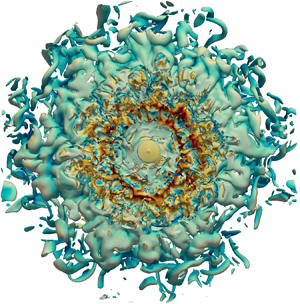
Features of the wide-open type of CVB are discussed using a typical case of  $S = 2.15$. Instantaneous features for this case are shown at an arbitrary instant in figure 8. It can be inferred from these that the flow, downstream of VB, has a large radial expansion and moves approximately parallel to the inflow plane (with
  $u_x \approx 0$), as is typical of this type of the conical form. Note that this large radial expansion leads to reduced velocity magnitudes, since the flow is now spread over a larger area, while the flow rate remains constant. It was observed that this strong radial spread leads to the flow interacting with the lateral boundaries, which can cause artificial confinement effects. However, further extending the boundary incurs a large numerical expense and hence, only the case of this swirl rate (
 $S = 2.15$) was studied for in a laterally extended domain. This is discussed in appendix B, where it is shown that most qualitative features of this type, including hysteresis behaviour, remain the same irrespective of the domain chosen. The only differences observed were that, in the extended domain, the RZ's radius is larger while its streamwise extent is reduced. Note that the characteristic features of this type of CVB are observed in the vicinity of the inflow plane, while downstream, there is negligible flow. Since the former is captured well in both domains, the smaller domain was employed at all other swirl rates examined here, so as to reduce numerical expense.

Figure 8. Instantaneous features for wide-open conical form of vortex breakdown (CVB) at  $S = 2.15$: axial velocity contours on (a)
  $z = 0$ and (b)
  $x = 2$ planes and (c) isosurfaces of vorticity magnitude (
 $|\boldsymbol {\omega }| = 0.3$). The axial velocity range shown is chosen for clarity and is smaller than the actual range.
The time-averaged features of the wide-open CVB are shown in figure 9. It is seen from the figure that the approximately conical sheet downstream of VB sharply reverses direction and moves towards the inflow plane (see region of  $r \approx 5$ and
  $1 \leq x \leq 3$) as it continues to expand radially. Indeed, the strongest flow reversal (
 $u_x < 0$) in the mean flow field is observed in this region and not in the RZ, while the fluctuating component has maximum intensity here. Note that the flow interacts with the lateral boundary, at which the projected streamlines become almost parallel to the boundary (
 $7 \leq x \leq 20$ and
  $r \approx 20$). This effect was found to be absent when the domain is extended (see appendix B). Additionally, the RZ extends almost to the streamwise boundary for the present domain which is not the case when the lateral boundaries are extended.

Figure 9. Time-averaged flow features for wide-open conical form of vortex breakdown (CVB) at  $S = 2.15$: (a) projected streamlines and contours of
  $u_x$ and (b) rms of fluctuating axial velocity on meridional plane.
4. Bistability
The turbulent flow states that are admissible for the same inflow parameters and  $Re$ are examined in this section. As alluded to previously (see figure 1b), it was observed from hysteresis studies that both the bubble and conical forms of VB are bistable forms. Similarly, the regular and wide-open types of CVB were found to be bistable. It should be clarified that the term ‘bistable’ is used here only to denote the sustenance of the two forms/types of VB for the same boundary conditions and does not refer to the stability of the flow states. Incidentally, hysteresis effects were not observed for the BVB about
  $S = S_c$. Note that Billant et al. (Reference Billant, Chomaz and Huerre1998) have reported hysteresis behaviour near the swirl threshold. It is unclear why this difference in trend exists. One possible explanation is that it is due to the differences in inflow profiles, which occur due to the converging nozzle used in their experiments (see appendix B, Moise & Mathew (Reference Moise and Mathew2019), p. 351). Features of the bistable forms/types are examined in the following sections while a hysteresis diagram is provided at the end.
4.1. Regular and wide-open types of the conical form
Projected streamlines on the meridional plane based on the time-averaged velocity fields of the regular and wide-open types of CVB at  $S = 2.1$ are compared in figure 10(a). The stark difference in the size of the RZ between the two types is evident, with the ‘eye’ of this zone positioned at
  $x \approx 5$ and
  $r \approx 4$ for the regular type, while
  $x \approx 12.5$ and
  $r \approx 14$ for the wide-open type. However, it was also observed that the flow structure upstream of VB (
 $x \approx 1$) is approximately the same for both cases. This is highlighted in figure 10(b), which shows the centreline mean axial velocity for the two types. It can be clearly seen that the differences are negligible upstream of the position of VB (i.e. the first point along the axis where
  $u_x = 0$, see inset). The differences manifest downstream, with the reverse flow relatively weaker for the wide-open type. The existence of differences only downstream of VB and the hysteresis behaviour observed suggest that the wide-open type might be sustained due to the Coanda effect. This was confirmed by examining the pressure fields and is discussed in § 6.2.3, but it is apparent from the figure that there are large differences between the two types, clearly establishing that it is useful to classify the wide-open type as distinct from the regular type of CVB, albeit closely related.

Figure 10. Comparison of time-averaged flow features for  $S = 2.1$ using (a) projected streamlines on meridional plane and (b) centreline axial velocity variation (inset showing variation in the vicinity of the stagnation point), for conical form of vortex breakdown (CVB) types: ---------, black (thick), regular; ---------, red (thin), wide-open.
4.2. Bubble and conical forms
A comparison of the bistable bubble and conical forms of VB for  $S = 1.5$ is made in figure 11. The instantaneous axial velocity contours on the
  $z = 0$ plane clearly highlight the spheroidal and conical recirculation zones of the BVB and CVB respectively. The remaining plots show the time-averaged features. The presence of a stagnation point at the RZ's nose in the time-averaged flow field for both forms can be inferred from the streamwise variation of centreline velocity plotted in figure 11(c) (see inset). The two-celled structure of the BVB and the relatively larger one-celled RZ of the CVB are compared in figure 11(d). It is instructive to compare the present turbulent case (
 $Re = 1000$) with that at the same
  $S$ in the laminar regime (cf. Moise (Reference Moise2020a), figure 3, p. 11, for
  $Re = 200$). For the latter, the recirculation zones for the CVB and BVB have a maximum radius of around 15 and 1, respectively, while in the present case, it is 6 and 2, respectively. Thus, it is seen that the differences between the two forms is considerably reduced with an increase in
  $Re$. The implications of these are further discussed in § 6.1.2. This difference between the two forms was observed to be further reduced at a lower swirl of
  $S = 1.4$, as shown in figure 12(a) (see also, movies 5 and 6 and the hysteresis diagram, figure 12b).

Figure 11. A comparison of the bistable turbulent bubble and conical forms of vortex breakdown for  $S = 1.5$. Instantaneous axial velocity contours of (a) bubble form of vortex breakdown (BVB) and (b) conical form of vortex breakdown (CVB) shown along with (c) centreline velocity (inset showing variation in the vicinity of the stagnation point) and (d) projected streamlines based on time-averaged velocity fields comparing the two forms: ---------, blue (thin), BVB; ---------, black (thick), CVB.

Figure 12. (a) Comparison of time-averaged flow features using projected streamlines on meridional plane for bistable forms at  $S = 1.4$: ---------, blue (thin), bubble form of vortex breakdown (BVB); ---------, black (thick), conical form of vortex breakdown (CVB). (b) A hysteresis curve based on maximum radial extent of a streamline starting from
  $x = 0$ and
  $r = 0.2$, both obtained as swirl rate,
  $S$, is varied for
  $Re = 1000$ (regions of overlap shaded grey): (
 $\triangle$, blue), pre-VB; (
 $\circ$, green), oscillating BVB; (
 $\times$, black), regular CVB; (
 $\square$, red), wide-open CVB.
4.3. Hysteresis diagram
A hysteresis diagram is shown in figure 12(b) based on all the stationary, sustained VB states that occur in overlapping  $S$ ranges for
  $Re = 1000$ and the inflow condition, the Maxworthy profile with
  $\alpha = 100$ and
  $\delta = 0.2$. This is based on the maximum radius,
  $\sigma _{max}$, achieved by a projected streamline starting at
  $x = 0$ and
  $r = 0.2$, computed using the mean velocity field. Note that the streamline chosen is arbitrary but represents the qualitative features of all the VB states well and
  $\sigma _{max}$ is commensurate to the RZ size. As
  $S$ is increased beyond
  $S_c = 1.14$,
  $\sigma _{max}$ associated with the BVB is seen to gradually increase (green symbols), representative of the increase in the RZ's size with swirl. By contrast, for regular CVB, the parameter remains approximately a constant for most
  $S$, except close to the threshold of
  $S = 1.4$. This indicates that the transition to turbulence limits the radial spread of the conical sheet for the regular CVB. The wide-open CVB is seen to increase in size with increasing
  $S$, although confinement effects prevent further scrutiny.
5. Coherent structures
Features of the coherent structures observed in the simulations are further scrutinized here. The power spectral density (PSD) estimate as a function of the dimensionless frequency,  $f$, is shown in figure 13(a) for different fluctuating velocity components. This is shown for time series collected at selected positions on the axis, at
  $x = 8$ and
  $6$ for cases
  $S = 1.3$ and 1.4, respectively. The estimate was computed using the Welch's method with the data divided into overlapping time intervals of 500 (overlap of 50 %) and using a Hamming window function. For the fluctuating axial velocity component,
  $u_x'$ (dashed curve), a dominant peak is present at
  $f \approx 0.01$ for
  $S = 1.3$ and at
  $f \approx 0.005$
  $S = 1.4$. By contrast, a peak in the PSD of
  $u_y'$ (solid curve) is seen at
  $f \approx 0.13$ for both swirls. The positions examined here are representative of the flow features, i.e. the maximum energy of the axisymmetric oscillation is relatively weaker for
  $S = 1.4$ at all probe positions when compared to
  $S = 1.3$ while that of the spiral mode is approximately the same. Also, it is emphasized that for both cases, the fluctuations are negligible in the vicinity of the bubble's nose, as can be inferred from figure 5(b).

Figure 13. Power spectral density estimate for the time series of (a) fluctuating velocity components for bubble form of vortex breakdown (BVB),  $u_x'$ (- - - -) and
  $u_y'$ (---------) obtained on the axis (
 $y = z= 0$) at
  $x = 8$ at
  $S = 1.3$ (black) and
  $x = 6$ for
  $S = 1.4$ (red) and (b)
  $u_y'$ for conical form of vortex breakdown (CVB) at different
  $S$ and
  $(x,y,z)$ probe locations.
Since visual examinations of the flow field revealed only axisymmetric and spiral structures of azimuthal wavenumber  $m = 0$ and
  $+1$, respectively (cf. figure 3), the results can be interpreted as follows. The velocity components
  $u_y' = u_z' = 0$ for axisymmetric modes, while
  $u_x' = 0$ for spiral modes (as can be seen by considering the symmetry of these modes about the
  $y = 0$ axis in the
  $z=0$ plane, e.g. Batchelor & Gill Reference Batchelor and Gill1962). Thus, a periodic axisymmetric motion occurs at
  $f \approx 0.01$ for
  $S = 1.3$ which is of lower energy and frequency for
  $S = 1.4$, while for both swirls, a spiral mode is present with
  $f \approx 0.13$. The relatively high energy associated with the axisymmetric oscillations at
  $S = 1.3$ which reduce for
  $S = 1.4$ can also be inferred from visual inspection of the axial velocity contours shown in movie 1 and movie 3. This also explains the relatively high fluctuating r.m.s velocity,
  $|u_x'|$, seen in
  $6 \leq x \leq 8$ and
  $r \leq 1$ for
  $S = 1.3$ in figure 5(b) which is almost twice the value seen for
  $S = 1.4$ in the same region. Examining the PSD computed at other centreline positions further confirmed this. Additionally, the PSD at positions away from the centreline, as expected, show two discernible peaks for all velocity components in the approximate region of
  $6 \leq x \leq 10$ for
  $S = 1.3$ and
  $6 \leq x \leq 8$ for
  $S = 1.4$.
For the CVB, the cases of  $S = 1.4$ and 1.5 were examined for coherent oscillations in the vicinity of where the spiral vortices were observed. The PSD estimate of the fluctuating radial velocity component at position
  $x = 6$ and
  $z = 0$ with
  $y = 5$ for
  $S = 1.4$ and
  $y = 6$ for
  $S = 1.5$ is shown in figure 13(b). There seem to be peaks at
  $f\approx 0.05$ for both cases, but these are not dominant and were absent for the other velocity components. While the vortical structures are expected to have only negligible energy content due to low velocities associated with the large radial expansion of the cone, it will be shown below that these peaks are spurious by examining the signal's time-frequency behaviour.
A continuous wavelet transform was employed to check for intermittent variations in dynamics of the spiral structures seen in the simulations. The magnitude of the transform for the fluctuating velocity,  $|W(u_y')|$, was computed using MATLAB by employing the ‘Bump’ wavelet (which has a relatively narrow variance in frequency). The corresponding scalograms are shown in figure 14 for BVB at
  $S = 1.3$ and
  $S = 1.4$. Note that the time,
  $t$ is based on the start of the simulation and the interval shown is after the initial transients till the end of simulation for each case. At both swirls, as expected, a band of high amplitude can be discerned at
  $f \approx 0.13$ for both cases. However, peaks in amplitude also appear intermittently in time for
  $f \approx 0.1$ and 0.08 for
  $S = 1.3$ and 1.4, respectively. These results indicate that the frequency of rotation of the spiral coherent structure varies intermittently in time. One possible reason for this could be the streamwise oscillations observed in the flow.

Figure 14. Scalogram showing the magnitude of the continuous wavelet transform of  $u_y'$ for
  $x = 8$ on the axis for the bubble form of vortex breakdown at (a)
  $S = 1.3$ and (b)
  $S=1.4$.
The scalogram for the time series of  $u_y'$ at
  $x = y =6$ and
  $z = 0$ is shown for CVB at
  $S = 1.5$ in figure 15(a). It is clearly seen that no specific frequency dominates in the flow field. Similar behaviour was observed in the scalograms at other location and for
  $S = 1.4$. Thus, it is concluded that although there are large-scale spiral vortical structures present in the flow field (figure 6), they do not have a coherent dynamic behaviour.

Figure 15. (a) Scalogram showing the magnitude of the continuous wavelet transform of  $u_y'$ for
  $x = y = 6$ and
  $z = 0$ for conical form of vortex breakdown (CVB) at
  $S = 1.5$. (b) Variation of the dominant eigenvalue from spectral proper orthogonal decomposition,
  $|\lambda _1(f)|$, with the frequency is shown for bubble form of vortex breakdown (BVB) at different swirls.
Next, the modal decomposition technique of SPOD (Lumley Reference Lumley1970; Picard & Delville Reference Picard and Delville2000; Towne et al. Reference Towne, Schmidt and Colonius2018) is used to examine the spiral coherent structures seen for the BVB. SPOD was carried out using data from the  $z = 0$ plane and the three-dimensional structure of the modes was inferred by examining the symmetry about the
  $y = 0$ axis. For example, the
  $y$-velocity component is expected to be antisymmetric and symmetric about the
  $y = 0$ axis for the axisymmetric and spiral modes, respectively. Note that only the higher frequency range associated with the spiral coherent structures are examined using SPOD, while the lower frequency axisymmetric oscillations seen in the PSD are not (cf. figure 13). This is due to the constraints arising from low frequency resolution and the spectral leakage associated with the reduced time interval of the blocks which are employed for better estimating the cross-spectral density.
For both  $S = 1.3$ and 1.4, only the modes associated with the dominant eigenvalue,
  $\lambda _1(f)$, were observed to contain non-negligible energy content. Variation of this eigenvalue's magnitude,
  $|\lambda _1(f)|$, with frequency is shown in figure 15(b). For
  $S = 1.3$, the spectra shows peaks with energy content spread in the band
  $0.09 \leq f \leq 0.15$, which matches with that seen in the scalogram (figure 14a). The spatial structure of the modes in this band of frequencies is similar and thus, only the dominant peak at
  $f \approx 0.12$ is considered. For
  $S = 1.4$, a dominant peak occurs at
  $f \approx 0.13$, but another subdominant peak is also observed for
  $f \approx 0.18$. However, there are no oscillations observed at any probe locations at this frequency in both the periodogram and the scalogram suggesting that it is spurious. It is unclear why this mode occurs, but it is ignored and only the dominant mode at
  $f \approx 0.13$ is considered.
For both swirls, the  $y$-velocity component for the dominant SPOD mode was found to be symmetric about the
  $z = 0$ plane indicating that it represents a spiral structure (not shown). The real part of the axial velocity component of this SPOD mode for the two swirls is shown in figure 16 for
  $y > 0$. As expected for a spiral mode, the axial velocity component is zero on the axis. As is clear from the figure, this SPOD mode is positioned relatively upstream for
  $S = 1.4$. Note that for both cases, the bubble's streamwise position is approximately
  $2 \leq x \leq 6$, implying that the mode interacts with the bubble only for
  $S = 1.4$. By contrast, the dominant SPOD mode for
  $S = 1.3$ is observed to be associated with the second RZ that is present in the near wake of the bubble. Nevertheless, the spatial structure of these SPOD modes are approximately the same for the two cases, with similar radial extent and pitch.

Figure 16. Contours of axial velocity's real part for the dominant spiral spectral proper orthogonal decomposition (SPOD) mode associated with the bubble form of vortex breakdown at (a)  $S = 1.3$ and (b)
  $S = 1.4$. Projected streamlines based on time-averaged flow field additionally plotted for reference.
In summary, the above results suggest the following. For the case of BVB at  $S = 1.3$, a spiral coherent structure of
  $m = +1$ is present in the wake of the bubble. At a higher swirl of
  $S = 1.4$, this spiral structure is positioned relatively upstream starting at the rear part of the bubble and having a larger radius, but a similar streamwise length. The positioning of this spiral could explain the loss of the second RZ downstream for
  $S = 1.4$. Note that as a linearly unstable mode grows in amplitude, the base flow can be distorted by the nonlinear interactions of the mode as it evolves towards saturation (Sipp & Lebedev Reference Sipp and Lebedev2007). Manoharan et al. (Reference Manoharan, Frederick, Clees, O'Connor and Hemchandra2020) have shown, using a weakly nonlinear analysis for a PVC, that the nonlinear interaction of the global mode with its conjugate leads to a base-flow distortion that counteracts the bubble's length. While what is observed here is not the PVC, it is possible that a similar mechanism could be involved in modifying the base flow. This speculation is also made based on somewhat similar features seen at lower
  $Re$ for laminar flow states (see base and mean flows shown in Moise (Reference Moise2020a), figure 13, p. A31–19). For the CVB, the results indicate that the spiral vortices observed do not rotate at a specific frequency.
6. Discussions
6.1. Identification of flow states
The rich variety and diversity of flow states observed in swirling flows has made the correct identification and classification of these states difficult. Further, categorization without examining the velocity field and carrying out hysteresis studies can lead to misleading results. These aspects are discussed below with the focus on the spiral and conical forms of vortex breakdown.
6.1.1. The spiral form of vortex breakdown
The flow features observed here for the BVB at  $S = 1.3$ show the presence of a spiral structure downstream to a bubble with no stagnation point at the latter's nose (§ 3.2). Since the flow is mostly laminar and axisymmetric in the bubble region, a sufficiently thin dye filament introduced along the axis at inflow would travel through it unperturbed and would take a spiral path downstream to the bubble. Thus, this dye visualization would indicate an SVB and not a BVB. At higher
  $S$, at which the stagnation point appears intermittently, the visualization would indicate spontaneous transitions between the BVB and SVB. These aspects, including the downstream position of SVB as compared to BVB and the spontaneous transitions between the two (see § 1), resemble those reported in experiments that predominantly used dye visualization to identify these two forms (Sarpkaya Reference Sarpkaya1971; Faler & Leibovich Reference Faler and Leibovich1977). Additionally, the streamwise oscillating motion observed too matches with similar observations for SVB in such experiments. Thus, the flow state at
  $S = 1.3$ might also be classified as an SVB, though such classifications that solely rely on dye visualizations are misleading and ambiguous. Further, while it has been proposed that the SVB is associated with the precession of the bubble (Brücker Reference Brücker1993; Gallaire et al. Reference Gallaire, Ruith, Meiburg, Chomaz and Huerre2006), it is speculated based on the present results, that the SVB reported in experimental studies such as Sarpkaya (Reference Sarpkaya1971) and Faler & Leibovich (Reference Faler and Leibovich1977) might be associated with the loss of stagnation point at the bubble's nose and the presence of a spiral structure downstream. However, this requires further validation. Note that for all
  $S$, the spiral is present only downstream to the bubble, which remains approximately axisymmetric. Thus, it should be emphasized that this flow state is not the PVC which is commonly observed at high
  $Re$ (Syred Reference Syred2006; Oberleithner et al. Reference Oberleithner, Sieber, Nayeri, Paschereit, Petz, Hege, Noack and Wygnanski2011; Manoharan et al. Reference Manoharan, Frederick, Clees, O'Connor and Hemchandra2020).
6.1.2. The conical form of vortex breakdown
Instantaneous flow features of the regular CVB are shown in figure 17 using axial velocity contours on the  $z= 0$ plane for
  $S = 1.4$ and 1.45. Interestingly, for
  $S = 1.4$, the RZ could easily be mistaken as that associated with a BVB. For example, in Liang & Maxworthy (Reference Liang and Maxworthy2005), a majority of the VB flow states reported closely resemble the regular CVB, although they have not identified as so. Indeed, the cases shown in figure 17 strongly resemble that shown in figure 5(b) of Liang & Maxworthy (Reference Liang and Maxworthy2005) even though the Reynolds numbers in that study is only half of the value used here. Similarly, figure 45 in Syred & Beer (Reference Syred and Beer1974), figure 7 in Gore & Ranz (Reference Gore and Ranz1964), figure 3 in Aguilar et al. (Reference Aguilar, Malanoski, Adhitya, Emerson, Acharya, Noble and Lieuwen2015), figures 4 and 5 in Tammisola & Juniper (Reference Tammisola and Juniper2016), figure C.8 in Falese et al. (Reference Falese, Gicquel and Poinsot2014), figures 3 and 4 in Jiang & Shen (Reference Jiang and Shen1994), figure 5 in Adzlan & Gotoda (Reference Adzlan and Gotoda2012) and figure 5 in Apte et al. (Reference Apte, Mahesh, Moin and Oefelein2003) show flow states with features resembling CVB, although further investigation is required to confirm if these flow states are the CVB.

Figure 17. Projected velocity vectors on  $z = 0$ plane at arbitrary instants for (a)
  $S = 1.4$ and (b)
  $S = 1.45$, showing regular conical form of vortex breakdown (CVB). These flow states closely resemble that reported in Liang & Maxworthy (Reference Liang and Maxworthy2005) (length scale changed to jet diameter, i.e.
  $x_D = x/2$, for ease in comparison).
The present results suggest that the turbulent CVB is only approximately conical when compared to the laminar CVB (Moise Reference Moise2020a), with the differences between BVB and CVB reduced here. Thus, a simple criterion using time-averaged features to distinguish the two states might become an oversimplification at higher  $Re$, although the two remain distinct flow states, as shown by the hysteresis studies. Also, while there are similarities between the two VB forms, there are also crucial differences. For example, at this
  $Re$, the BVB is seen to have a two-celled bubble for most of the swirl range (see figure 5a), while the cone of the regular CVB has a one-celled structure for all
  $S$ (see figures 10(a) and 12(a)). Similarly, the dynamical behaviour and the coherent structures associated with the two forms are different (§ 5 and animations).
Incidentally, it must be emphasized that the present results indicate that the CVB does not have an ‘open’ RZ. Both BVB and CVB have two stagnation points, one at the nose and other at the rear of the closed RZ (laminar regular CVB, cf. figure 3(c), Moise (Reference Moise2020a); turbulent regular CVB: cf. 11c). Some experiments on unconfined swirling jets seem to indicate that the RZ is open for CVB, but this is might be erroneously inferred from the limited field of view of PIV. Additionally, inferences based only on dye visualization can be misleading, since the dye's strength will be strongly reduced along  $x$ as the expanding cone's cross-sectional circumference increases with
  $x$. Another possibility is that the inferences are made for the wide-open type of CVB, in which a strong Coanda effect (see § 6.2.3) might cause an open stagnation zone.
In conclusion, while there are a handful of studies that do identify the regular CVB and distinguish it from BVB, many have not reported or identified its occurrence. Based on the results of the present study, it is postulated that this could be because CVB can be easily misidentified as a BVB and additionally, because hysteresis effects are not always examined. While the swirl generating mechanisms and thus, the inflow conditions are expected to still play a major role in the sustenance of CVB, scrutiny of the flow structure with swirl variation and performing hysteresis studies could help in better identifying CVB when it occurs. Studies at still higher  $Re$, with the flow being turbulent at inflow would be needed to understand the effect of turbulence on these two flow states, since the differences between these might play an important role in engineering applications, especially in determining mixing efficiency in combustors.
6.2. Ranges of existence
Interestingly, the BVB and regular CVB seen here exist only in finite ranges of swirls, while the wide-open type is observed only above a threshold value. These results are compared with other studies and predictions of some existing models on VB below. Additionally, a discussion on possible mechanisms for sustenance is also provided.
6.2.1. Critical swirl
The critical swirl,  $S_c$, above which VB occurs is considered first. For
  $Re = 1000$, it has been shown here that
  $S_c = 1.14$, while for
  $Re = 200$, it has been previously reported that
  $S_c = 1.39$ (Moise & Mathew Reference Moise and Mathew2019). These results suggest that the critical swirl increases when
  $Re$ reduces. With no inflow perturbations, this is not an effect of turbulence, although the transition to turbulence affects the RZ features. This trend is consistent with experimental observations (Spall, Gatski & Grosch Reference Spall, Gatski and Grosch1987) and it has been generally observed that
  $S_c$ decreases for increasing
  $Re$ and stays approximately constant above a particular
  $Re$ for laminar inflow conditions. The trend at lower
  $Re$ can be expected based on the following argument. Consider a strongly swirling flow with azimuthal and axial velocity scales of
  $u_\theta ^0$ and
  $u_x^0$ (
 $\ll u_\theta ^0$). If the latter velocity component is used as the reference scale, then the Reynolds number,
  $Re^0$, based on this will be ‘low’, while the swirl number based on these scales,
  $S^0 = u_\theta ^0/u_x^0$, would be ‘large’. Thus, in the limit of a purely rotating flow, i.e. as
  $u_x^0 \rightarrow 0$, the dimensionless parameters
  $Re^0 \rightarrow 0$ and
  $S^0 \rightarrow \infty$. Since VB is not expected to occur for such purely rotating flows, it implies that the critical swirl,
  $S_c^0 \rightarrow \infty$. This indicates that as
  $Re$ becomes very low,
  $S_c$ would start to increase.
Various estimates of  $S_c$ in the range of
  $Re$ for which it is approximately constant have been proposed previously. Billant et al. (Reference Billant, Chomaz and Huerre1998) hypothesized a necessary condition for VB, assuming a steady, axisymmetric, inviscid mechanism, given by
 \begin{equation} \int_0^\infty\frac{u^2_\theta(0,r)}{r}\textrm{d} r \leq \frac{1}{2}. \end{equation}
For  $\delta = 0.2$, this criterion gives
  $S_c = 1.078$, which is close to the observed value of 1.14 for BVB, but not that of the CVB. Another empirical estimate for determining the threshold of VB was given in Spall et al. (Reference Spall, Gatski and Grosch1987). The inflow Rossby number, defined as
  $Ro = u^*_x/(r^*\varOmega )$, was proposed as a governing parameter, where
  $r^*$ is the radius at which swirl velocity is maximum,
  $u^*_x$ is axial velocity at
  $r^*$ and
  $\varOmega$ is the rotation rate. The authors, by considering a variety of available numerical and experimental studies, showed that for large enough
  $Re$ the critical Rossby number is
  $Ro_c \approx 0.65$. Assuming here that
  $\varOmega$ is the limiting value of
  $u_\theta /r$ when
  $r\rightarrow 0$, the critical Rossby number for the Maxworthy profile, based on
  $S_c$ for
  $Re = 1000$, is
  $Ro_c = 0.99$ which is higher than their estimate. It is not clear why this is the case, although it should be noted that Spall et al. (Reference Spall, Gatski and Grosch1987) did not include any studies which examined swirling jets when arriving at the heuristic estimate for
  $S_c$.
6.2.2. Comparison to ranges in the laminar regime
Interestingly, the bubble form occurs in the range  $1.39 \leq S \leq 1.78$ for
  $Re = 200$ (Moise Reference Moise2020a), while it is observed here for
  $1.14 \leq S \leq 1.5$ suggesting that the BVB exists for approximately the same extent of swirl range at different
  $Re$, but has a lower threshold swirl at higher
  $Re$. A similar comparison for the CVB is not possible as the exact ranges for the regular and wide-open type were not determined at
  $Re = 200$ (due to the enormous radial expansion of the flow and the associated numerical expense) but it is noted that the wide-open type was observed at
  $Re = 200$ for
  $S = 2$, while here, it is seen only for
  $S \geq 2.1$. These results indicate that
  $Re$ and/or the flow regime can play an important role in the sustenance of a given flow state.
6.2.3. Mechanisms of sustenance
As alluded to in § 1, although various attempts have been made to understanding the mechanisms underlying VB, they remain limited in explaining VB's rich features and predicting its occurrence or sustenance. The BVB seems to be present for all families of swirling flows, while the CVB is reported (or inferred) only for swirling jets, suggesting that the outer shear layer might play a crucial role in the sustenance of this form. To understand these aspects and the bistability behaviour seen here, several approaches were attempted, as documented below.
The mean flow solutions of all VB flow states were examined for conical similarity (Shtern & Hussain Reference Shtern and Hussain1999), but were not found to exhibit this property. The theory of Benjamin (Reference Benjamin1962) has been shown in Moise (Reference Moise2020b) to predict an increasing RZ size when  $S$ is decreased, which is in contradiction to the present results. The inviscid theory of Wang & Rusak (Reference Wang and Rusak1997) was also examined in Moise (Reference Moise2020b) and shown to predict a stagnation zone of infinite radius when confinement effects are neglected which prevents comparisons with the present results. Another approach towards understanding bistability using nonlinear adjoint-based optimization was formulated (Moise & Mathew Reference Moise and Mathew2017; Pradeep Reference Pradeep2019) but was not pursued due to associated numerical expense and feasibility concerns. Thus, the exact mechanisms that sustain BVB and regular CVB seen here remain unexplained.
By contrast, the sustenance of the wide-open type of CVB can be explained using the phenomenon of Coanda effect. Such a mechanism has been proposed for similar flow states observed for annular swirling jets when a stepped-conical expansion is used at inflow (Vanierschot & Van den Bulck Reference Vanierschot and Van den Bulck2007). Note that in the present study, the velocity field in the coflow region of the inflow plane (approximately,  $r > 1$) is negligible (
 $u_x = 0.01$ and
  $u_y = u_z = 0$, see § 2.1) implying that it can be approximated as a wall. Thus, the Coanda effect would cause the sheet of flow that is conically expanding downstream of VB to get ‘attracted’ towards the inflow plane. This is also expected to occur at very high
  $S$ where the cone's opening angle is high and would also explain the hysteresis features observed. To check for Coanda effects, the time-averaged inflow pressure of the bistable regular and wide-open types at
  $S = 2.1$ are compared in figure 18(a). Here the freestream pressure at
  $r = 20$,
  $p_\infty$, is used as reference. In contrast to the regular CVB, the pressure is lower in the approximate region of
  $1 \leq r \leq 6$ for the wide-open type. This is where the conical sheet reverses direction and turns towards the wall as shown in figure 18(b) using meridional streamlines and mean pressure for the wide-open type. This is not the case for the regular CVB, as shown in figure 18(c). The development of a low pressure region just upstream to the region where a jet attaches to a wall is one key characteristic of the Coanda effect. To further confirm this effect, the transition from a regular to wide-open CVB was examined by changing the inflow swirl from
  $S = 2.2$ to
  $S = 2.3$ at a rate of
  $10^{-3}$ and maintaining it at the latter value (i.e. the same approach followed in the hysteresis studies). Figure 19(a) shows pressure contours on the
  $z=0$ plane at different times. At time,
  $t = 100$, when the inflow swirl reaches the
  $2.3$ which is maintained for the rest of the simulation, the CVB remains a regular type. This is still the case at
  $t = 500$, but a pressure reduction is observed for
  $4\leq r\leq 4$, approximately. At
  $t = 700$, the CVB is a wide-open type, with pressure further reduced in this region. This is better seen by examining the inflow pressure profiles at these times, which are plotted in figure 19(b). This figure further shows that a mildly lower pressure drop is present in the coflow region at
  $t = 500$ which drops further at
  $t = 700$, but with reduced radial extent for the latter. The development of this lower pressure region is followed by the sheet approximately ‘attaching’ to the
  $x = 0$ plane. This evolution can be more clearly understood by examining the animation provided as movie 12 which provides the pressure at all instants of this transition. It should be noted that the helical vortex associated with CVB (figure 6b) causes the circular low pressure regions visible in the contours in close proximity to the conical sheet. These might play a role in the attachment by complementing the Coanda effect by inducing the conical sheet to be moved towards the inflow.

Figure 18. Time-averaged pressure for bistable types of conical form of vortex breakdown (CVB) at  $S = 2.1$: (a) comparison of profiles at inflow (
 $x = 0$) as a function of radial distance of bistable states at
  $S = 2.1$; contours on the meridional plane for (b) wide-open type and (c) regular type (projected streamlines based on mean flow shown for reference and contour range reduced in extent for clarity).

Figure 19. Instantaneous pressure fields shown for the transition from regular to wide-open conical form of vortex breakdown (CVB) when inflow swirl is varied from  $S = 2.2$ to 2.3 at constant rate in the interval
  $0\leq t \leq 100$ and then sustained at
  $S = 2.3$. (a) Contours on
  $z = 0$ plane (range reduced in extent for clarity) and (b) variation of pressure at inflow (
 $x = z = 0$) at different times.
In summary, the above results for the wide-open CVB, including the development of a low pressure region and the hysteresis effect observed clearly indicate that the wide-open type is initiated and sustained by the Coanda effect. This effect can be further examined by performing simulations in which the wall region is slanted away from the streamwise direction so as to check if the sheet also changes angle, but this is beyond the scope of this study.
6.3. Effect of inflow conditions
Various experiments have noted that for sufficiently high inflow swirl strengths, the RZ associated with VB enters into the nozzle (Liang & Maxworthy Reference Liang and Maxworthy2005; Oberleithner et al. Reference Oberleithner, Paschereit, Seele and Wygnanski2012). Thus, the reliability of results presented here, which are based on imposition of steady inflow conditions, require scrutiny. The following discussion examines under what conditions the qualitative flow features discussed here are expected in experiments (see also Moise & Mathew (Reference Moise and Mathew2019), appendix A, pp. 350–351).
6.3.1. Steady inflow at low swirls
The theory proposed in Benjamin (Reference Benjamin1962) predicts that the flow should be supercritical at inflow. While there are reasons to suspect the validity of this theory (Moise Reference Moise2020b), the supercritical nature of the inflow can still be reinterpreted as equivalent to the quasi-cylindrical approximation (QCA) being valid (Reyna & Menne Reference Reyna and Menne1988). This implies that for  $S < 1.66$, the inflow is unaffected by developments downstream due to the parabolic nature of the equations associated with the QCA. Wang & Rusak (Reference Wang and Rusak1997) have confirmed this behaviour for supercritical inflow using inviscid simulations for laminar swirling flows in pipes. Oberleithner et al. (Reference Oberleithner, Paschereit, Seele and Wygnanski2012) have reported the bubble to be downstream to the nozzle when the inflow is supercritical (cf. figure 10, p. 1444).
The inflow is supercritical for  $S < 1.66$ for the Maxworthy profile (Moise & Mathew Reference Moise and Mathew2019), which strongly indicates the reliability of the present results (bistability of BVB and CVB) in this swirl range. Further, as discussed above in § 6.1.2, the VB state reported in Liang & Maxworthy (Reference Liang and Maxworthy2005) strongly resembles the CVB seen here. Additionally, bistability of BVB and CVB is indicated by the spontaneous transitions between these states reported in Billant et al. (Reference Billant, Chomaz and Huerre1998).
6.3.2. Effect of nozzle geometry
Experiments usually employ a nozzle downstream of the swirl-generating equipment as a passage for the swirling jet as it enters into the region of study. Nozzle geometry can play an important role in the type of mode selected. For example, if the nozzle is long relative to its diameter, then the BVB seems to be preferred (e.g. Oberleithner et al. (Reference Oberleithner, Sieber, Nayeri, Paschereit, Petz, Hege, Noack and Wygnanski2011):  $L_n/D = 600/51\approx 11.8$, where
  $L_n$ is nozzle length and D is jet diameter; Manoharan et al. (Reference Manoharan, Frederick, Clees, O'Connor and Hemchandra2020):
  $L_n/D \approx 6.92/2.54 \approx 2.7$) while the CVB seems to be preferred for short nozzles (Billant et al. (Reference Billant, Chomaz and Huerre1998):
  $L_n/D = 9.2/8.5 \approx 1.1$; Liang & Maxworthy (Reference Liang and Maxworthy2005):
  $L_n/D = 2.5/1.5 \approx 1.7$). This could be explained as follows.
VB has been reported to always occur downstream of the swirl-generating equipment in Gore & Ranz (Reference Gore and Ranz1964). Denoting the streamwise position of VB as measured from the generating equipment when no nozzle is employed as  $x_0 > 0$, it is possible that when a stationary nozzle of length
  $L_n$ is used, VB would occur within it if
  $x_0 < L_n$. This is possible under the assumption that the spatially thickening boundary layer at the nozzle wall does not strongly affect the flow. For CVB, the confinement associated with a nozzle of length
  $L_n \gg x_0$ might prevent the conical expansion. Further, the nozzle shape would also play a role. Indeed, CVB seems to be present when conically-expanding nozzles are employed (cf. figure 45, Syred & Beer (Reference Syred and Beer1974) and figures 7(h) and 7(i) in Vanierschot & Van den Bulck Reference Vanierschot and Van den Bulck2007). Thus, the present results would be representative of experiments where a sufficiently short nozzle is used such that VB does not enter into it.
6.3.3. Steady inflow at high swirls
At higher swirls ( $S \geq 1.66$), the validity of the results (existence of wide-open CVB and its bistability with regular type) need to be interpreted with caution. As mentioned above, if the nozzle remains short, the CVB might be preferred. Further, the wide-open type can be inferred to occur mainly in two studies: Gore & Ranz (Reference Gore and Ranz1964) and Mourtazin & Cohen (Reference Mourtazin and Cohen2007). In the former, this type is observed at highest swirls studied when no nozzle is used. The latter used a nozzle which was also rotated implying that the nozzle also causes swirl generation. These observations suggest that CVB and wide-open CVB observed here at high
  $S$ would be representative of what would happen when the nozzle is absent/short/rotating. Nevertheless, it is emphasized that this requires further experimental confirmation.
7. Conclusions
Motivated by the rich and varied features of VB flow states observed for unconfined swirling jets in the laminar regime (Moise & Mathew Reference Moise and Mathew2019; Moise Reference Moise2020a), the present study examines features of VB for such flows at a relatively higher Reynolds number value at which it is accompanied by a transition to turbulence. For this purpose, large eddy simulations were performed with the Maxworthy profile employed as the inflow condition (§ 2). This profile models a steady, laminar, axisymmetric swirling jet and is dependent on three parameters, of which the swirl rate,  $S$, alone is varied in this study. The length and velocity scales are the jet radius and centreline velocity, respectively and the Reynolds number based on these was fixed at
  $Re = 1000$.
Although artificial disturbances were not added at the inflow, a transition to turbulence was observed for all cases studied. For streamwise-invariant initial conditions, the pre-VB swelling, BVB, regular CVB and wide-open CVB occur, in that order, with increasing  $S$ (§ 3). This sequence is similar to that observed for
  $Re=200$ at which the flow remains laminar (Moise & Mathew Reference Moise and Mathew2019). Similarly, the ranges of
  $S$ in which these states occur could be further extended by means of hysteresis studies (§ 4). Thus, it is shown that a transition to turbulence does not affect bistability features.
Periodic stagnation point formation and flow reversal associated with a BVB were observed at a critical swirl of  $S_c = 1.14$. However, presence of possibly spurious structures prevented scrutiny of the BVB features in the swirl range
  $1.14 \leq S \leq 1.2$. The BVB was examined in detail in the swirl range
  $1.3 \leq S \leq 1.5$ (§ 3.2) where the structures are absent. For
  $S =1.3$ and 1.4, strong streamwise oscillations occur and the core jet flow penetrates through the bubble, implying that the RZ is toroidal. Additionally, a spiral coherent structure of azimuthal wavenumber
  $m = +1$ (counter-winding and co-rotating) was identified in the wake of the bubble and was further examined using spectral proper orthogonal decomposition (§ 5). For
  $S = 1.3$, the spiral structure develops downstream of the bubble, while at higher swirls, it develops relatively upstream. Based on the toroidal RZ observed for
  $S = 1.3$ and the intermittent appearance of a stagnation point at higher
  $S$, it is speculated that the spiral form of VB reported in previous studies might occur due to the loss of stagnation point at the bubble's nose (§ 6.1.1).
The regular and wide-open types of CVB occur in the swirl ranges of  $1.4 \leq S \leq 2.2$ and
  $S \geq 2.1$, respectively. The lateral extent of the RZ associated with regular CVB is significantly smaller in comparison to the extent attained when the flow remains laminar (Moise & Mathew Reference Moise and Mathew2019). The wide-open type has a relatively enormous RZ compared to the other VB states, with a maximum radius of approximately 20 jet radius, as compared to 6 and 2 associated with regular CVB and BVB, respectively. The development of low pressure regions where the radially-expanding flow turns towards the inflow plane shows that the sustenance of the wide-open type is due to the Coanda effect.
Through hysteresis studies, it is shown here that the turbulent BVB and regular CVB are bistable forms (§ 4.2, figure 11). Similarly, it is established that the regular and wide-open types are bistable (§ 4.1, figure 10). The differences in length scales associated with the bistable turbulent BVB and CVB are relatively smaller when compared to their laminar counterparts. The flow features of the bistable regular and wide-open types of CVB are the same upstream of breakdown, but starkly different downstream.
An important conclusion from the present study is that the reduced differences between the bubble and conical forms in the turbulent regime and their bistability can lead to misidentification of the regular CVB as a BVB (§ 6.1.2). Further, the coexistence of several VB states, as shown here and in Moise (Reference Moise2020a), indicates that results of studies on swirling flows might be misleading if hysteresis studies are not performed. For example, the results from this study strongly suggest that many of the flow states reported in Liang & Maxworthy (Reference Liang and Maxworthy2005) and several other studies are actually the CVB. The differences in the RZ's spatial structure and the spiral vortical structures of the BVB and CVB highlighted here show that these states have distinct characteristics. Thus, correctly identifying the underlying VB flow state might be potentially useful in engineering applications, including in improving combustor designs. In this regard, further investigations examining the effects of confinement, temperature variation, inflow conditions and Reynolds number on the features and bistability of these VB forms are required for better differentiating between the two and further generalizing the results of this study.
Supplementary movies
Supplementary movies are available at https://doi.org/10.1017/jfm.2021.118.
Acknowledgements
We thank R. Rayan for help with the numerical code. All simulations were performed using SahasraT, a Cray XC40 supercomputer at the Supercomputer Education and Research Centre (SERC), Indian Institute of Science, Bengaluru. We also thank the reviewers for insightful comments which helped improve this study.
Declaration of interests
The authors report no conflict of interest.
Appendix A. Onset of VB
As noted above, the presence of  $|m|=4$ structures for
  $S\leq 1.2$ prevents making conclusive inferences from the simulation results at VB onset. Thus, only a brief account of the features observed for swirls close to
  $S_c = 1.14$ are documented here. The time-averaged flow fields are shown in figure 20 for
  $S = 1.13$, 1.14 and 1.15 using projected streamlines overlaid on axial velocity contours on the meridional plane. The kink seen for the radially outermost streamline is because of the
  $|m|=4$ structure. The time-averaged centreline axial velocity component for the three cases are compared in figure 21(a).

Figure 20. Time-averaged features of flow states close to vortex breakdown (VB) onset shown using projected streamlines and axial velocity contours on the meridional plane for (a)  $S = 1.13$, (b)
  $S_c = 1.14$ and (c)
  $S = 1.15$. Note that only
  $x \geq 5$ is shown for clarity.

Figure 21. (a) Time-averaged centreline axial velocity and (b) periodogram of the fluctuating axial velocity component at  $x = 7$ on the axis.
At  $S = 1.13$, although flow reversal was observed in the instantaneous flow field, no stagnation point is present in the time-averaged velocity field. Instead, only a ‘swelling’ is seen in figure 20(a), similar to that seen at low
  $Re$ (Moise & Mathew Reference Moise and Mathew2019). At
  $S = S_c = 1.14$, a one-celled BVB (see § 1) is seen, with two stagnation points present on the axis (figure 21a). What appears to be a two-celled BVB is seen in the mean flow for the case of
  $S = 1.15$, with four stagnation points present on the axis, but the
  $|m|=4$ structure has a strong influence on the flow field for this case. There are similarities between this sequence of mean flow states observed here in this swirl range (swelling, followed by one-celled BVB, followed by two-celled BVB, with increasing
  $S$) and those reported for
  $Re = 200$.
Interestingly, coherent periodic oscillations were observed in the flow field for the cases of  $S = 1.13$ and
  $S_c = 1.14$, but were absent for
  $S = 1.15$. This can be inferred from the periodogram showing the estimate of power spectral density (PSD) of the fluctuating axial velocity component compared in 21(b) for the three swirls. The PSD is based on the time series collected at a position of
  $x = 7$ on the axis (
 $y = z= 0$). A dominant peak is present for both
  $S = 1.13$ and 1.14 at a dimensionless frequency,
  $f_0 \approx 0.02$ (scaled based on inflow centreline axial velocity and jet radius). These results suggest that the bubble develops and disintegrates in a periodic fashion in the flow field for the lower swirls before being permanently present for
  $S = 1.15$. This is supported by results from Vanierschot & Ogus (Reference Vanierschot and Ogus2019) on transitional annular swirling jets. In their study the authors have shown by extracting coherent flow structures that similar oscillations occur due to the periodic appearance of the bubble at the onset of VB, with a Strouhal number based on the inner diameter to be
  $St \approx 0.02$. This has not been pursued here, since the
  $|m|=4$ structures are expected to exert a strong influence on the flow structure.
Appendix B. Simulations of wide-open CVB in a larger domain
For the case of turbulent wide-open CVB discussed in § 3.3.2, the conical sheet expanded radially to an extent almost equal to the lateral dimensions of the domain ( $L_y = L_z = 40$). Thus, an investigation on the effect of domain dimensions on this flow state was carried out by simulating the same (
 $S = 2.15$ and
  $Re = 1000$) in a laterally extended domain of
  $L_y = L_z = 80$, while retaining
  $L_x = 40$. The instantaneous flow features are shown in figures 22(a) and 22(b) (see also movie 11). Note that the sheet's maximum radius is approximately 30, which is lower than the radial extent of the extended domain. The time-averaged flow features using projected streamlines on a meridional plane are shown in figure 22(c). The time-averaging was carried out for a time of
  $t \approx 680$ only, due to numerical expense. However, since no temporal variations of large time-scales could be detected, this is assumed adequate. For the mean flow, it is seen that the sheet extends up to
  $r = 25$, which cannot be captured using the domain used in the rest of this study (
 $L_y = L_z = 40$). This seems to introduce some differences between the results obtained here and those for the previous domain (cf. figure 9). In the latter case, the sheet, after the initial radial expansion towards the later boundary, remained almost parallel to the streamwise direction for approximately
  $10 \leq x \leq 20$, and the RZ extended close to the outflow boundary (
 $x = 40$). For the present case, the sheet gradually curved (
 $x = 15$,
  $r = 25$), similar to a regular CVB, with the volume of the RZ limited to
  $x = 25$. However, the two characteristic features – the large-scale axisymmetric radial expansion of a conical sheet and the reorienting of this sheet towards the inflow plane beyond a particular distance – are both captured well in both domains.

Figure 22. Flow features for case  $S = 2.15$ and
  $Re = 1000$ simulated in a larger domain of
  $L_y = L_z = 80$ and
  $L_x = 40$: instantaneous axial velocity contours on (a)
  $z= 0$ and (b)
  $x = 2$ planes, and (c) time-averaged features shown using projected streamlines based on mean velocity field. The axial velocity range shown is chosen for clarity and is smaller than the actual range.
Bistability of the wide-open type with regular CVB was also confirmed by sustaining the former in the larger domain for  $S = 2.1$. The wide-open type was observed till the end of simulation (
 $t = 3980$, not shown), with the lateral spread of the sheet remaining much less than the extent of the lateral boundaries. Since the lateral extent of the smaller domain is more than sufficient for regular CVB at this
  $S$ (see figure 10), the results indicate that the wide-open and regular types are bistable irrespective of confinement effects.


 Open access