


1. Introduction
The natural world is filled with shapes formed by a process involving either melting or dissolution accompanied by fluid flow (Ristroph Reference Ristroph2018). Examples include the dissolution of a lump of sugar in water, the melting of an ice cube, the melting of icebergs, glaciers and ice shelves (Hewitt Reference Hewitt2020), the shaping of caves and rock spires (Meakin & Jamtveit Reference Meakin and Jamtveit2010) and the karstification of subsurface salt deposits (which can lead to catastrophic land subsidence and sinkholes, e.g. Frumkin & Raz Reference Frumkin and Raz2001). The coupling between fluid flow and the evolution of solid boundaries driven by melting, dissolving or eroding processes create a rich variety of free-boundary problems in which the evolution of the surface forms part of the problem to be determined. A classical example is the Stefan problem in which the evolution of a melting solid is coupled to thermal diffusion (e.g. Jaeger & Carslaw Reference Jaeger and Carslaw1959). However, in many common examples, the flux of heat or solute across the interface between the ambient fluid and the body results in a buoyancy-driven convective flow along the surface that controls the flux. There remains a fundamental open question with regard to the shapes that arise as a consequence of this two-way interplay between the evolution of geometry and the dynamics of buoyancy-driven convective flow.
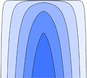
In this study, we address this problem in situations where the convective flow is driven by buoyancy directed towards the surface of the body, retaining a gravitationally stable flow (figure 1). In the preceding paper (Pegler & Davies Wykes Reference Pegler and Davies Wykes2020), we developed a new model describing the evolution of the shape of a body in this regime (to be reviewed in § 2) given by a single partial differential equation describing the evolution of the surface of the body. The predictions of the model were found to be in excellent agreement with the results of a series of laboratory experiments involving the dissolution of upwards-pointing cones of sugar candy attached to the base of a water-filled tank. Both the descent of the tip and the full shape of the evolving body over time were captured successfully by the theory with no use of any adjustable parameters.

Figure 1. Schematics illustrating (a) the general configuration, (b) an example of a shallow geometry ( $h_x \ll 1$) and (c) a steep geometry (
 $h_x \gg 1$).
Our mathematical analysis of the model in Pegler & Davies Wykes (Reference Pegler and Davies Wykes2020) focused on the illustrative example in which the body is initially wedge shaped or conic. For this specific initial condition, similarity solutions provide exact solutions to the model applicable for all times. In this case, the tip of the body descends as  $t^{4/5}$ and the curvature of the tip decreases as
  $t^{-4/5}$, where
  $t$ is time. If the initial shape is not wedge shaped or conic, a single similarity solution of this kind is not available. The result is a considerably richer variety of phenomena and transitional similarity solutions, which we explore here.
The aim of the present paper is to identify, investigate and elucidate these new phenomena. We conduct a complete analysis of the shape evolutions resulting from general nonlinear initial shapes, using power laws as a template, thereby encompassing shapes initialised with rectangular profiles to those that start with a sharp tip. The analysis identifies all fundamental similarity solutions to the model, and shows that these solutions describe the shape of a dissolving or melting body during the evolution at small or large times. We demonstrate that the initial shape determines the asymptotic shapes and scalings of the tip position for all time, while the tip assumes a universal shape structure. For the first time, it is established that a dissolving or melting tip can either blunt or sharpen, or even switch from blunting to sharpening during the evolution, depending on the initial shape.
In essence, the model of Pegler & Davies Wykes (Reference Pegler and Davies Wykes2020) generalises classical theories of stable thermal or solutal convection along surfaces to account for the evolution of the underlying surface. Classical experimental and theoretical work (Wagner Reference Wagner1949; Merk & Prins Reference Merk and Prins1953; Ostrach Reference Ostrach1953) have determined that the thermal or solutal flux produced through dissolution, heating or cooling along a vertical or sloped wall of constant inclination is proportional to  $s^{-1/4}$, where
  $s$ is the distance from the top of the wall, a result predicted by a similarity solution to the governing boundary-layer equations. The flux decreases with distance along the wall because accumulation of solute acts to insulate the dissolving surface from the fresh ambient fluid as the boundary layer grows downstream. The analysis of buoyancy-driven boundary layers has since been extended to numerous generalisations, including two-component compositional convection involving both heat and solute diffusion (Josberger & Martin Reference Josberger and Martin1981; Wells & Worster Reference Wells and Worster2011). Owing to a favourable property of the governing boundary-layer equations, the self-similar structure with flux decreasing as
  $s^{-1/4}$ is preserved in this and numerous other generalisations. This includes general dependences of the viscosity, diffusivity or density on the solute or temperature field of the fluid (Pegler & Davies Wykes Reference Pegler and Davies Wykes2020). The shaping predicted by the model of Pegler & Davies Wykes (Reference Pegler and Davies Wykes2020) therefore correspondingly applies to a broad range of applications. Consequently, the shapes arising during the dissolution of rock candy in water (where the viscosity varies by orders of magnitude) are similar to those arsing during the melting of a floating ice cube in salty water, which can include two-component effects such as latent heating.
Previous research into the inverted case where the buoyancy is directed away from the surface (e.g. the underside of a block of ice melting in warm water, or a suspended block of rock candy dissolving in fresh water), has shown that the evolution develops a uniform and constant mean recession rate of the solid surface controlled by the dynamics of unstable free convection. This relatively simple model can explain the evolution of the general shape of the base of a melting or dissolving body (Mcleod, Riley & Sparks Reference Mcleod, Riley and Sparks1996; Davies Wykes et al. Reference Davies Wykes, Huang, Hajjar and Ristroph2018; Cohen et al. Reference Cohen, Berhanu, Derr and Courrech du Pont2020) or the roof of a dissolving cavity (Gechter et al. Reference Gechter, Huggenberger, Ackerer and Waber2008). Other work has considered melting, dissolving or eroding bodies submerged in an externally forced flow (Hao & Tao Reference Hao and Tao2001, Reference Hao and Tao2002; Ristroph et al. Reference Ristroph, Moore, Childress, Shelley and Zhang2012; Moore et al. Reference Moore, Ristroph, Childress, Zhang and Shelley2013; Huang, Moore & Ristroph Reference Huang, Moore and Ristroph2015; Moore Reference Moore2017). Oltéan, Golfier & Bus (Reference Oltéan, Golfier and Bus2013) used experiments and numerical simulations to show that, when fluid is pumped upwards through a vertical salt cavity, the morphology of the fissure depends on whether the flow is dominated by buoyancy-driven or forced convection. The analysis of shape change of a melting or dissolving object in the case of gravitationally stable natural convection has to date focused on experimental analysis (Schenk & Schenkels Reference Schenk and Schenkels1968; Vanier & Tien Reference Vanier and Tien1970; Nakouzi, Goldstein & Steinbock Reference Nakouzi, Goldstein and Steinbock2015; Davies Wykes et al. Reference Davies Wykes, Huang, Hajjar and Ristroph2018), or has neglected shape change when modelling the rate of recession (Mcleod et al. Reference Mcleod, Riley and Sparks1996).
We begin in § 2 by reviewing the development of our theoretical model. This is followed by the derivation of a new intrinsic time scale introduced by an initial condition of a general power-law form. A suite of numerical solutions to our dimensionless model is then presented to illustrate the transient evolutions that arise for a variety of initial shapes, bridging rectangular cross-sections to spiked bodies. In § 3, these regimes are analysed to reveal similarity solutions that describe the leading-order shape at early and late times. A universal regime diagram is constructed showing the transitions of the rate of descent of the tip and its sharpness. In § 4, we discuss the implications of more general initial shapes including piecewise power laws and terraced structures, the stability of the similarity solutions to perturbations and the role of thermal conduction. We end in § 5 by summarising our key conclusions.
2. Model review, intrinsic scales and illustration of evolving forms
We consider a two-dimensional body that is either melting or dissolving into an ambient fluid, forming a gravitationally stable convective flow along the surface of the body (figure 1). We assume that the fluid is Newtonian and remains laminar. Let  $(x,z)$ denote the horizontal and vertical coordinates, let
  $t$ denote time, let
  $z=h(x,t)$ denote the interface between the solid and the fluid, let
  $\alpha (x,t)$ denote the slope of the surface at a given position
  $x$ and let
  $s$ denote the arc length from the tip of the body, defined by
 \begin{equation} s_x = \sqrt{1+h_x^2}, \end{equation}
where we have used a subscript to denote the partial derivative. The rate of recession of the boundary normal to the surface,  $V$, is, for either a melting or dissolving body, assumed to be related linearly to the thermal or solutal flux according to
 \begin{equation} V = \left\{ \begin{array}{@{}ll} R \, q_C & \textrm{(dissolving)}, \\ (1/ \rho_s l) q_T & \textrm{(melting)}, \end{array} \right. \end{equation}
where  $q_C =- \kappa \partial C / \partial y$ and
  $q_T = k \partial T / \partial y$ are the solute mass flux and thermal energy flux at the surface,
  $C$ and
  $T$ are the mass concentration and temperature fields of the fluid and
  $\kappa$ and
  $k$ are the solutal diffusivity and thermal conductivity, respectively. For the case of dissolution, we define the mass concentration
  $C$ by
 \begin{equation} \rho = \rho_l + (\rho_s - \rho_l) C, \end{equation}
where  $\rho _s$ and
  $\rho _l$ are the densities of pure solid and liquid, respectively, such that
  $C=0$ represents pure solvent and
  $C=1$ pure solid. The parameter
  $R \equiv 1/ (1 - C_i)$, where
  $C_i$ is the mass concentration of the fluid at the interface. With this specification, (2.2) represents the balance between the flux of concentration released by recession of the surface,
  $V(1-C_i)$, and the flux due to diffusion away from the surface,
  $q_C$. For melting, (2.2) represents the Stefan condition, where
  $l$ is the specific latent heat. For this case, we have assumed here that the heat supplied to the surface is purely latent, i.e. that no heat is necessary to warm the body to the melt temperature before melting initiates. This assumption is applicable if the body is initialised close to the melting temperature. A detailed discussion of the conditions necessary for this assumption to apply, as well as the implications of its relaxation, are provided later in § 4.3. To ease the exposition, we henceforth assume the notation and terminology applicable to a dissolving body and drop the subscript
  $C$ from
  $q_C$ until § 4.3, where we focus specifically on melting. If the flux profile along the surface,
  $q$, were known then the recession rate
  $V$ can be determined using (2.2) and the height profile evolved forwards using
 \begin{equation} h_t ={-}s_x V, \end{equation}
where the factor  $s_x$ converts the normal rate of recession
  $V$ into the vertical rate of recession. To develop a closed model describing the evolution of the height profile
  $h(x,t)$, it therefore remains to relate the flux
  $q$ along the body to
  $h(x,t)$ at any given time.
In principle, the thermal flux along the body can be determined using the system of equations describing a solutal boundary layer. Let  $u(s,y,t)$ and
  $v(s,y,t)$ denote the tangential and normal components of the velocity of the flow, and let
  $C$ denote the mass concentration of the solution. The boundary-layer equations of the flow read
 \begin{gather} \frac{\partial u}{\partial s} + \frac{\partial v}{\partial y} = 0, \end{gather}
 \begin{gather}\rho \left( u \frac{\partial u}{\partial s} + v \frac{\partial u}{\partial y} \right) = \frac{\partial }{\partial y}\left( \mu \frac{\partial u}{\partial y} \right) + {\rm \Delta} \rho_s g \sin[\alpha(s,t)] C, \end{gather}
 \begin{gather}u \frac{\partial C}{\partial s} + v \frac{\partial C}{\partial y} = \frac{\partial }{\partial y} \left( \kappa \frac{\partial C}{\partial y} \right), \end{gather}
where  $\rho$ is the density of the fluid,
  $\mu$ is the dynamic viscosity,
  $g$ is the acceleration due to gravity and
  ${\rm \Delta} \rho _s$ is the density difference between the solid and the fluid with minimum concentration (e.g. Schlichting & Gersten Reference Schlichting and Gersten2017). These equations represent the conservation of fluid mass, momentum and solute mass, respectively. In writing these equations, we have neglected the contributions to the material derivatives due to the rates of change in time,
  $\partial u / \partial t$ and
  $\partial C / \partial t$, such that the flow can be treated as quasi-steady compared to the relatively slower time dependence of the shape evolution. As discussed in Pegler & Davies Wykes (Reference Pegler and Davies Wykes2020), the strength of this assumption can be measured using the dimensionless number given by
 \begin{equation} \varGamma = u/V, \end{equation}
representing the ratio of the flow speed to the recession speed. The limit  $\varGamma \gg 1$ corresponds to situations where the body is gradually sculpted by a relatively faster boundary-layer flow and the adjustment time of the boundary-layer system towards a quasi-steady state can be assumed to be instantaneous to good approximation.
In principle, it would be sufficient to solve the complete system of quasi-steady boundary-layer equations given by (2.5)–(2.7) subject to suitable boundary conditions (for example, a Dirichlet condition on the concentration at the interface, and suitable no-slip and far-field stagnancy conditions) in order to determine the required flux along the surface,  $q = -\kappa \partial C / \partial y$, and couple this to (2.4). However, if the Schmidt number,
  $Sc = \nu / \kappa$ where
  $\nu = \mu /\rho$, is sufficiently large (greater than unity is sufficient) then an analytical result for the flux is available that bypasses the need to solve these equations explicitly. In this limit, the solutal sublayer through which the solute concentration transitions from the ambient value to the interfacial value is considerably smaller than the viscous sublayer in which viscous stresses become important. The inertial term given by the left-hand side of (2.6) can therefore be neglected in the solutal sublayer. Under this simplification, a transformation of the boundary-layer equations is available that yields the explicit expression relating the flux along the surface of the body to any given height profile
 \begin{equation} q = {\displaystyle \frac{\displaystyle D |\sin \alpha |^{1/3} }{\displaystyle \left( \int_0^s \left|\sin \alpha \right|^{1/3} \, \textrm{d} s \right) ^{1/4} }}, \end{equation}
where  $D$ is a constant, and the local angle of inclination
  $\alpha$ can be related to the height profile
  $h(x,t)$ by
  $\sin \alpha = -h_x/s_x$. This result is derived by Acrivos (Reference Acrivos1960). A step-by-step derivation is provided in Pegler & Davies Wykes (Reference Pegler and Davies Wykes2020), where it is noted in particular that the result generalises to situations in which the viscosity, diffusivity or density can all be specified as any given function of either temperature or solute concentration. For a dissolving body,
  $D \equiv \gamma \kappa _i C_i ({\rm \Delta} \rho _s g C_i/\kappa _{\infty } \mu _\infty )^{1/4}$, where the
  $i$ subscripts denote quantities in the fluid evaluated at the interface, and the
  $\infty$ subscripts denote quantities evaluated in the far field (the analogue expression for
  $D$ for melting is provided in Appendix C.1). The dimensionless prefactor
  $\gamma$ encapsulates any functional dependences of viscosity and diffusivity on concentration (the value
  $\gamma \approx 0.5027$ applies for uniform properties). For the case of an instantaneously uniform
  $\alpha$, (2.9) reduces to
  $q \propto s^{-1/4}$, recovering the prediction of the similarity solution arising for a constant surface slope (Wagner Reference Wagner1949; Merk & Prins Reference Merk and Prins1953; Ostrach Reference Ostrach1953).
Using (2.9) and (2.2) to evaluate  $V$ in (2.4) and using the identity
  $\sin \alpha = -h_x / s_x$, we obtain the governing equation for the surface evolution
  $h(x,t)$ given by
 \begin{equation} h_t = {\displaystyle \frac{\displaystyle - A |h_x s_x^2|^{1/3} }{\displaystyle \left( \int_0^x |h_x s_x^2 |^{1/3} \, \textrm{d} x \right) ^{1/4} }}, \end{equation}
where  $s_x^2 = h_x^2 + 1$, first derived in Pegler & Davies Wykes (Reference Pegler and Davies Wykes2020). This integro-differential hyperbolic equation independently describes the evolution of the surface of a melting or dissolving body subject to an initial condition on
  $h(x,0)$. For dissolving bodies, the parameter
  $A \equiv R D$ is associated purely with the material properties of the fluid and the solid under consideration. The parameter can be interpreted as the prefactor in the profile of the recession rate that would apply for the case of a vertical wall,
  $V = As^{-1/4}$. Since
  $A$ can be absorbed directly into the time
  $t$, it follows that the shapes that arise for a given initial condition are universal, with
  $A$ controlling only the speed at which the dissolution and shape transitions take place.
2.1. Similarity solutions for initial wedges and cones
In Pegler & Davies Wykes (Reference Pegler and Davies Wykes2020), we considered the preliminary example of initially wedge-shaped bodies defined by  $h(x,0) = -m|x|$, where
  $m$ is a positive constant representing the initial slope of the sides. This produces a unique situation where (2.10) admits exact similarity solutions that apply for all time of the form
 \begin{equation} h(x,t) = (At)^{4/5} f \left( \frac{x}{(At)^{4/5}} \right), \end{equation}
where  $f$ is the shape function determined from the similarity analysis (dependent on the parameter
  $m$). The shape profile predicted by (2.11) ‘stretches’ as
  $t^{4/5}$ in both the vertical and horizontal dimensions, such that the distance between the tip and its initial position increases as
  $h_0(t) = f_0 t^{4/5}$, where
  $f_ 0 \equiv f(0)$ is the tip-descent prefactor. The prefactor was found to be given asymptotically by
  $f_0 \sim -1.49\, m^{2/5}$ in the limit of shallow slopes (
 $m \to 0$) and by
  $f_0 \sim -1.30\, m^{4/5}$ in the limit of steep slopes (
 $m \to \infty$). The solution demonstrates in particular that the information of the initial position of the tip is preserved in the evolution for all times. A further feature, indicated by the scaling for the curvature of the tip,
  $h_{xx} \sim h/x^2 \sim (At)^{-4/5}$, is that the tip blunts with time. Identical scalings apply to cones derived from an analogue axisymmetric theory, but with slightly modified prefactors (
 $\,f_0 \sim -1.726 \, m^{2/5}$ as
  $m \to 0$ and
  $f_0 \sim -1.505\, m^{4/5}$ as
  $m \to \infty$). By conducting a series of laboratory experiments, we showed that the model not only predicts the descent rate correctly with no adjustable parameters, but also the entire shape profile, thereby validating the general model. As we will show here, more general (nonlinear) initial conditions result in a considerably richer variety of new similarly solutions and asymptotic transitions, including the potential for both sharpening and blunting of the tip.
2.2. Tip shape and the relationship between tip curvature and descent rate
Before considering solutions to the model above, we review a selection of results from Pegler & Davies Wykes (Reference Pegler and Davies Wykes2020) concerning the admissible shape near the tip and the relationship between the descent speed of the tip and the local tip curvature that follow immediately from (2.10). By considering possible forms of the asymptotic shape,  $h \sim x^{\alpha }$ for
  $x \to 0$ in the right-hand side of (2.10), we find that this equation reduces to
 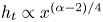 $h_t \propto x^{(\alpha -2)/4}$. Therefore,
  $\alpha =2$ is the only value for which the descent speed of the tip
  $h_t$ is finite. A tip moving at a finite speed must therefore be parabolic, i.e.
 \begin{equation} h(x,t) \sim h_0(t) - \tfrac{1}{2} S(t) x^2, \end{equation}
as  $x \to 0$, where
  $h_0(t) \equiv h(0,t)$ is the tip height and
  $S(t) \equiv |h_{xx}(0,t)|$ is the tip curvature or sharpness. Shapes that are initialised at
  $t=0$ with a non-parabolic tip will either remain instantaneously stationary at
  $t=0$ if
  $\alpha > 2$, or move instantaneously with infinite speed if
  $\alpha < 2$ (with an integrable singularity, meaning that the tip position remains finite). In either case, the tip will immediately transition to being parabolic for all times
  $t>0$ with the curvature of the tip either increasing from zero if
  $\alpha > 2$ or decreasing from infinity if
  $\alpha < 2$ (a property that will be confirmed by our later analyses). In both cases, the instantaneous evolution of the tip shape is such as to regularise the dissolution profile of a free-convective boundary layer by forming the unique shape for which the bounday layer produces a locally smooth dissolution rate at the tip (Pegler & Davies Wykes Reference Pegler and Davies Wykes2020).
It should be noted that, while the shape near a dissolving tip is therefore universally parabolic, the broader tip profile is generally better represented by a different, non-parabolic form. For example, initially steep bodies generally produce a much larger region in which a  $4/3$-power shape applies in an intermediate asymptotic region near the tip, with the parabolic region confined to an asymptotic sublayer that can be many orders of magnitude smaller (see Pegler & Davies Wykes Reference Pegler and Davies Wykes2020, and § 3.2.1 here). It should also be noted that, very close to the tip, a generalised boundary-layer model that includes contributions due to gradients in hydrostatic pressure may play some role as the tip surface becomes horizontal near the tip (a regime that applies to thermal or solutal boundary layers on horizontal substrates). A discussion of this is provided in appendix B of Pegler & Davies Wykes (Reference Pegler and Davies Wykes2020).
Substituting (2.12) into (2.10), we determined further that the speed of descent of the tip satisfies
 \begin{equation} \frac{\textrm{d} h_0}{\textrm{d} t} ={-}A\left( \frac{4}{3} S(t) \right)^{1/4}, \end{equation}
yielding a general law relating tip-descent speed and tip sharpness (for axisymmetric bodies, the prefactor is 16 % larger; Pegler & Davies Wykes Reference Pegler and Davies Wykes2020). Sharper tips therefore descend faster, at a rate proportional to the tip curvature  $S(t)$ to the
  $1/4$ power. With the parameter
  $A$ known, the result of (2.13) allows the curvature of a dissolving tip to be determined from measurement of the descent speed alone, thereby bypassing the need for direct measurement of the tip curvature at the microscale.
2.3. Intrinsic scales and non-dimensionalisation
As a template for illustrating the variety of transitional behaviours and asymptotic regimes that apply to freely melting or dissolving bodies, we allow here for a general class of initial shapes of the power-law form
 \begin{equation} h(x,0) = h_0(x) ={-}L^{1-n} |x| ^n, \end{equation}
where  $L$ is a length scale and
  $n$ is a positive exponent defining the initial shape. This specification allows for initially rectangular cross-sectioned bodies (
 $n = \infty$), convex parabolae (
 $n=2$), triangular peaks (
 $n=1$) and concave inverse parabolae (
 $n=1/2$). For
  $n \neq 1$, the length
  $L$ represents the horizontal scale of the shape. For example,
  $2L$ is the width of the rectangle for
  $n=\infty$, and the radius of curvature of the parabola for
  $n=2$. For
  $n=1$, (2.14) reduces to
  $-|x|$ and, in this special case, the length scale
  $L$ is lost from the problem. Consequently, there is a unique degeneracy in the specification for
  $n=1$ that requires a dimensionless initial slope
  $m$ to be specified for generality (Pegler & Davies Wykes Reference Pegler and Davies Wykes2020). In this case, the lack of any intrinsic length scale in the problem results in similarity solutions that apply for all time. The existence of the intrinsic length scale
  $L$ for
  $n \neq 1$ precludes a single similarity solution from applying for all time, with the result of producing more complex transitions.
For  $n \neq 1$, (2.10) and (2.14) yield the scalings of
  $h/t \sim (h/x)^{1/4}$ and
  $h \sim x \sim L$, respectively. Combining these scales, we derive the intrinsic time scale in the problem,
 \begin{equation} T = L^{5/4} / A. \end{equation}
With a suitable multiplicative prefactor, this time scale represents the time taken for the surface of a melting or dissolving body to recede a characteristic distance  $L$. For example,
  $\beta T$ characterises the time scale for a cylinder of material of diameter
  $2L$ and height L to melt in a quiescent environment, where
  $\beta$ is an order-one dimensionless prefactor specific to this shape. For a length scale of
  $L = 1 \ {\rm cm}$, we evaluate
  $T \approx 110$ min using the value
  $A \approx 1.5 \times 10^{-4}$ cm
 $^{5/4}$ s
 $^{-1}$ measured for candy dissolving in water (Pegler & Davies Wykes Reference Pegler and Davies Wykes2020). The scaling in (2.15) implies that a body ten times larger in side length would take
  $10^{5/4} \approx 18$ times longer to melt. As we will show, the unique intrinsic time
  $T$ also represents the time scale on which the shape transitions between different asymptotic self-similar regimes.
We non-dimensionalise the model of (2.10) by defining the non-dimensional variables, denoted by hats, according to
 \begin{equation} x = L \hat{x}, \quad s = L \hat{s}, \quad h = L \hat{h}, \quad t = T \hat{t}. \end{equation}
On dropping hats, (2.10) and (2.1) become
 \begin{equation} h_t = {\displaystyle \frac{\displaystyle - |h_x s_x^2|^{1/3} }{\displaystyle \left( \int_0^x \left|h_x s_x^2 \right|^{1/3} \, \textrm{d} x \right) ^{1/4} }}, \quad s_x = \sqrt{1+h_x^2}, \end{equation}
respectively, and the initial condition (2.14) becomes
 \begin{equation} \quad h(x,0) ={-}|x|^n. \end{equation}
The initial shape exponent  $n$ provides the only parameter in the dimensionless system above. Thus, the transient forms of freely dissolving and melting bodies of any power-law shape can be determined following a systematic exploration of the solutions to the dimensionless system above over
  $n$.
$n$.
2.4. Overview of predicted shape evolutions
As an overview of the possible general evolutions, we begin by illustrating a suite of numerical solutions to (2.17a,b) and (2.18) for various values of  $n$. For this, we employed the second-order upwind finite-difference scheme detailed in Pegler & Davies Wykes (Reference Pegler and Davies Wykes2020). The evolutions of the profiles calculated for
  $n=100$, 2, 1, and
  $0.5$ are shown in panels (a)–(d), respectively. In each case, the profile is shown at a progression of times,
  $t = 0, 1, \ldots 5$. The right-hand plots show the corresponding evolutions of the tip position
  $h_0(t)$ as red curves. The overlaid lines of circles and dashes represent asymptotic predictions (with appropriate dimensionless prefactors) that will be determined later in the analyses of § 3.
The case  $n=100$ shown in panel (a) of figure 2 is representative of the limiting case of an initially rectangular body,
  $n=\infty$. The numerical solution shows that the initial effect of dissolution is to round the corners of the rectangle. At early times, the large majority of the dissolution occurs along the near-vertical edges of the body, producing a progressively taller aspect ratio. By
  $t\approx 2$, the initially blunt tip has formed a sharp needle-like profile. The tip subsequently descends at a much faster rate. The plot of the descent distance of the tip in the right-hand panel illustrates a relatively sudden acceleration of the descent rate for
  $t \gtrsim 2$. The descent position switches from a scaling of
  $t^{4/3}$ at early times to the considerably faster scaling of
  $t^4$ at late times. The evolution of the tip sharpness
  $S(t)$ plotted in figure 3(a) shows a correspondingly abrupt increase in the rate of sharpening from a
  $t^{4/3}$ trend at early times to a very fast
  $t^{12}$ trend at late times.

Figure 2. A suite of numerical solutions to the dimensionless model (2.17a,b)–(2.18) for (a) a near-rectangular initial profile,  $n=100$, (b) a parabolic initial profile,
  $n=2$, (c) a piecewise linear initial profile,
  $n=1$, and (d) an inverse parabolic initial profile,
  $n=0.5$. The left-hand plots show the evolution of the shape
  $h(x,t)$ at a progression of dimensionless times
  $t=0, 1, 2, 3, 4$ and 5 (the last is not visible in (a)). On the right, we show as red curves the evolution of the tip-descent distance,
  $|h_0(t)| = |h(0,t)|$, illustrating transitions between the shallow theory of § 3.1 and the steep theory of § 3.2. The predictions of the similarity solutions under the shallow theory are overlaid by a line of black hollow circles, while those of the steep theory are overlaid as dashed black lines. For cases (a,b), the transition switches from the shallow regime to the steep regime. For case (c), there is a similarity solution given by (2.11) in which the shape scales in both the vertical and horizontal dimensions as
  $t^{4/5}$ with respect to the starting level of the tip
  $z=0$ (Pegler & Davies Wykes Reference Pegler and Davies Wykes2020). For case (d), the shape transitions away from a steep regime at early times to a shallow regime at late times, representing a reversal of the regime progressions compared to (a) and (b).

Figure 3. The evolution of the tip sharpness,  $S(t) = |h_{xx}(0,t)|$, as a function of time for initial shape exponents of (a)
  $n=100$, (b)
  $n=2$ and (c)
  $n=1$, derived from the numerical solutions of figure 2. The plots illustrate the potential for melting or dissolving objects either to sharpen or blunt with time, the precise conditions for which are analysed in § 3.1. The asymptotic predictions of (3.9) and (3.18) are shown as lines of circles and dashes, respectively. Case (a) illustrates a pronounced transition to a rapid
  $t^{12}$ growth in the tip curvature for
  $t \gtrsim 5$. Case (c) illustrates progressive blunting of the tip as
  $t^{-4/5}$, corresponding to the prediction of the special similarity solution that applies for
  $n=1$ given by (2.11) for
  $m=1$.
The solution arising for an initially parabolic shape ( $n=2$) is illustrated in figure 2(b). Initially, the shape descends at a near-uniform rate, forming a regime in which the surface retains its full parabolic shape at early times. This contrasts to the case
  $n=100$ discussed above, where the early-time recession of the surface was primarily horizontal. For
  $t \gtrsim 1$, the profile transitions to a more pointed shape with a sharper tip. A qualitatively similar, if less extreme, asymptotic transition from an initially smooth tip to a sharper tip occurs as compared to the case
  $n=100$ above. Likewise, the tip descends faster at larger times. In this case, the tip position descends as
  $t$ at early times and at the faster rate of
  $t^{4/3}$ at late times. The evolution of the sharpness
  $S(t)$ plotted in figure 3(b) shows that the tip sharpens for all time, initially with a slow rate of sharpening from the initial value
  $S(0) = 2$ and transitioning towards the faster rate of
  $S \sim t^{4/3}$.
For the case  $n=1$ shown in figure 2(c), the initial recession speed is largest in the locale of the tip, contrasting with the behaviour of the two cases
  $n=2$ and 100 discussed above. In further contrast, the initially sharp tip rounds out, and continues to blunt for all time. In this case, figure 3(c) shows that the sharpness indeed decreases with time as
  $S(t) \sim t^{-4/5}$, implying that the tip blunts with time. This behaviour contrasts qualitatively with the two cases
  $n=100$ and 2 discussed above, for which the tip sharpens for all time. The results thus demonstrate that the tips of dissolving objects can either blunt or sharpen depending on their initial shape.
Figure 2(d) shows the case  $n=1/2$, providing an example of an initially concave shape with a spiked tip. In this case, the transience represents a reversal of the order of the regime transitions that apply to the cases of (a,b) above. Instead of transitioning from a shallow tip to a steeper tip, the profile transitions from an initially steep tip to a shallower tip. The right-hand plot of panel (d) shows a transition from a steep regime descending as
  $t^{1/3}$ at early times to a shallow regime descending as
  $t^{4/7}$ at long times. This reversal illustrates the possibility for the slopes of the surface of a melting body either to steepen or shallow with time, and the dependence of which of these occurs on the initial shape.
3. Asymptotic solutions and regime transitions
The suite of solutions above demonstrated transitions between two different asymptotic regimes. The two limits represent distinct asymptotic reductions of the model: one arising in situations where the surface in the locale of the tip is near horizontal ( $h_x \ll 1$), referred to as the shallow regime, and the other arising in situations where the surfaces in the locale of the tip are nearly vertical (
 $h_x \gg 1$), referred to as the steep regime.
3.1. Shallow theory
If the slope of the body is shallow, the theory can be simplified under the approximation that the along-slope component of gravity is determined to leading order by the local slope. That is,  $s_x \approx 1$ and the relationship
  $\sin [\alpha (x,t)] \approx -h_x / s_x$ simplifies to
 \begin{equation} \sin[\alpha(x,t)] \approx{-}h_x, \end{equation}
and (2.17a,b) and the initial condition reduce to
 \begin{equation} h_t = {\displaystyle \frac{\displaystyle - |h_x |^{1/3} }{\displaystyle \left( \int_0^x |h_x |^{1/3} \, \textrm{d} x \right)^{1/4} }}, \quad h(x,0) ={-}|x|^{n}, \end{equation}
forming a shallow-slope limiting form of the theory (Pegler & Davies Wykes Reference Pegler and Davies Wykes2020). With this reduction, it is now impossible to form an intrinsic horizontal length scale in the problem without incorporation of time  $t$, indicating the existence of similarity solutions. By considering the scalings in (3.2a,b), the relevant similarity coordinate
  $\xi$ and shape function
  $f(\xi )$ can be determined as
 \begin{equation} x = t^{{4}/{(3n + 2)}} \xi, \quad h = t^{{4n}/{(3n + 2)}} f(\xi), \end{equation}
respectively. In accordance with (3.3b), the tip descends as
 \begin{equation} h_0(t) = f_0 t^{4n/(3n+2)}, \end{equation}
where  $f_0$ is an unknown dimensionless prefactor dependent on the initial-slope exponent
  $n$. For
  $n=\infty$,
  $2$,
$2$,  $1$ and
  $0.5$, the exponents in the tip-descent law (3.4) are
  $4/3, 1, 4/5$ and
  $4/7$, respectively. These results verify the tip-descent exponents indicated earlier by our numerical solutions of figure 2, occurring at early times for both cases (a)
  $n=100$ and (b)
  $n=2$, at all times for case (c)
  $n=1$ and at late times for case (d)
  $n=0.5$.
The differing role of the shallow regime as a late-time asymptotic solution if  $n<1$ but as an early-time asymptotic solution if
  $n>1$ can be understood by considering the limits of time (
 $t \to 0$ or
  $t \to \infty$) for which the similarity scalings (3.3a,b) predict shallowing of the slope
  $h_x$. In accordance with (3.3a,b), the slope scales as
 \begin{equation} h_x \propto t^{4(n-1)/(3n+2)}. \end{equation}
Thus, the approximation of shallowness,  $h_x \ll 1$, is self-consistent as an early-time asymptote (
 $t \to 0$) only if
  $n>1$, in agreement with our numerical results of figure 2. Conversely, it provides a self-consistent late-time asymptote (
 $t \to \infty$) only if
  $n<1$.
To determine the shapes of the similarity solutions, we recast (3.2a,b) in terms of the similarity variables (3.3a,b), yielding the ordinary integro-differential system
 \begin{gather} \frac{4}{3n + 2} ( n\, f - \xi f' ) ={-} |\,f'|^{1/3} \left( \int_0^{\xi} |\,f'(\zeta)|^{1/3} \, \textrm{d} \zeta \right)^{{-}1/4}, \end{gather}
 \begin{gather}f(\infty) \sim{-}\xi^{n}. \end{gather}
The far-field condition (3.7) can be interpreted as the initial condition (2.14) recast in terms of the similarity variables (noting that  $\xi \to \infty$ as
  $t \to 0$). Alternatively, it follows from the fact that the shape in the far field (
 $\xi \to \infty$) must be given by the initial prescribed shape. This is because the boundary layer becomes fully insulating as its thickness continues to increase in the limit
  $\xi \to \infty$.
We solved the system above numerically using a shooting method in which the similarity coordinate of the tip position,  $f_0 = f(0)$, is treated as a shooting parameter. For a given trial value of
  $f_0$, we integrate (3.6) forwards from
  $\xi = 0$ to a large far-field value of
  $\xi _\infty$ using an initial-value integrator. In view of the fact that (3.6) cannot be rearranged explicitly for
  $f'$, the forwards marching was conducted using the implicit MATLAB solver ode15i. The value of
  $f(\xi _\infty )$ is then compared with the required far-field value
  $-\xi _{\infty }^n$ given by (3.7), and the value of
  $f_0$ tuned with successive iterations using the bisection method.
The resulting solutions are illustrated in figure 4. As shown in panel (b), the magnitude of the prefactor  $|\,f_0|$ increases to a maximum at
  $n \approx 0.5$ and decreases towards the asymptotic value
  $f_0 \approx -0.735$ as
  $n \to \infty$. The profiles of the solutions for
  $n=0.5$, 1, 2 and
  $\infty$ are shown in panels (c)–(f), respectively. The solution for
  $n=0.5$ inflects to a rounded tip, as shown by the enlargement in the inset of panel (c). This inflection is necessary in order for the solution to match to the parabolic form of the tip in accordance with (2.12).

Figure 4. Shallow theory predictions for the similarity solutions (§ 3.1). Panel (a) shows the exponent  $\gamma = 4n/(3n+2)$ predicted by the tip-descent law (3.4) as a function of the shape exponent
  $n$, illustrating an increase in the rate of growth as
  $n$ is increased. Panel (b) shows the corresponding magnitude of the tip-descent prefactor
  $|\,f_0|$ in (3.4) determined by solving (3.6) numerically. Panels (c)–( f) show the associated shapes of the similarity solutions for
  $n=0.5, 1, 2$ and
  $100$. The case (e)
  $n=2$ is described by the exact analytical solution (3.8), representing a parabola that descends at constant dimensionless speed
  $|\,f_0|$. An enlargement in the inset of panel (c) shows the inflection of the shape to a rounded, parabolic tip, in accordance with the general property that the tip is locally parabolic (2.12).
For an initially parabolic body,  $n=2$, (3.2a,b) admits the exact analytical solution
 \begin{equation} f = f_0 - \xi^2, \quad \textrm{where } f_0 ={-}(8/3)^{1/4}. \end{equation}
In this case, the dissolution rate over the surface of the body is uniform and the profile simply descends at a constant speed, preserving its shape. This occurs uniquely for  $n=2$ because the parabola is the special shape for which a free-convective boundary layer produces a uniform dissolution rate under the approximation of a shallow slope
  $h_x \ll 1$ assumed here.
An interesting property of melting or dissolving bodies indicated by our numerical solutions in figure 3 is their potential to either sharpen or blunt with time. Using the similarity variables (3.3a,b) to evaluate the sharpness  $S(t) = |h_{xx}(0,t)|$, we obtain
 \begin{equation} S(t) = \frac{3}{4} \left( \frac{4n|\,f_0|}{3n+2} \right)^{4} t^{4(n-2)/(3n+2)}, \end{equation}
where  $f_0$ is the descent prefactor (determined already, shown in figure 4b). We note that the exponent changes sign at
  $n=2$. Thus, cases of
  $n<2$ blunt with time and those of
  $n>2$ sharpen with time, while the case
  $n=2$ neither sharpens nor blunts, in agreement with the analytical solution of (3.8). It should be noted that the condition for blunting (
 $n < 2$) verses sharpening (
 $n > 2$) differs from the condition for shallowing (
 $n < 1$) versus steepening (
 $n > 1$). This is possible because sharpness is associated with the second derivative of the profile,
  $h_{xx}$, while steepness is associated with the first derivative,
  $h_x$, resulting in different scalings. It should also be noted that the prediction for the sharpness given by (3.9) is only applicable under the shallow regime (
 $h_x \ll 1$). A different prediction for the evolution of sharpness applies in the opposite limit of a steep body (§ 3.2), including a different critical value separating cases that blunt versus those that sharpen (
 $n=4/3$). The implication is a rich variety of scalings for the tip sharpness as a function of time, to be discussed in § 3.4.
3.2. Steep theory
A different reduction of the governing equations (2.17a,b) arises in the limit of steep slopes,  $h_x \gg 1$. In this limit, the slope is nearly vertical (
 $\alpha \approx {\rm \pi}/2$) and hence the proportion of gravity acting tangential to the slope can be approximated as
 \begin{equation} \sin[\alpha(x,t)] \approx 1. \end{equation}
The relative strength of gravity is therefore independent of the surface profile at leading order. Moreover, the arc length per unit horizontal position (2.1) can be approximated by the slope,  $s_x \approx -h_x$. The system of (2.17a,b) and (2.14) therefore simplifies to
 \begin{equation} h_t = \frac{- | h_x|}{( h_0(t) - h )^{1/4}}, \quad h(0,t) ={-}|x|^n, \end{equation}
producing a steep version of the theory. In this limit, the leading-order dissolution profile along the body corresponds to that predicted by a thermal boundary layer along an effectively vertical wall of finite height with its top at  $z = h_0(t)$.
Similarly to the shallow theory of § 3.1, the asymptotic reduction of the full model to (3.11a,b) removes the intrinsic horizontal length scale from the problem. Again, this indicates the existence of similarity solutions. By considering the scalings of (3.11a,b), we determine the relevant similarity variable  $\eta$ and shape function
  $g(\eta )$ defined by
 \begin{equation} x = t^{{4}/{(n + 4)}} \eta, \quad h = t^{{4n}/{(n + 4)}} g(\eta), \end{equation}
respectively. Thus, the tip descends as  $h_0(t) = g_0 t^{4n/(n+4)}$, where
  $g_0$ is the unknown tip-descent prefactor. Recasting (3.11a,b) in terms of (3.12a,b), we obtain the similarity system
 \begin{gather} \frac{4}{n+4} (n g - \eta g') = g' (g_0 - g)^{{-}1/4}, \end{gather}
 \begin{gather}g(\infty) \sim{-}\eta^n. \end{gather}
The system admits the analytical solution (Appendix A) given by
 \begin{equation} \frac{4n|g_0|^{1/4}}{n+4} \eta = \left(\frac{g(\eta)}{g_0}\right)^{{1}/{n}} \int_{1}^{{g(\eta)}/{g_0}} \frac{\chi^{-(n+1)/n} }{(\chi - 1 )^{1/4} } \, \textrm{d} \chi.\end{equation}
Taking the limit  $\eta \to \infty$ and imposing (3.14), we obtain the tip-descent prefactor
 \begin{equation} g_0 ={-} \left( \frac{ (n+4)\varGamma\left({\displaystyle \frac{3}{4}}\right) \varGamma \left( \dfrac{n+4}{4n} \right) }{ 4n \varGamma \left( \dfrac{n+1}{n} \right) } \right)^{{4n}/({n+4})}, \end{equation}
where  $\varGamma (x) \equiv \int _0^{\infty } \eta ^{x-1} \textrm {e}^{-\eta } \, \textrm {d} \eta$ is the gamma function. The tip-descent prefactor given by (3.16) is illustrated in panel (b) of figure 5. The values of
  $g_0$ lie between unity and the large-
 $n$ asymptote
  $g_0 \to {\rm \pi}^2/64 \approx 1.522$. The analytical solution for the shape (3.15) is shown for a selection of
  $n=0.5, 1, 2$ and
  $100$ in panels (c)–( f).

Figure 5. Steep theory predictions for the similarity solutions (§ 3.2). Panel (a) shows the exponent  $\gamma = 4n/(n+4)$ predicted by the tip-descent law (3.4). Panel (b) shows the tip-descent prefactor given by the analytical solution (3.16). Panels (c)–( f) show the shape function for
  $n=0.5, 1, 2$ and
  $100$, as predicted by the analytical solution (3.15).
For  $n=4/3$, (3.15) and (3.16) reduce to the exact power-law solution
 \begin{equation} g = g_0 - \eta^{4/3}, \quad \textrm{where } g_0 ={-}4/3. \end{equation}
Mathematically, this is the steep theory analogue of (3.8). The special case  $n=4/3$ is the critical value for which the vertical rate of recession along a buoyancy-driven boundary layer is uniform under the limit of steep slopes. The value differs from the result applicable in the shallow limit (
 $n=2$) because the simplification of the along-slope component of buoyancy differs in the two limits (it is
  $s_x \approx -h_x$, instead of
  $s_x \approx 1$). The critical value
  $n=4/3$ likewise corresponds to the special case for which the corresponding reduced theory predicts that the full shape simply descends at a constant speed (the tip descent exponent
  $4n/(n+4)$ is again unity) and retains its initial shape.
Substituting the self-similar prediction for the tip position (3.12b) into (2.13) and rearranging for the tip sharpness  $S(t)$, we obtain
 \begin{equation} S(t) = \frac{3}{4} \left( \frac{4n|g_0|}{n+4} \right)^{4} t^{4(3n-4)/(n+4)}, \end{equation}
yielding an explicit expression describing the evolution of the tip sharpness in the steep regime. The result predicts tip-descent exponents of  $-4/5$,
  $4/3$ and
  $12$ for
  $n=1, 2$ and
  $\infty$, respectively, in agreement with the numerically predicted evolutions of the sharpness at late times shown in figure 3. According to the steep regime, the shape sharpens if
  $n>4/3$ but blunts if
  $n< 4/3$, differing from the conditions predicted by the analogous result of the shallow theory (3.9). The result above confirms that the critical value
  $n=4/3$ corresponds to the case where the shape is preserved over time and neither blunts nor sharpens.
Near the tip ( $\eta \to 0$), (3.15) simplifies to the leading-order asymptotic form
 \begin{equation} g \sim g_0 - \left( \frac{3n|g_0|}{n+4} \eta \right)^{{4}/{3}} \quad (\eta \to 0). \end{equation}
Under the steep-slope approximation, the near-tip region therefore has a  $4/3$-power shape. This appears to contradict the requirement that the local tip shape is parabolic with a finite curvature
  $S(t)$, as predicted by (2.12). This conflict occurs because the approximation of steepness
  $(h_x \gg 1)$ breaks down close to the tip, where
  $h_x \to 0$. Indeed the steep solution (3.19) itself predicts that
  $g_\eta \to 0$ as
  $\eta \to 0$, thus predicting its own inconsistency near the tip. A similar asymptotic structure was also found to occur in the context of an initially conic body (Pegler & Davies Wykes Reference Pegler and Davies Wykes2020). To determine the asymptotic structure of the near-tip region, we introduced a non-steep asymptotic sublayer a distance of order
  $m^{-16/5}$ from the tip, where
  $m$ is the initial slope of the body. For power laws with
  $n \neq 1$, a similar asymptotic structure arises, except the small parameter in the problem
  $\varepsilon (t)$ is here based on time (
 $t \to 0$ if
  $n<1$ or
  $t \to \infty$ if
  $n>1$) instead of the slope scale
  $m$, as we detail below.
3.2.1. Matching the steep solution to a non-steep asymptotic sublayer near the tip
In order to reconcile the conflict between the outer steep regime and the tip, we must introduce a non-steep asymptotic sublayer that matches the inner limit of (3.19) to the parabolic solution (2.12). Following the general approach of Pegler & Davies Wykes (Reference Pegler and Davies Wykes2020), we first recast the full, unsimplified system (2.17a,b) in terms of the similarity variables derived for the steep theory (3.12a,b), and then consider the length scale on which the neglected terms intervene in the limit  $\eta \to 0$. The essential asymptotic structure is similar to that arising for wedges and cones (Pegler & Davies Wykes Reference Pegler and Davies Wykes2020), but differs in that the downstream tip shape is here a general nonlinear power law (
 $n \neq 1$) and the asymptotic parameter is now based on time
  $t$ instead of the initial slope
  $m$.
$m$.
When recast in terms of the similarity variables (3.12a,b), (2.17a,b) becomes
 \begin{equation} \frac{4}{n+4} (ng - \eta g_{\eta} ) = {\displaystyle \frac{\displaystyle -|g_\eta (\varepsilon + g_\eta^2)|^{1/3}}{\displaystyle \left[ \int_0^{\eta} |g_\eta (\varepsilon + g_\eta^2 )|^{1/3} \, \textrm{d} \eta \right]^{1/4}}}, \end{equation}
where  $\varepsilon (t) = t^{-8(n-1)/(n+4)}$ is a small time-based asymptotic parameter. The limit
  $\varepsilon \to 0$ is consistent with the property that the steep regime arises at late times for
  $n>1$ and at early times for
  $n<1$. The new terms compared to the steep theory of (3.11a,b) are represented by the
  $\varepsilon$ terms, which incorporate the slope dependence of the along-slope component of gravity. By substituting the leading-order form of the steep analytical solution in the limit
  $\eta \to 0$ given by (3.19) into (3.20) and considering the size of
  $\eta$ at which
  $\varepsilon$ becomes significant (where
  $g_\eta ^2 \sim \varepsilon$), we determine the extent of the inner region
  $\delta$ to be
 \begin{equation} \eta \sim \delta \equiv \varepsilon^{3/2} = t^{{-}12(n-1)/(n+4)}. \end{equation}
Combining this with the scaling  $g_\eta ^2 \sim \varepsilon$, we determine the associated vertical scale of the inner region as
  $g \sim \varepsilon ^{1/2} \delta \sim \varepsilon ^2$. Thus, appropriate inner variables
  $\zeta$ and
  $\psi$ can be defined by
 \begin{equation} \eta = \varepsilon^{3/2} \zeta, \quad g(\eta) = g_0 + \varepsilon^2 \psi(\zeta), \end{equation}
where  $\psi (\zeta )$ is of order unity in the non-steep sublayer. Recasting (3.20) in terms of these variables and neglecting higher-order terms, we derive the leading-order equation describing the shape through the non-steep region,
 \begin{equation} \frac{4ng_0}{n+4} = {\displaystyle \frac{\displaystyle -|\psi' (1 + \psi'^2)|^{1/3}}{\displaystyle \left[ \int_0^{\eta} |\psi' (1 + \psi'^2 )|^{1/3} \, \textrm{d} \zeta \right]^{1/4}}}. \end{equation}
This equation successfully matches the inner limit of (3.19) to a parabola near the tip with sharpness given by (3.18). To check this, we note that in the limit  $\zeta \to 0$, the terms involving the square of the slope,
  $\psi '^2$, can be neglected in (3.23). The resulting simplified equation admits the parabolic solution
  $\psi = -(\varSigma /2)\zeta ^2$ where
  $\varSigma = (3/4)(4n|g_0|/(n+4))^4$, thus recovering the required parabolic solution with sharpness (3.18). Conversely, for
  $\zeta \to \infty$, we can neglect the two instances of
  $1$ in (3.23) compared to
  $\psi '^2$. The
  $4/3$-power shape given by (3.19) provides the solution to the resulting reduced form of (3.23).
In summary, the tip of a steep body forms a double-decked structure: an inner layer of size 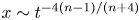 $x \sim t^{-4(n-1)/(n+4)}$ that connects the initial shape profile to the
  $4/3$-power shape given by (3.19). Closer to the tip, an inner–inner region of size
 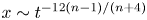 $x \sim t^{-12(n-1)/(n+4)}$ connects the
  $4/3$ shape to a deeper parabola. The inner–inner region is a factor
  $t^{-8(n-1)/(n+4)}$ smaller than the inner. For an initially rectangular body (
 $n=\infty$), this factor is
  $t^{-8}$, implying a rapid reduction in the region in which a parabola applies compared to the 4/3-power shape. The 4/3-power shape therefore dominates the larger-scale form of the shape near the tip at late times, but the tip retains a parabolic form at the finest scale.
3.3. Regime transitions
The numerical solutions in figure 2 illustrated transitions between two distinct asymptotic regimes for each case of  $n \neq 1$. Sections 3.1 and 3.2 developed asymptotic similarity solutions associated with these regimes. Here, we illustrate these transitions together in a universal parameter–time regime diagram in which the times at which the shallow or steep self-similar regimes apply to good approximation are demarcated (figure 6). To do this, we define the times,
  $t_{1}$ and
  $t_{2}$, at which the tip predicted by the full model lies within a factor of
  $1 \pm \varepsilon$ of the shallow and steep similarity solutions, respectively, where
  $\varepsilon$ is a small parameter taken as
  $0.05$. We define the transition times by
 \begin{equation} \frac{|\,f_0 t_{1}^{\lambda_1} - h_0(t_{1})|}{h_0(t_{1})} = \varepsilon, \quad \frac{|g_0 t_2^{\lambda_2} - h_0(t_2)|}{h_0(t_2)}= \varepsilon, \end{equation}
where 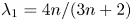 $\lambda _1 = 4n/(3n+2)$ is the tip-descent exponent associated with the shallow similarity solution (3.3a,b),
 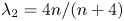 $\lambda _2 = 4n/(n+4)$ is the tip-descent exponent associated with the steep similarity solution (3.12a,b) and
  $h_0(t)$ is the tip position predicted by our numerical solution. The transition times
  $t_1$ and
  $t_2$ are plotted as functions of the shape exponent
  $n$ in figure 6. Regions of blue shading represent times at which the tip is predicted by the shallow theory, green shading represents times at which the tip is predicted by the steep theory and yellow shading represents the transitory state. For
  $n<1$, the evolution begins in the steep regime and transitions relatively quickly to the intermediate regime. The transition times diverge at
  $n=1$ because the evolution never approaches the shallow or steep asymptotic regimes in this special case, for which the distinct similarity solution of (2.11) applies exactly for all times. For
  $n> 1$, the evolutions begin in the shallow regime and transition to the steep regime. For large
  $n \gtrsim 10$, the shallow regime transitions to the steep regime with only a very brief intermission. This abrupt transition is in agreement with our numerical solutions for
  $n=100$ illustrated earlier in figure 2(a), showing that the asymptotic solutions describe the large majority of the evolution.

Figure 6. Regime diagram illustrating when the shallow and steep asymptotic regimes apply over time as a function of the initial shape exponent  $n$. The diagram is constructed by evaluating the transition times,
  $t_1$ and
  $t_2$, defined by (3.24a,b) as the times at which the numerically determined position of the tip of the body is within 5 % of the shallow and steep similarity solutions, respectively. The plot shows the transition between the shallow similarity solution (blue shading) and the steep similarity solution (green shading), and the opposite order of the regimes depending on whether the initial shape is concave (
 $n<1$) or convex (
 $n>1$). The yellow region represents times during which the evolution is transitioning from one regime to another or evolves according to the different similarity theory represented by (2.11), as applies uniquely for
  $n=1$ (indicated by the vertical dashed line). Panel (a) shows the numerical solution (black solid curve) for the illustrative example
  $n=5$ at an early time
  $t=0.05 < t_1$ for which the shallow similarity solution determined from the analysis of § 3.1 (blue dashed curve) applies to good approximation. The position of this case is indicated by a filled black circle in the regime diagram. The initial shape is indicated by a thinner grey curve. Panel (b) shows a corresponding late time
  $t = 5 > t_2$ overlaid with the steep similarity solution determined in § 3.2.
3.4. Sharpening or blunting?
The evolutions of the tip sharpnesses shown in figure 3 for  $n=100, 2$ and 1 illustrated the possibility for a dissolving or melting object either to sharpen or blunt with time, depending on its initial shape. According to the differing predictions of the shallow and steep similarity solutions, (3.9) and (3.18), the sharpness evolves in proportion to
 \begin{equation} S(t) \propto \left\{ \begin{array}{@{}ll} t^{4(n-2)/(3n+2)} \equiv t^{\sigma_1} & \textrm{(shallow)} , \\ t^{4(3n - 4)/(n+4)} \equiv t^{\sigma_2} & \textrm{(steep)}, \end{array} \right. \end{equation}
where  $\sigma _1$ and
  $\sigma _2$ are referred to as the tip-sharpening exponents in the shallow and steep regimes, respectively. If a tip-sharpening exponent is positive,
  $\sigma _i > 0$, then the corresponding similarity solution (
 $i = 1$ or 2), predicts sharpening. If the exponent is negative,
  $\sigma _i < 0$, the solution predicts blunting. To visualise the values of
  $n$ for which the tip-sharpening exponents
  $\sigma _1$ and
  $\sigma _2$ change sign, we have plotted these functions of
  $n$ in figure 7. Under the shallow regime, the tip sharpens if
  $n>2$, and blunts if
  $n<2$. On the other hand, the steep similarity solution sharpens if
  $n > 4/3$ and blunts if
  $n<4/3$. Since the order in which the shallow and steep regimes arise chronologically is based on a different condition altogether, dependent on whether
  $n<1$ or
  $n>1$, a variety of different tip-sharpening scalings are possible.

Figure 7. Tip-sharpening exponents,  $\sigma _1$ and
  $\sigma _2$, representing the powers in the evolution of the sharpening,
  $S(t) \propto t^{\sigma _i}$, for the shallow (
 $i=1$) (blue) and steep (
 $i=2$) (green) asymptotic regimes, as summarised by (3.25) and to the right of the figure above. If
  $\sigma _i > 0$, then the tip sharpens under the corresponding regime
  $i$, and if
  $\sigma _i < 0$ then the tip blunts under that regime. For
  $n<1$, the steep regime occurs at early times and the shallow regime occurs at late times. For
  $n>1$, the order is reversed. The thick branch of each curve represents the situations for which the exponent applies at early times, while the thin solid branch represents the situations for which it applies as late times. For case A (
 $n < 1$), both
  $\sigma _1<0$ and
  $\sigma _2<0$ and hence the tip blunts for all times. For case B (
 $1 < n < 4/3$),
  $\sigma _1<0$ and
  $\sigma _2<0$ again, implying blunting for all times. However, the temporal order in which exponents apply is reversed compared to case A. For case C (
 $4/3 < n < 2$),
  $\sigma _1<0$ but
  $\sigma _2>0$, implying that the tip initially blunts under the shallow regime but transitions to sharpening at late times under the steep regime. For case D (
 $n>2$),
  $\sigma _1>0$ and
  $\sigma _2>0$, implying that the tip sharpens for all times.
For case A ( $n < 1$), the sharpness at early and late times evolves according to
 \begin{equation} S(t) \propto \left\{ \begin{array}{@{}l} t^{\sigma_{2}} \textrm{ with } \sigma_{2} < 0 \; (\textrm{steep blunting for } t \to 0), \\ t^{\sigma_{1}} \textrm{ with } \sigma_{1} < 0 \; (\textrm{shallow blunting for } t \to \infty). \end{array} \right. \end{equation}
Since both tip-sharpening exponents are negative in this case, the body blunts for all time. This confirms the observations of the solution  $n=0.5$ illustrated in figure 2(d).
For case B ( $1 < n < 4/3$), the sharpness instead evolves according to
 \begin{equation} S(t) \propto \left\{ \begin{array}{@{}l} t^{\sigma_{1}} \textrm{ with } \sigma_{1} < 0 \; (\textrm{shallow blunting for } t \to 0), \\ t^{\sigma_{2}} \textrm{ with } \sigma_{2} < 0 \; (\textrm{steep blunting for } t \to \infty). \end{array} \right. \end{equation}
Again, both tip-sharpening exponents are negative, and hence the body blunts for all time. However, in this case, the early-time blunting is predicted by the shallow theory, while the late-time blunting is controlled by the steep theory, representing a chronological reversal of the asymptotic regimes compared to the case of (3.26).
For case C ( $4/3 < n < 2$), the sharpness evolves as
 \begin{equation} S(t) \propto \left\{ \begin{array}{@{}l} t^{\sigma_{1}} \textrm{ with } \sigma_{1} < 0 \; (\textrm{shallow blunting for } t \to 0), \\ t^{\sigma_{2}} \textrm{ with } \sigma_{2} > 0 \; (\textrm{steep sharpening for } t \to \infty). \end{array} \right. \end{equation}
Curiously, in these cases the body blunts at early times in the shallow regime but sharpens at long times in the steep regime. The tip begins by blunting, reaches a minimum sharpness and then switches to sharpening.
For case D ( $n>2$), the sharpness evolves as
 \begin{equation} S(t) \propto \left\{ \begin{array}{@{}l} t^{\sigma_{1}} \textrm{ with } \sigma_{1} > 0 \; (\textrm{shallow sharpening for } t \to 0), \\ t^{\sigma_{2}} \textrm{ with } \sigma_{2} > 0 \; (\textrm{steep sharpening for } t \to \infty). \end{array} \right. \end{equation}
In this case, both sharpening exponents are positive, implying that the body sharpens for all times. This includes the case of an initially rectangular body  $n=\infty$, for example, as represented in figure 3(a), for which
  $\sigma _1 = 4/3$ and
  $\sigma _2 = 12$ are both positive. The result is to produce a sharp needle-like spike at long times.
A summary of the general controls on tip sharpening predicted by (3.26)–(3.29) over all values of  $n>0$ is provided in table 1 and figure 7. A general property indicated by these results is that the more blunted the initial power-law shape (larger
  $n$), the faster the sharpening (the tip sharpening exponents shown in figure 7 are increasing functions of
  $n$). The case of a rectangular body,
  $n = \infty$, provides the theoretical maximum for both the fastest early- and late-time sharpening powers of
  $t^{4/3}$ and
  $t^{12}$, respectively. The case of an initially sharp spike,
  $n \to 0$, by contrast has the fastest theoretical rate of blunting,
  $S \sim t^{-4}$, occurring at both early and late times.
Table 1. Summary of the conditions under which the tip sharpens or blunts, as inferred from the tip-sharpening exponents given by the shallow and steep asymptotic theories (3.25) and plotted in figure 7 and the accompanying discussion of § 3.4.

Melting and dissolution are typically understood to be smoothing processes, and this is indeed true for the majority of the body away from the tip (as will be demonstrated in § 4.2). Hence, it is perhaps surprising that it is possible for the tip to sharpen, as occurs for all  $n> 4/3$. The tip is a unique location where sharpening is possible because the boundary layers on either side of the body initiate at that location. The smoothing effect of dissolution can therefore be uniquely absent directly at the tip itself. Like the sharpening of a knife, sharpening occurs only if material is removed laterally from the sides of the tip faster than it is removed vertically, producing a sharper edge. For the shallow regime, the case
  $n = 2$ represents the critical value above which the horizontal rate of recession of the interface near the tip is faster than vertical recession, resulting in sharpening. The switch in the spatial variation of the recession rate across the critical value
  $n=2$ leading to sharpening or blunting can be seen explicitly by substituting the initial condition
  $h = -|x|^n$ into (3.2a) to obtain
 \begin{equation} h_t ={-}\left( \frac{n(n+2)}{3} \right)^{{1}/{4}} x^{(n-2)/4}. \end{equation}
The rate of vertical recession produced by the boundary-layer flow,  $|h_t|$, is therefore an increasing function of the distance from the tip
  $x$ for
  $n>2$, and a decreasing function of distance from the tip for
  $n<2$, consistent with a switch from sharpening to blunting across the critical value
  $n=2$. For the steep regime, the corresponding critical value is n = 4/3.
4. Generalisations
The analysis has so far focused on the evolutions resulting from initial shapes formed from power laws and situations where the recession rate  $V$ is assumed to be directly proportional to the thermal or solutal flux along the surface
  $q$. In this section, we will address more general situations in which these assumptions are relaxed. First, we discuss how a shape initialised with a non-power-law form will transition between different similarity solutions of the kind we have calculated. Second, we consider the question of whether perturbations to a given shape will decay towards these smooth similarity solutions. Finally, we develop conditions for the applicability of the model to situations where thermal conduction interior to a melting body must be taken into account.
4.1. Generalised initial shapes
To understand the evolution resulting for more complex initial shapes, we begin with the simple example of a blunted wedge, defined by
 \begin{equation} h(x,0) = \left \{ \begin{array}{@{}ll} 0 & (|x| < 1), \\ -m(1-|x|) & (|x| > 1), \end{array} \right. \end{equation}
where  $m$ is the magnitude of the slope of the sides. This initial shape shares properties with two of the initial profiles considered previously: it has a horizontal top, which is representative of the case
  $n=\infty$, but has sloped edges, representative of a wedge shape for which (2.11) provides the solutions.
The evolution resulting from this initial condition is illustrated in figure 8(a) for  $m=5$. Here the left-hand panel shows the evolution of the surface profile at a series of times
  $t=0, 1, 2, 3, 4, 5$ and 6. The right-hand panel shows the evolution of the sharpness of the tip. Initially, the evolution follows the
  $n=\infty$ shallow similarity solution, in which the tip sharpens as
  $0.69\,t^{4/3}$ in accordance with the prediction of (3.18). The sharpness continues to rise at a faster rate, in a similar manner to the evolution predicted in the case of an initially rectangular body, shown earlier in figure 3(a). The sharpness reaches a maximum value at
  $t \approx 3.4$, before decreasing towards the asymptote
  $161\,t^{-4/5}$ as
  $t \to \infty$. The asymptote corresponds to the prediction of the similarity solution for an initially wedge-shaped body given by (2.11) for
  $m=5$, as calculated in Pegler & Davies Wykes (Reference Pegler and Davies Wykes2020).

Figure 8. Numerical solutions to the model of (2.17a,b) for initial conditions given by (a) a blunted wedge (4.1), and (b) a terraced wedge (4.2). The left-hand plots show the evolution at a progression of times  $t = 0, \ldots , 6$. The right-hand plots show the evolution of the tip sharpness or curvature,
  $S(t)$. Case (a) demonstrates that the shape formed from piecewise power laws undergoes a transition between similarity solutions corresponding to different values of
  $n$ at early and late times. The early-time evolution is described by the shallow similarity solution for
  $n=\infty$ while the late-time regime is described by the similarity solution for an initial wedge, as given by (2.11). The sharpness initially evolves in accordance with the early-time
  $n=\infty$ regime (cf. figure 3a) but attains a maximum before transitioning to the blunting predicted by the
  $n=1$ regime. Case (b) demonstrates the decay of initial perturbations towards the smooth similarity solutions, and the potential for a dissolving tip to oscillate repeatedly between sharp and blunt for an initially roughened surface. The amplitude of the oscillation decays towards the
  $n=1$ self-similar regime in which the sharpness decreases as
  $t^{-4/5}$, demonstrating convergence towards the asymptotic state relevant to the unperturbed large-scale shape.
The example has illustrated a general property: at early times, the rate of descent is determined primarily by the initial shape near the tip (the region  $x \ll L$) for
  $t \ll T$, but switches to being controlled primarily by the large-scale shape (the region
  $x \gg L$) for
  $t \gg T$. Thus, the similarity solutions determined in our analysis of § 3 also describe the transient forms arising for the more general class of shapes formed from piecewise power laws. An interesting implication is that if a shape has an initial near-tip profile represented by
  $n>1$ but a large-scale shape represented by
  $n<1$ then it is possible for the evolution to remain in the shallow asymptotic regime for all time (a situation that is impossible for pure power-law initial shapes).
4.2. Evolution of perturbations
To illustrate the decay of perturbations in more detail, we consider here the evolution from an initially terraced profile prescribed by
 \begin{equation} h(x,0) = \lfloor x \rfloor, \end{equation}
where  $\lfloor x \rfloor$ is the floor function. As shown by the evolution in figure 8(b), the tip initially evolves equivalently to the other examples with an initially horizontal top with
  $S(t) \sim 0.69 \, t^{4/3}$ (cf. figures 3a and 8a). The snapshot at
  $t=0.1$ shows that the recession is initially largest along the vertical sections of the body and the corners round to a smoother surface. At late times, the tip begins to oscillate between sharpening and blunting, alternating between the vanishing of a sharp protrusion and the sharpening of the resulting flat surface. Mathematically, the oscillation occurs as the characteristics of the governing equation propagate the information of the initial profile to the tip. In simple physical terms, the features of the surface migrate towards the tip. The oscillation reflects the alternation between near-horizontal and near-vertical sections of the initial terraced profile. The evolution demonstrates that alternation between sharpening and blunting of a dissolving or melting tip can, in principle, occur any number of times, depending on the initial shape. At late times, the magnitude of the oscillation dampens and approaches the asymptote applicable to the late-time similarity solution describing the evolution from an initially wedge-shaped body (2.11) with slope
  $m=1$, given by
  $S \sim 2.10\,t^{-4/5}$ (Pegler & Davies Wykes Reference Pegler and Davies Wykes2020). The results demonstrate that an initial perturbation to a shape described by a leading-order power law
  $n$ will decay towards the corresponding late-time asymptotic similarity solution.
To analyse the evolution of perturbations in more detail, we conduct a linear stability analysis. We demonstrate this approach here for the case where the basic state is given by the exact parabolic solution (3.8) to the shallow model (3.2a), which can be expressed analytically by  $h_0(t) - x^2$, where
  $h_0(t) = -(8/3)^{1/4} t$. Thus, we define
 \begin{equation} h(x,t) = h_0(t) - x^2 + \tilde{h}(x,t), \end{equation}
where  $\tilde {h}(x,t)$ is the perturbation. Substituting this into (3.2a), linearising the resulting equation and solving for separable eigenmodes of the form
  $\textrm {e}^{-\alpha t} \phi (x)$ where
  $\alpha$ is the decay constant and
  $\phi (x)$ is the structure function, we find that the only solutions
  $\phi (x)$ that remain regular as
  $x \to \infty$ require
  $\alpha \geq 0$ (Appendix B). Therefore all the eigenmodes decay, demonstrating that the basic state is a stable attractor. The general superposed solution can be written down in the form (Appendix B)
 \begin{equation} \tilde{h}(x,t) = \int_0^\infty c(\alpha)\textrm{e}^{-\alpha t} \varPhi( \sqrt{ \alpha} x ) \, \textrm{d} \alpha, \end{equation}
where  $\varPhi (z)$ is a unique (parameter-free) function given by a one-off solution of the second-order equation (B5), and
  $c(\alpha )$ is the distribution of coefficients dependent on the initial condition
  $\tilde {h}(x,0)$. Larger decay constants
  $\alpha$ represent perturbations localised closer to the tip (see figure 10). Perturbations closer to the tip therefore decay faster than those further downstream, a phenomenon also illustrated by the solution of figure 8(b).
In simple physical terms, the decay of perturbations illustrated by the results above occurs because the dissolution is more efficient along the steeper sides of a protrusion. The locally faster dissolution rate dissipates the perturbation, resulting in attraction towards the smooth similarity solutions. The same argument can be anticipated to apply to three-dimensional perturbations such as an isolated protrusion. In this case, the boundary-layer flow will flow around the protrusion, leaving the tip of the protrusion exposed to the relatively fresher ambient fluid. The faster dissolution on the sides of the protrusion will cause it to reduce in size relative to its smoother surroundings. However, the tip of the protrusion could, in principle, sharpen or blunt as it reduces in size, depending on whether its profile is representative of  $n < 2$ (e.g. a cone,
  $n=1$) or
  $n > 2$ (e.g. a cylinder,
  $n=\infty$), in accordance with the results of § 3.1.
4.3. Model applicability to melting bodies with internal conduction
The model we have analysed (2.10) depends on an assumption that the recession rate of the boundary is proportional to the solutal or thermal flux at the surface, as specified by (2.2) for either dissolution or melting. However, unless the body is initialised very close to the melt temperature, the recession rate of a melting body can also be affected by the transport of heat inside it through conduction. The surface of the body must first warm to the melt temperature before melting begins, thereby invalidating the assumption that the recession rate and thermal flux are in direct proportion (2.2). In particular, this can cause different parts of the body to initiate melting at different times. In principle, the effects of conduction could be analysed by introducing a heat equation describing the temperature field  $\theta (x,y,t)$ coupled to the complete Stefan condition for the recession speed inside the body, given by
 \begin{equation} V = \frac{1}{l} \left(q - k \frac{\partial \theta}{\partial y} \right), \end{equation}
where  $q$ is the flux of thermal energy along the surface of the body predicted by (2.9). This condition generalises (2.2) to incorporate the heat loss from the interface to the interior of the body, represented by the new
  $k \partial \theta / \partial y$ term.
In order to understand the essential conditions under which our model applies under this generalised situation, either because the conduction of heat through the interior of the body is negligible, short lived or can be incorporated into a generalised proportionality relationship between  $V$ and
  $q$, we consider here a one-dimensional Stefan problem describing the melting of a finite body subject to a sustained convective thermal flux
  $q$ at its surface. Of course a two-dimensional body will involve variations in the flux
  $q$ along its surface (2.9) and vertical diffusion, which we neglect in our one-dimensional analysis. While simplified, the analysis will nonetheless establish sufficient conditions for the model assumption of (2.2) to fail.
We consider a symmetrical one-dimensional body with surfaces at  $x = \pm x_N(t)$ and a relative temperature field denoted by
  $\theta (x,t)$, with
  $\theta = 0$ representing the melting temperature. A condition of symmetry along the centre of the body,
  $\partial \theta / \partial x(0,t)=0$, is assumed. We assume that the body has an initial finite length of
  $2L$ and its temperature field is initialised at a temperature
  $\theta _0 < 0$ and evolves according to the heat equation, as specified by
 \begin{equation} \frac{\partial \theta}{\partial t} = \kappa \frac{\partial^2 \theta}{\partial x^2}, \quad \theta(x,0) = \theta_0, \quad x_N(0) = L, \end{equation}
where  $\kappa \equiv k/\rho c_p$ is the coefficient of thermal diffusivity, assumed constant, and c p is the specific heat capacity. While the surface temperature
  $\theta (x_N, t)$ is less than the melting temperature, the surface will remain stationary (
 $\dot {x}_N = 0$). If instead it lies at the melting temperature (
 $\theta = 0$), then it will evolve according to the Stefan condition (4.5). Thus, we impose
 \begin{equation} \left\{ \begin{array}{@{}ll} k \displaystyle \dfrac{\partial \theta}{\partial x}(x_N, t) = q, \quad \dot{x}_N = 0 & \textrm{if } \theta(x_N,t) < 0, \\ \theta(x_N, t) = 0, \quad \dot{x}_N ={-}{\displaystyle \dfrac{\displaystyle 1}{\displaystyle l}} \left({-}k \displaystyle \dfrac{\partial \theta}{\partial x} + q \right) & \textrm{if } \theta(x_N,t) = 0. \end{array} \right. \end{equation}
The problem above describes the melting of a finite body initialised below its melt temperature. This combines features of two problems: the melting of an infinite slab initiated below the melt temperature (e.g. Jaeger & Carslaw Reference Jaeger and Carslaw1959) and the conduction of heat through a finite body (e.g. Incropera et al. Reference Incropera, DeWitt, Bergman and Lavine2007). We analyse this problem with the aim of establishing the necessary conditions for the recession rate and the thermal flux at the surface to remain linearly related to good approximation during the evolution of the body, as required for our model of shape evolution (2.10) to apply.
We non-dimensionalise the system above by defining  $x = L \hat {x}$,
  $t = (L^2/\kappa ) \hat {t}$ and
  $\theta = |\theta _0| \hat \theta$. On dropping hats, (4.6a–c) becomes
 \begin{equation} \frac{\partial \theta}{\partial t} = \frac{\partial^2 \theta}{\partial x^2}, \quad \theta(x,0) ={-}1, \quad x_N(0) = 1, \end{equation}
and (4.7a,b) becomes
 \begin{equation} \left\{ \begin{array}{@{}ll} \displaystyle \dfrac{\partial \theta}{\partial x}(x_N, t) = B, \quad \dot{x}_N = 0 & \textrm{if } \theta(x_N,t) < 0, \\ \theta(x_N, t) = 0, \quad \dot{x}_N = S \left( \displaystyle \dfrac{\partial \theta}{\partial x} - B \right) & \textrm{if } \theta(x_N,t) = 0. \end{array} \right. \end{equation}
The system above depends on two dimensionless numbers, namely
 \begin{equation} S \equiv \frac{ c_p|\theta_0|}{l}, \quad B \equiv \frac{L q }{k |\theta_0|}, \end{equation}
a Stefan number and a Biot number. The Stefan number  $S$ measures the relative significance of sensible heating compared to latent heating, with a larger Stefan number representing a larger difference between the initial temperature and the melting temperature,
  $|\theta _0|$. The Biot number
  $B$ measures the relative speed of conduction through the body, with larger values representing a slower conduction rate. To give an idea of typical values, ice initialised at
  $\theta _0 = -10\,^\circ$C has a Stefan number of
  $S \approx 0.06$. A 1 cm cube of ice melting in air at 20
  $^\circ$C has a Biot number of
  $B \approx 0.04$ and a 1 m cube has a value of
  $B \approx 1.3$ (see Appendix C.1 for the material parameters used for these estimates).
Three illustrative numerical solutions to the system above are shown in figure 9 in the form of space–time diagrams. In each, the colour indicates the dimensionless temperature, with  $\theta = -1$ (red) representing the initial temperature and
  $\theta = 0$ (yellow) representing the melting temperature. In case A (
 $S = 1$,
  $B=1$), the evolution is shown to involve two steps: an initial purely conductive step during which the temperature field equilibrates to the melting temperature, followed by a second step characterised by melting while the temperature field is still evolving appreciably. The example involves significant conduction within the body for all times, and the initiation of melting occurs on a time scale comparable to the total melt time of the body. In this case, the recession rate
  $V$ is not generally proportional to the surface flux
  $q$, and hence, for this region of the (B, S) parameter space, the assumption of (2.2) will fail.

Figure 9. Regime diagram illustrating the possible evolutions of a one-dimensional Stefan problem in which a convective flux is imposed at the surface of a melting body. The diagram partitions the space of Biot and Stefan numbers,  $(B,S)$, into a region in which the shape theory analysed in this paper will apply to good approximation even under the effects of internal conduction (white), and those for which the underlying assumption of direct proportionality between recession speed and thermal flux (2.2) does not apply to good approximation during the full evolution (blue). Three distinct modes of evolution are possible, illustrated by space–time diagrams. The colour represents the dimensionless relative temperature field
  $\theta (x,t)$, with red representing the initial temperature and yellow the melting temperature.
In case B ( $S = 1$,
  $B=20$), melting instead initiates rapidly compared to the total melt time. Unlike case A, the temperature throughout the majority of the body remains at the initial temperature, with the conduction localised to a narrow boundary layer under the surface of the body. In this regime, the recession rate and the thermal flux are related linearly according to
 \begin{equation} V \approx \frac{q}{(1 + S)l}, \end{equation}
a result that can be derived from an exact travelling wave solution (e.g. Jaeger & Carslaw Reference Jaeger and Carslaw1959), reviewed in Appendix C.2. In this regime, the imposed flux  $q$ is shared between sensible and latent heat at the surface in such a way as to retain a linear relationship between the thermal flux
  $q$ and the recession rate
  $V$. The assumption of linear proportionality (2.2) is, for these parameter settings, therefore retained under the effect of conduction. The shape evolution (2.10) is therefore applicable in this limit. To generalise the theory to these situations, one simply needs to use the prefactor in the generalised expression (4.11) given by
  $1/[(1+S)l]$ in place of
  $1/l$ as appears in (2.2).
In case C ( $S=0.1, B=1$), the evolution involves two steps, similarly to case A. However, in this case the conduction is sufficiently rapid that the temperature of the entire body equilibrates to the melt temperature in a relatively short time compared to the total melt time. With the exception of the brief initial equilibration, the heating of the body is effectively purely latent during the melting of the body and the surface recedes at the rate given by (2.2). Thus, our original modelling assumption applies to good approximation. Notably, the applicability of a linear relationship between flux and recession speed occurs here for a fundamentally different reason than case B. In this case, it applies because the conductive equilibration step is so rapid that it can be neglected (a consequence of small Stefan number), while in case B, the equilibration is instead sufficiently slow that a steady state in the frame of the surface is able to form.
To provide a complete classification of the situations for which a linear proportionality between  $V$ and
  $q$ applies to good approximation, we demarcate the solutions according to the ratio of the time to start melting
  $\tau _*$ to the total melt time
  $\tau$. For small values of
  $\tau _*/\tau$, melting initiates rapidly and the subsequent evolution exhibits a close proportionality between
  $V$ and
  $q$, as illustrated by cases B and C. The region for which
  $\tau _*/\tau < 0.1$ indicates the regions for which linear proportionality between
  $V$ and
  $q$ applies to good approximation, and is shown in white in figure 9 (for this calculation, we applied a simple analytical expression for the total melt time,
  $\tau = (1+S)/SB$, derived in Appendix C.3). The remaining region, shown in blue, represents situations for which this proportionality does not apply to good approximation.
The key result demonstrated is the existence of two distinct parameter limits that lead to a predominantly linear relationship between flux  $q$ and recession speed
  $V$, namely,
  $S < 0.1$ or
  $B > 10$. If the Stefan number
  $S$ is small (i.e. the body is initialised very close to the melting temperature or a substantial amount of energy is required to move the boundary), then our theory of shape evolution will apply irrespective of the value of the Biot number because the temperature throughout the body equilibrates rapidly to the melt temperature. If the Biot number
  $B$ is large (i.e. the body is large or heat transfer into the exterior convective boundary layer is much more efficient than conduction interior to the body), then the model of (2.10) will also apply irrespective of the value of the Stefan number because the conduction forms a narrow boundary layer that splits the heat flux into a constant ratio between conduction and latent heating. The assumption of linear proportionality underlying the model of (2.17a,b) will fail if both
  $B \lesssim 10$ and
  $S \gtrsim 0.1$, corresponding to the upper-left quadrant of the regime diagram of figure 9. In such cases, different parts of a two-dimensional body would start to melt at different times, distorting the shape evolution from that predicted by (2.10).
In interpreting these results in the context of a two-dimensional body melting under free convection, we must take into account the fact that the flux at the surface  $q$ varies along the body in accordance with (2.9). Since the Stefan number does not depend on
  $q$, a representative Stefan number for the body as a whole is given directly by (4.10a,b). Since the Biot number depends on
  $q$, we instead evaluate a maximum Biot number using the scaling
  $q \sim D H^{-1/4}$ implied by (2.9), where
  $H$ is the height of the body, given by
  $B = DL/(k |\theta _0|H^{1/4})$. As an example, we determine the conditions for a melting block of ice to lie inside the white region of the regime diagram, in which the shape model can be anticipated to apply. The configuration will be guaranteed to be in the white region if the ice is initialised with a temperature greater than
  $-15\,^\circ$C, as this will ensure that
  $S < 0.1$. If this condition is met, then the theory will apply irrespective of the Biot number (i.e. it will apply for any initial body size). If the initial temperature is instead less than
  $-15\,^\circ$C, then the applicability of the model will depend on the value of the Biot number and hence the size of the body. If
  $B>10$, then the model will apply irrespective of the value of the Stefan number. For ice melting in air at
  $20\,^\circ$C with an initial temperature of
  $\theta _0 = -20\,^\circ$C, the condition
  $B>10$ corresponds to blocks of ice with widths of
  $2L > 40$ m.
5. Conclusions
We have explored the general phenomena, regime transitions and shape dynamics that apply during the melting or dissolution of a solid body by gravitationally stable free convection. The analysis reveals a complete understanding of the shapes formed in this fundamental regime.
Our results established that the initial shape has a permanent influence on the evolving forms for all times. Locally, the tip universally forms a parabola because this is the unique shape for which a natural convective boundary layer has a locally smooth thickness profile across a tip. However, the broader tip profile forms a rich variety of shapes including similarly solutions with differing tip-descent exponents and sharpening properties.
We established two distinct reduced asymptotic regimes of the full model for shape evolution: a theory for shallow slopes (in § 3.1) and a separate theory for steep slopes (in § 3.2). Analysis of these reduced models determined a large class of similarity solutions, each with different characteristics. The solutions were found to apply asymptotically during the evolution of a dissolving or melting body at either small ( $t \to 0$) or large (
 $t \to \infty$) times. For shapes with initial power-law exponents of
  $n \neq 1$ prescribed by
  $h(x,0) = -L^{1-n}x^n$ where
  $L$ is a length scale, these similarity solutions predict that the tip descends in these respective regimes as
 \begin{equation} h_0 \sim \left\{ \begin{array}{@{}ll} f_0 \left( {\displaystyle \dfrac{\displaystyle (At)^{4n} }{\displaystyle L^{2(n-1)} }} \right)^{{1}/({3n+2})} & (\textrm{shallow regime}), \\ g_0 \left( {\displaystyle \dfrac{\displaystyle (At)^{4n} }{\displaystyle L^{4(n-1)} }} \right)^{{1}/({n+4})} & (\textrm{steep regime}), \end{array} \right. \end{equation}
where  $f_0$ and
  $g_0$ are prefactors determined from the similarity analyses, and
  $A$ is a material parameter defined below (2.10). For power-law exponents of
  $n>1$ (e.g. initially parabolic or rectangular bodies), the body begins in the shallow regime at early times and switches to the steep regime at late times. For example, a rectangular body (
 $n=\infty$) switches from a
  $t^{4/3}$ descent position at early times to the considerably faster
  $t^{4}$ at late times. For
  $n<1$, the order of these regime transitions is reversed: the steep theory predicts the evolution at early times, while the shallow theory predicts the shape at late times.
While the tip always forms a parabola at the finest scale, the broader shape varies depending on the initial shape and the time of observation. In the steep regime, an asymptotic analysis of the near-tip region shows that it forms a prevailing  $4/3$-power shape that matches to a deeper parabola within an asymptotic sublayer. For
  $n > 1$, the relative size of the parabolic region becomes smaller with time such that the most representative broad shape at the tip is a
  $4/3$-power. However, the shape of the tip at the finest scale remains parabolic.
The theory of Pegler & Davies Wykes (Reference Pegler and Davies Wykes2020) includes a general law (2.13) which predicts that the rate of descent of a tip is proportional to the curvature of the tip to the quarter power. Analysis of the tip sharpness predicted by our model reveals a rich variety of possible behaviours. Under certain circumstances, the tip blunts with time, while in others it sharpens. Remarkably, sharpening can occur indefinitely, creating needle-like shapes. The conditions for blunting versus sharpening were classified in terms of the initial power-law exponent  $n$ and the asymptotic regime in which the body lies (shallow versus steep). In these respective limiting regimes, the tip curvature evolves according to
 \begin{equation} S(t) \sim \left\{ \begin{array}{@{}ll} {\displaystyle \dfrac{\displaystyle 3}{\displaystyle 4}} \left( {\displaystyle \dfrac{\displaystyle 4n |\,f_0|}{\displaystyle 3n+2}} \right)^4 \left( {\displaystyle \dfrac{\displaystyle (At)^{ (n-2)}}{\displaystyle L^{4(n-1)}}} \right)^{{4}/({3n+2})} & (\textrm{shallow regime}), \\ {\displaystyle \dfrac{\displaystyle 3}{\displaystyle 4}} \left( {\displaystyle \dfrac{\displaystyle 4n |g_0|}{\displaystyle n+4}} \right)^4 \left( {\displaystyle \dfrac{\displaystyle (At)^{(3n-4)}}{\displaystyle L^{4(n-1)}}} \right)^{{4}/({n+4})} & (\textrm{steep regime}), \end{array} \right. \end{equation}
which can be derived by substituting (5.1) into (2.13) and rearranging for  $S$. For
  $n < 4/3$ (encompassing initially sharp-tipped bodies and wedges), the tip blunts for all time. For
  $4/3 < n < 2$, the tip initially blunts, but then switches to sharpening at late times. For
  $n > 2$ (encompassing initially rectangular bodies), the tip sharpens for all time. The conditions for blunting versus sharpening depend on whether the shape downstream of the tip ‘falls away’ sufficiently quickly that the horizontal rate of recession at the sides of the body are larger than the vertical rate of recession of the tip (cf. the sharpening of a knife). By conducting a linear stability analysis, we showed that perturbations representing surface roughness decay and the solutions converge towards the smooth similarity solutions. Remarkably, despite dissolution and melting being smoothing processes at all other points along the surface of a two-dimensional body, the tip provides a unique location that is able to sharpen. Curiously, the most blunted initial power-law shape (
 $n = \infty$) creates the conditions for the fastest sharpening rate of
  $t^{12}$, representing a theoretical maximum for the sharpening rate of a dissolving or melting tip.
Several generalisations of the results were explored. We showed that a blunted wedge initially evolves according to the rectangular early-time regime but transitions to the similarity solution applicable to a wedge. Thus, the blunted wedge undergoes an initial sharpening phase before reaching a maximum sharpness and blunting thereafter. This explains the observation of an initial sharpening of blunted cones of rock candy (Pegler & Davies Wykes Reference Pegler and Davies Wykes2020). The results show that the asymptotic evolutions arising for piecewise power laws are given by the same similarity solutions applicable to pure power laws, except with a transition between two different values of  $n$ at early and late times. Analysis of the evolution of a terraced wedge showed that the tip undergoes a sustained periodic oscillation between sharpening and blunting. Eventually, the oscillation settles to the late-time asymptote applicable to the broad unperturbed initial shape.
Finally, we considered the applicability of our results to a melting body initialised below the melting temperature. By considering a one-dimensional body of initially finite size melting subject to a prescribed convective flux at its surface, we showed that the space of Stefan and Biot numbers demarcates situations where the surface flux and recession rate are in direct proportion and those where this is not the case. A key result is that proportionality can arise for two distinct reasons: either the body equilibrates rapidly to the melting temperature, or forms a thin conductive boundary layer that sustains a constant ratio between sensible and latent heating. For sufficiently small Stefan numbers (e.g. ice initialised at temperatures greater than  $-15\,^{\circ }$C), the model applies during the evolution irrespective of the size of the body. Otherwise, different parts of the body begin to melt at different times, altering the evolving shape away from those derived here.
This work complements a recent study demonstrating that a dissolving block of candy containing vertical cavities evolves into a series of upwards-pointing spikes (Huang et al. Reference Huang, Tong, Shelley and Ristroph2020) reminiscent of the remarkable stone forests of China and Madagascar, further emphasising the real-world applications of this research. Their model predicts that the tip curvature always increases to infinity in a finite time, contradicting the potential for blunting implied by our full model solutions (e.g. (2.11)) and our earlier experiments of dissolving candy cones showing sustained blunting (Pegler & Davies Wykes Reference Pegler and Davies Wykes2020).
We have shown that dissolving and melting bodies coupled to exterior gravitationally stable natural convective boundary layers display a variety of behaviours. Key results include the potential for dissolving bodies to either sharpen or blunt indefinitely, to retain information of the initial shape for all time, to smooth perturbations fastest near the tip (with the exception of the tip itself) and to exhibit universal characteristics such as parabolic tips. Our model provides a theoretical basis for numerous generalisations, including axisymmetric and three-dimensional geometries, cavities, thin-layer flows, non-Newtonian fluid and turbulent flows, to name a few. The work lays a foundation for understanding buoyancy-driven fluid melting and dissolution, with widespread applications including the shaping of icebergs, ice floes, ice cubes, salt dissolution and limestone karstification.
Declaration of interests
The authors report no conflict of interest.
Appendix A. Analytical solutions for the sharp regime
This appendix derives the analytical solution to (3.12a,b) given by (3.15). First, we apply a transformation that switches the dependent and independent variables, defined by  $\zeta = g(\eta )$, and
  $X(\zeta ) = \eta$. The transformed form of (3.11a) is
 \begin{equation} \frac{4(n \zeta X' - X) }{n+4} = (\,f_0 - \zeta)^{{-}1/4}. \end{equation}
Multiplying by  $(-\zeta )^{-(1/n)}$ and combining the exact derivative, we obtain
 \begin{equation} \frac{4n\zeta}{n+4} [(-\zeta )^{{-}1/n} X ]' = \frac{(-\zeta )^{{-}1/n} }{(\,f_0 - \zeta)^{1/4}}. \end{equation}
Integrating this equation subject to the tip condition  $X(\,f_0)=0$, we obtain
 \begin{equation} X = \left( \frac{n+4}{4n} \right) (-\zeta)^{1/n} \int_{\zeta_0}^{\zeta} \frac{(-\zeta)^{-(n+1)/n}}{(\,f_0 - \zeta )^{1/4} } \, \textrm{d} \zeta. \end{equation}
Substituting  $\zeta = f_0 \chi$ and reverting to the original variables, we obtain (3.15).
Appendix B. Linear stability
To provide a demonstration that the asymptotic similarity solutions we determine are stable attractors, this appendix conducts a linear stability analysis of the exact parabolic solution to the shallow theory given by (2.12). This case is chosen here for illustration due to the existence of an analytical basic state. The essential approach could be applied to the other similarity solutions, including the analytical solution to the steep model given by (3.8).
In terms of the dimensionless coordinate  $x$, the analytical solution (2.12), which we treat as a basic state, is given by
  $h(x,t) = h_0(t) - x^2$, where
  $h_0(t) = -(8/3 )^{1/4} t$. We define the perturbation
  $\tilde {h}(x,t)$ by
 \begin{equation} h(x,t) = h_0(t) - x^2 + \tilde{h}(x,t), \end{equation}
where  $\tilde {h}(x,t) \ll (h_0(t) - x^2)$. In order for the height profile
  $h(x,t)$ to satisfy the requirement that the tip is parabolic, it is necessary for the gradient of the perturbation to vanish at the tip,
  $\tilde {h}_x(0,t)= 0$. Substituting (B1) into (3.2a) and linearising the resulting equation, we obtain the evolution equation for the perturbation given by
 \begin{equation} \tilde{h}_t = \frac{b}{x} \left( \tilde{h}_x - \frac{x^{{-}1/3}}{3} \int_0^x x^{{-}2/3} \tilde{h}_x \, \textrm{d} x \right), \end{equation}
where  $b \equiv (486)^{-1/4}$. Seeking separable eigenmodes of the form
  $\tilde {h} = \textrm {e}^{-\alpha t} \phi (x)$, where
  $\alpha$ is the eigenvalue and
  $\phi (x)$ is the structure function, we obtain the ordinary integro-differential equation given by
 \begin{equation} - \alpha \phi = \frac{b}{x} \left( \phi_x - \frac{x^{{-}1/3}}{3} \int_0^x x^{{-}2/3} \phi_x \, \textrm{d} x \right). \end{equation}
Multiplying by  $x^{4/3}$, taking the derivative with respect to
  $x$ and simplifying, we reduce this equation to the second-order Sturm–Liouville equation given by
 \begin{equation} b \phi_{xx} + \alpha ( x \phi_x + \tfrac{4}{3} \phi ) = 0. \end{equation}
On noting that all solutions to this equation approach  $\phi \sim e^{-{(\alpha /2b)} x^2}$ as
  $x \to \infty$, it follows that
  ${\alpha } > 0$ is required for regularity. Thus, only eigenvalues representing decay,
  ${\alpha } > 0$, yield admissible eigenmodes. The parabolic basic state is therefore a stable attractor for all perturbations.
To determine the spatial structure of the eigenmodes, we let  $z = \sqrt {{\alpha }} x$ and
  $\varPhi (z) = \phi (x)$. In terms of these variables, (B4) becomes
 \begin{equation} b \varPhi_{zz} + z \varPhi_z + \tfrac{4}{3} \varPhi = 0. \end{equation}
This equation is free of parameters, implying that its solution, determined subject to the boundary condition  $\varPhi _z(0) = 0$ and normalisation condition
  $\varPhi (0) = 1$, describes the fundamental shape of all the structure functions,
  $\phi = \varPhi (\sqrt { \alpha } x)$, up to scaling of its argument by
  $\sqrt {{\alpha }}$. The solution for
  $\varPhi (z)$ can be determined using a one-off numerical solution of (B5). The structure function for any given eigenvalue
  ${\alpha }$ can then be expressed independently in terms of the function
  $\varPhi (z)$ using
  $\phi (x) = \varPhi (\sqrt {{\alpha }}x)$, which we have illustrated for a selection of
  $\alpha$ in figure 10. By the completeness of Sturm–Liouville eigenfunctions, the general solution for the perturbation is given by the superposition
 \begin{equation} \tilde{h}(x,t) = \int_0^\alpha c(\alpha)\,\textrm{e}^{-\alpha t} \varPhi\left( \sqrt{ \alpha } x \right) \, \textrm{d} \alpha, \end{equation}
where  $c(\alpha )$ is the amplitude distribution set by the initial condition on
  $\tilde {h}(x,0)$.

Figure 10. Structure functions  $\phi (x)$ of the eigenmodes predicted by the linear stability analysis of Appendix B for a selection of eigenvalues
  $\alpha = 0.1$, 1 and 10. The functions were determined by solving (B4) numerically subject to the boundary conditions
  $\phi _x(0) = 0$ and
  $\phi (0) = 1$. The functions each satisfy
  $\phi (x) = \varPhi (\sqrt { \alpha }x)$, where
  $\varPhi (z)$ is the solution to (B5), and are therefore equivalent up to scaling of the argument by
  $\sqrt {\alpha }$. Modes that are more localised near the tip correspond to larger
  $\alpha$ and hence decay faster.
Appendix C. Melting of a finite body with internal conduction and surface convection
This appendix provides supplementary results used in the analysis of the one-dimensional Stefan problem considered in § 4.3.
C.1. Estimating the Stefan and Biot numbers for ice melting in air
To provide representative estimates of the Stefan and Biot numbers defined by (4.10a,b), we use the example of an ice cube of size  $L$ melting in air for the situation where the thermal flux at the surface is controlled primarily by a buoyancy-driven boundary layer in the air. We assume that the melt-water runoff creates a thin layer across which the temperature is assumed continuous (an approximation often made in the modelling of icicles, e.g. Makkonen Reference Makkonen1988; Short, Baygents & Goldstein Reference Short, Baygents and Goldstein2006). All material parameters used below are from Haynes (Reference Haynes2014).
To estimate the Stefan number,  $S = (c_p)_{ice} |\theta _0|/l$, we use the latent heat of fusion of ice,
  $l = 333.4$ kJ kg
 $^{-1}$, and specific heat capacity,
  $c_{p} = 2.1$ kJ kg
 $^{-1}$ K
 $^{-1}$. For ice initialised at
  $\theta _0 = -1\,^\circ$C and
  $-10\,^\circ$C, the characteristic Stefan numbers are
  $S \approx 0.0063$ and
  $0.063$, respectively.
We calculate a representative minimum Biot number for a two-dimensional block of ice using the expression 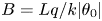 $B = Lq/k|\theta _0|$ given by (4.10a,b). For this, we begin by estimating the minimum thermal flux of a body of height
  $H$ using the scaling
  $q = D H^{-1/4}$ implied by (2.9), where
 \begin{equation} D \equiv \gamma {\rm \Delta} T_{air} k_{air} \left(\frac{{\rm \Delta} \rho_{air} g}{ \kappa_{air} \mu_{air}}\right)^{1/4}. \end{equation}
Here,  $k_{air} = 25 \times 10^{-3}$ W m
 $^{-1}$ K
 $^{-1}$ is the thermal conductivity of the air,
  $g = 9.81$ m s
 $^{-2}$,
  $\kappa _{air} = 2.0 \times 10^{-5}$ m
 $^2$ s
 $^{-1}$ is the thermal diffusivity of the air,
  $\mu _{air} = 18 \times 10^{-6}$ Pa s is the viscosity of the air and
  $\gamma \approx 0.50$ is the dimensionless coefficient determined from the solution of the boundary-layer system applicable for uniform fluid viscosity and diffusivity (Schlichting & Gersten Reference Schlichting and Gersten2017). Assuming that the ambient air is at a room temperature of
  $20\,^\circ$C far from the body (making
  ${\rm \Delta} T_{air} = 20$ K), the maximum density difference is
  ${\rm \Delta} \rho \approx 0.084$ kg m
 $^{-3}$. Using the above, we estimate
  $D \approx 55$ W m
 $^{-7/4}$. Assuming a cube with height
  $H = 2L$ and an initial temperature of
  $-10\,^\circ$C, we estimate the Biot number to be
  $B \approx 0.040$,
  $1.3$ and
  $40$ for sides of length
  $H = 1$ cm,
  $1$ m and
  $100$ m, respectively.
C.2. Travelling wave solution for the thermally thin limit
If the conduction within the body forms a thin boundary layer under the surface of the body then the finitude of the body has no effect on the evolution of the temperature, which approaches a steady state in a frame moving with the melting surface. In this regime, the solution is described to leading order by an exact travelling wave solution applicable for melting infinite slabs (e.g. Jaeger & Carslaw Reference Jaeger and Carslaw1959). By considering the steady solution to (4.8a–c) in the moving frame  $(\xi ,t)$, where
  $\xi =x - Ut$, and integrating the resulting equation subject to the surface condition
  $\theta = 0$ at
  $\xi = 0$ and the far-field condition
  $\theta \to -1$ as
  $\xi \to -\infty$, we obtain the solution as
 \begin{equation} \theta ={-}1 + \textrm{e}^{\varLambda[x - x_N(t)]}, \end{equation}
where  $\varLambda \equiv SB/(1+S)$ is the dimensionless recession speed. Recasting the recession speed in dimensional variables,
  $V = (\kappa /L)\varLambda$, we obtain (4.11). In this regime, melting and warming of the body occur in parallel, producing a linear proportionality between
  $V$ and the surface flux
  $q$. The interior of the body remains predominantly at the initial temperature during the evolution, as illustrated by case B of figure 9. This contrasts with case C, which involves two steps: an initial step of near uniform warming of the body to the melt temperature, followed by a second step in which the melting takes place (sensible and latent heating occur in series, rather than parallel). Since
  $\varLambda ^{-1}$ characterises the extent of the conductive layer in (C2), the regime represented by (C2) is self-consistent only if the extent of the layer is much less than that of the body,
  $\varLambda \gg 1$.
C.3. Total melt time
The total melt time for the Stefan problem given by (4.6a–c) and (4.7a,b) is given by a simple analytical expression representing the time necessary for the heat flux prescribed at the surface to supply all the sensible and latent heat needed both to warm and melt the solid. To derive this, we apply a definite spatial integral of (4.6a) over the extent of the solid, use Leibniz's theorem and impose (4.7a,b) to obtain
 \begin{equation} \frac{\textrm{d} }{\textrm{d} t} \int_0^{x_N(t)} \theta(x,t) \, \textrm{d} x = \theta_* \dot{x}_N + q. \end{equation}
Integration subject to the initial conditions (4.6a,b) gives
 \begin{equation} \int_0^{x_N(t)} \theta(x,t) \, \textrm{d} x = \theta_0 L - ( \theta_*[L - x_N(t)] + qt ), \end{equation}
which provides the total thermal energy in the system as a function of time. Setting  $x_N = 0$, we determine the total melt time to be
  $(|\theta _0| + \theta _{*})L/q$, representing the time needed to supply all the sensible and latent heat to melt the body fully. In dimensionless form, the time is
  $\tau = (1+S)/SB$, which we used in our computation of the ratio of the time to start melting to the total melt time used to produce figure 9.


 Open access