Article

Water Budgets of Managed Forests in Northeast Germany under Climate Change—Results from a Model Study on Forest Monitoring Sites

1
Faculty of Forest and Environment, University of Applied Science Eberswalde, Alfred-Möller-Str. 1, 16225 Eberswalde, Germany
2
Landeskompetenzzentrum Forst Eberswalde, Alfred-Möller-Str. 1, 16225 Eberswalde, Germany
3
Landesforst Mecklenburg-Vorpommern, Fritz-Reuter-Platz 9, 17139 Malchin, Germany
*
Author to whom correspondence should be addressed.
Appl. Sci. 2021, 11(5), 2403; https://doi.org/10.3390/app11052403
Submission received: 18 December 2020 / Revised: 2 March 2021 / Accepted: 3 March 2021 / Published: 8 March 2021
(This article belongs to the Special Issue Forest Soil Monitoring)

Abstract

:
To develop measures to reduce the vulnerability of forests to drought, it is necessary to estimate specific water balances in sites and to estimate their development with climate change scenarios. We quantified the water balance of seven forest monitoring sites in northeast Germany for the historical time period 1961–2019, and for climate change projections for the time period 2010–2100. We used the LWF-BROOK90 hydrological model forced with historical data, and bias-adjusted data from two models of the fifth phase of the Coupled Model Intercomparison Project (CMIP5) downscaled with regional climate models under the representative concentration pathways (RCPs) 2.6 and 8.5. Site-specific monitoring data were used to give a realistic model input and to calibrate and validate the model. The results revealed significant trends (evapotranspiration, dry days (actual/potential transpiration < 0.7)) toward drier conditions within the historical time period and demonstrate the extreme conditions of 2018 and 2019. Under RCP8.5, both models simulate an increase in evapotranspiration and dry days. The response of precipitation to climate change is ambiguous, with increasing precipitation with one model. Under RCP2.6, both models do not reveal an increase in drought in 2071–2100 compared to 1990–2019. The current temperature increase fits RCP8.5 simulations, suggesting that this scenario is more realistic than RCP2.6.

1. Introduction

Forests are of major importance in biogeochemical cycles and interact with climate [1]. Central European forests are endangered by drought events [2], which was particularly shown after the drought years in 2018 and 2019. Northeastern Germany is considered to belong to the regions that are most vulnerable to climate change-induced drought in Germany [3]. On a global scale, drought impacts on ecosystems have increased over the 20th century [4]. An increase in meteorological drought in spring and early summer could be shown for central Europe [5]. Case studies in northeast Germany revealed decreasing lake-levels of groundwater-fed lakes [6] and simulated decreasing groundwater recharge under a forested area [7] and an increasing number of drought days in forests [8]. The decline of water availability is the consequence of increasing temperature, which affects the frequency and intensity of drought periods with changes in evaporation and precipitation. For Germany, meteorological time series proved a temperature increase of 1.2 °C between 1881 and 2012 [9]. Apart from a direct effect on evaporative demand of the atmosphere, increasing temperature led to an earlier beginning of the vegetation period in the Northern Hemisphere, and thus to the increasing water use of the vegetation, which amplified soil drought in summer [10]. Furthermore, climate warming effects on atmospheric circulation significantly affect regional precipitation [11].
There is evidence that climate change increases drought impacts on tree growth and vitality, e.g., [12,13,14], and concomitant damages, such as insect attacks [15,16] or wildfires [17]. Due to climate change, forest planners are challenged by a precarious future. To develop measures to reduce the vulnerability of forests to drought, it is necessary to assess risk for tree species on site level [18,19]. Site-specific water balance modeling under the current climate and their development with climate change scenarios can support risk assessment.
To estimate the water balance of forests over long time-periods, site-specific data are necessary, which can be used to calibrate and validate water balance models, and which is detailed enough to differentiate between site conditions. In Germany and other European countries, monitoring data are available from the International Co-operative Program on Assessment and Monitoring of Air Pollution Effects on Forests (ICP Forests, www.icp-forests.net, [20]). Within the ICP-Forests Level II, monitoring network on comprehensively instrumented plots in selected forest ecosystems across Europe long-term permanent monitoring is conducted.
For Europe, regional climate projections are available from the Euro–Cordex initiative [21], which downscaled the global climate projections from the fifth phase of the Coupled Model Intercomparison Project (CMIP5). CMIP5 uses greenhouse gas concentration trajectories provided by the representative concentration pathway (RCP) scenarios. In RCP2.6, radiative forcing peaks at approximately 3 Wm−2 before 2100 and then declines; in RCP4.5 and RCP6.0, radiative forcing is stabilized at approximately 4.5 Wm−2 and 6.0 Wm−2, and in RCP8.5, radiative forcing reaches greater than 8.5 Wm−2 by 2100 and continues to rise [22]. CMIP5 based climate change studies come for different indicators to the result that southern Europe will become drier with a scenario (RCP)—dependent intensity, while in northern Europe, moisture will change less or increase [21,22,23,24,25]. For the region of northeast Germany, distinct drought indicators as a whole show no clear trend. Precipitation and the frequency of heavy rain events increase in central Europe under RCP4.5 and under RCP8.5 [21]. Soil moisture data of 26 general circulation models indicate a decrease in soil moisture when comparing the period 1971–2000 with 2071–2100 under RCP8.5 [24]. However, the results were robust only for soil moisture in autumn. The decrease of soil moisture was related to an increase in evapotranspiration, which exceeded changes in precipitation. The results of hydrological modeling based on data from five general circulation models indicate an increase in soil moisture drought events by 11% under the RCP2.6 and 19% under RCP6.0 [25]. The analysis of low flows in European rivers with distinct hydrological models and CMIP5 forcing yielded no clear change signal for northeast Germany under different warming levels [26]. A case study in the southwestern located region “Thüringer Becken” simulated an increasing, but non-robust, the tendency of groundwater levels and -recharges [27]. Because the resolution of European wide studies is too coarse to extract detailed information for forests in northeast Germany, a fine-scale study in that region is needed, that accounts for site-specific conditions.
The aim of our study is (a) to evaluate and to optimize the performance of the LWF-BROOK90 hydrological model (LWF, Freising, Germany) with measured soil moisture data, (b) to evaluate the changes in water budgets within the time period 1961–2019, and (c) to assess the future changes in water budgets under RCP2.6 and RCP8.5 with two regionalized CMIP5 models.

2. Materials and Methods

Our study used data from seven monitoring sites in northeast Germany (Figure 1). The sites are situated in the German states Berlin, Brandenburg, and Mecklenburg-Pomerania. Northeast Germany is located in a transition zone between oceanic and continental temperate climates. The coastal parts are directly influenced by the Baltic sea. Within the region, there is a climatic gradient from northwest to southeast toward an increasing continentality. The annual average temperature varies regionally between 8–9 °C. The average annual climatic water balance ranges from minimum values of about –200 mm in central Brandenburg to maximum values of about +200 mm in the north of Mecklenburg-Vorpommern. The parent materials are quaternary sediments. According to the results of the National Forest Soil Inventory for the topsoil, mainly glacial cover sands (60% of soils), glacial fluvial sand (17%), aeolian dune sand (10%), and glacial loam (5% in 10 cm depth; 10% in 100 cm depth) occur in forest soils [28]. Glacial marl appears in the subsoil of less than 5% of the forest soil. The study sites are mainly stocked with Scots pine ( five sites, Table 1) with a comparable age structure [29]. One site is a mixed Scots pine, pedunculate oak site, and one site is a European beech site. Sites 1203 and 1303 exhibit dense ground vegetation. Most of the soils are characterized as Brunic Arenosols by nutrient-poor sandy substrates. On sites 1203 and 1303, podzolization has advanced. Site 1202 contrasts to the other sites as Lamellic Arenosol with a higher water holding capacity due to the occurrence of bands of loamy sands in the subsoil. Moreover, sites 1203 and 1302 exhibit relatively higher water holding capacities. The substrate in 1203 is fine sand, and site 1302 is characterized by a low silt and clay content.
Since 1996, the seven monitoring sites are part of the ICP Forests Level II monitoring program, with the consequence that measurements on the sites are conducted according to a common protocol. The sites are equipped with a meteorological station and soil moisture content is measured in several soil layers by time domain reflectometry (TDR) sensors [30]. Forest mensuration data are collected [31], ground vegetation is surveyed by vegetation relevés [32], and soils are examined [33]. Soil analyses include measurements of carbon concentration, gravel content, bulk density, and particle size distribution. Within the last 10 years, also on-site measurements of leaf area index (LAI) started on all sites [34].
For water budget modeling, we used the LWF-BROOK90 hydrological model [35], which is a modification of the BROOK90 model [36]. BROOK90 is a process-based hydrologic model that simulates at point-scale vertical soil water movement and evapotranspiration at a daily time-step throughout the year. The model includes macropore-assisted infiltration, streamflow, and groundwater flow, in addition to modules to handle snow. Evaporation is calculated by the Shuttleworth–Wallace approach, which is a modification of the Penman–Monteith method to differentiate between soil evaporation and canopy transpiration [37]. It was designed to be applicable to canopies of any leaf area index (LAI) and developed further by Federer et al. [38] to be applicable for any land surface. The model estimates interception and transpiration from a single-layer plant canopy. Interception rates are assumed as a constant fraction of rainfall or snowfall per unit LAI and stem area index (SAI) for both forest canopy and ground vegetation. Partial canopy wetting and drying [39] are not considered. Transpiration is related to radiation, air temperature, and vapor pressure deficit due to stomatal control, according to [40]. The aerodynamic resistance for water vapor fluxes is obtained using daily mean wind speed and an approximated vertical wind profile. Soil water limitation of transpiration is calculated recognizing root density profiles, plant resistance, and a critical leaf water potential. Soil matric flow is modeled by the Richards equation. Hydraulic properties are derived according to Clapp and Hornberger [41] in BROOK90, while in LWF-BROOK90, a Mualem–van Genuchten parameterization [42] is also possible. The model operates with input about climate (temperature (min. and max.), precipitation, relative humidity, solar radiation, wind speed,) in daily time steps, leaf phenology, leaf area index, stem area index, stand height, fine root distribution, and soil hydraulic parameters.
To obtain complete daily climate time series from 1961 to 2019 for model input, we used in the first step the Deutscher Wetterdienst (DWD) station data [43] and interpolated it to the plots by means of ordinary kriging (precipitation) or regression kriging (all other meteorological variables) as described by Ziche et al. [44]. Then, in the second step, the measured time series from 1996 to 2019 were homogenized and gap filled with the interpolated time series [44]. In a final step, the interpolated time series was adjusted to the homogenized time series with means of quantile mapping [45], and both time series were merged.
Climate scenario data from the Euro–Cordex project with a spatial resolution of 0.11° and a daily time resolution from 2010 to 2100 was used [21]. These data are based on CMIP5-climate scenarios, which were downscaled by regional climate models. We worked with two combinations of global and regional circulation models, MPI-ESM-REMO (MPI/REMO) and EC-Earth-RCA4 (ECE/RCA4), and two RCPs (2.6, 8.5). The model behavior was already examined for Germany and revealed a larger temperature increase for ECE/RCA4 compared to MPI/REMO under both RCPs, while the latter shows an increase of precipitation, which is more pronounced under the RCP8.5 [46]. The climate scenario time series were bias-adjusted to the historical time series by means of quantile mapping [45].
Leaf Phenology was estimated by the model of Menzel and Fabian [47] and Hammel and Kennel [35], whose parameterization was optimized for northeast Germany. Stand height was calculated as the top height from measured tree heights. To estimate the tree height development from 1961 to 2019, the height development from digital yield tables [48] was adjusted to the measured heights. Leaf area index (LAI) was modeled by using the tree data of consecutive forest inventories in combination with allometric functions for individual tree biomass (see Ziche et al. [49] for more details), and specific leaf area (SLA) values from the database of life-history traits of Northwest European flora (LEDA) [50]. The stem area index (SAI) was estimated with diameter at breast height (DBH) based functions [51]. The development of LAI and SAI from 1961 to 2019 was estimated by applying the same functions to the yield tables, and by adjusting that LAI and SAI time series to the values estimated with the forest inventory data. The LAI of ground vegetation was estimated by determining the leaf biomass with vegetation surveys in combination with the Phytocalc model [52,53] and plant allometry [54]. Then the leaf biomass was multiplied with SLA values from the LEDA database [50]. Root distribution was estimated by modeling the fine root density according to a statistical model based on physical soil properties, soil organic matter, depths, and slope [55] and then fitting the depths distribution with the beta-model [56,57].
In LWF-BROOK90, the soil hydraulic parameterization depends on Mualem–van Genuchten parameters. These were derived from measured water retention curves for distinct soil horizons. Moreover, measured gravel content was available for the complete soil profiles down to a varying depth depending on the monitoring site. The data for deeper soil layers down to a depth of 4 m were derived either, if soil texture was available, by soil texture-based Mualem–van Genuchten values [58], or by assigning the values of the deepest soil layer that contains data. The tortuosity parameter l was set to 0.5.
We used default parameter values to run LWF-BROOK90 using the R–interface brook90r [59]. Exceptions were canopy and leaf parameters for which we used tree-specific values (stomatal conductance [60], winter LAI fraction [35], albedo, and leaf size [55], Table S1). We considered the canopies to be closed. Soil water flows were set to free drainage, no bypass-flow, and constant source area flow parameters and infiltration depth between all sites. We simulated soil hydrology of the organic layer and the mineral soil down to a depth of 4 m. The soil column was intersected in thinner layers starting with 1 cm in the organic layer and topsoil to increasing thickness up to 20 cm in the bottom layers.
The macropore infiltration parameter infexp was calibrated for each site. Therefore, infexp was varied stepwise between 0.01 and 1. Then the model output was compared with measurements. We used measurements of volumetric soil water content.
The historical time series 1961–2019 was modeled twice—one time with stand development as described above, and the second time with constant LAI, SAI, and height, which were derived from the year 2019. The future climate scenarios also run with these stand data. The first run was used for validating model performance with soil water content and interception values. The second run was used to examine the impact of climate change on water budgets. We used constant stand parameters to estimate the change between the historical time period and the scenarios without interactions to stand development.
In addition to LWF-Brook90, according to Food and Agriculture Organisation of the United Nations (FAO) we calculated grass reference evapotranspiration (PET [61]) and climate water balance (CWB).
From the variables obtained from the model output, we further calculated indicators for soil water supply and drought stress. We calculated plant-available soil water down to a depth of 200 cm (SW200) as
S W 200 = i = 1 n ( m i n θ i , θ f c i θ w p i ) × 1 c i × d i ,
where θ i = volumetric water content, θ f c i ,   θ w p i = volumetric water contents at field capacity (−6.3 kPa) and wilting point (−1583 kPa), c i = coarse fragment content, d i = layer thickness, and n = lowest layer in 200 cm depths, for layer i = 1 to layer n.
To indicate soil-moisture and drought-stress for the forests, we used the transpiration index, which is the ratio of actual to potential transpiration [62] and ranges between 0 and 1. We followed Schwärzel et al. [63] and defined days with a transpiration index below 0.7 as dry days (TI).
Our statistical evaluation is based on annual values. To evaluate the changes in water budgets within the time period 1961–2019 and to assess the future changes in water budgets, we used two approaches. First, the period 1961–1990 was compared with 1991–2019, and the latter was compared with 2071–2100 by means of ANOVA and t-test. Secondly, we assessed if a trend was significant within the historical time period from 1961 to 2019 and within the individual scenarios from 2010 to 2100. To test if trends within the historical time period or the scenarios were significant and differ between scenarios, a generalized mixed model, with scenario and time as fixed effects, was fitted as a random intercepts model with an unstructured correlation matrix (PROC GLIMMIX, SAS 9.4, SAS Institute Inc., Cary, NC, USA). For the water budget components precipitation, evapotranspiration, transpiration, SW200, and temperature, we fitted a lognormal distribution. For the variable dry days per year, we fitted a Poisson distribution, modified according to Joe and Zhu [64], to account for overdispersion. For climate water balance and seepage, a gaussian distribution was fitted. Inferences on differences of slopes between scenarios were made by specifying contrasts. Additionally, simple linear fixed-effects models with time as fixed effect were fitted for single plots. All statistics were fitted on a 95% confidence level. Statements about significance are made on p < 0.05 probability value. Test statistics can be found in Tables S2–S5 in the Supplementary Materials Section.

3. Results

3.1. Fitting Infiltration Parameter Infexp

To select the best fitting infexp value, the results of all depths equipped with sensors were evaluated. Figure 2 shows for four depths per site the r2 of the correlation between measured and modeled soil water content for various infexp values. The results indicate by variations between infexp values, that the influence of infexp varied between the sites— in site 1202, it was highest. The r2 exhibited a high variation between infexp values at the lowest measurement depths (Figure 2, right column), In contrast, in site 1302, infexp had nearly no influence. There, the r2 varied less between infexp values.
After optimizing the infiltration parameter infexp, we assigned the following infexp values to the sites 1101: 0.4; 1202: 0.8; 1203: 0.6; 1204: 0.8; 1205: 0.2; 1302: 0.2; and 1303: 1.0. The lower the infexp value is, the more water is fed to the upper soil layers, while an infexp value of 1.0 distributes the water evenly within the soil column up to maximum infiltration depths.

3.2. Model Validation

For soil moisture content (theta) the comparison between measurements and model outcome yielded r2 values between 0.4 and 0.9 (Figure 2). The average r² for each site were 0.82 in 1101, 0.60 in 1202, 0.75 in 1203, 0.77 in 1204, 0.82 in 1205, 0.69 in 1302, and 0.66 in 1303.
To evaluate interception, we compared the measured net rainfall (rainfall below tree canopy) with its modeled counterpart (rainfall reaching the ground). On all sites measured net rainfall was larger than modeled values. The difference between measured and modeled net rainfall amounted to 0% to 9% from open field rainfall. For temperatures ≥4 °C the r2 of the regression were high, 0.88–0.95. For temperature ≤4 °C the r2 of the regression was 0.80–0.88 lower than for temperatures ≥4 °C.

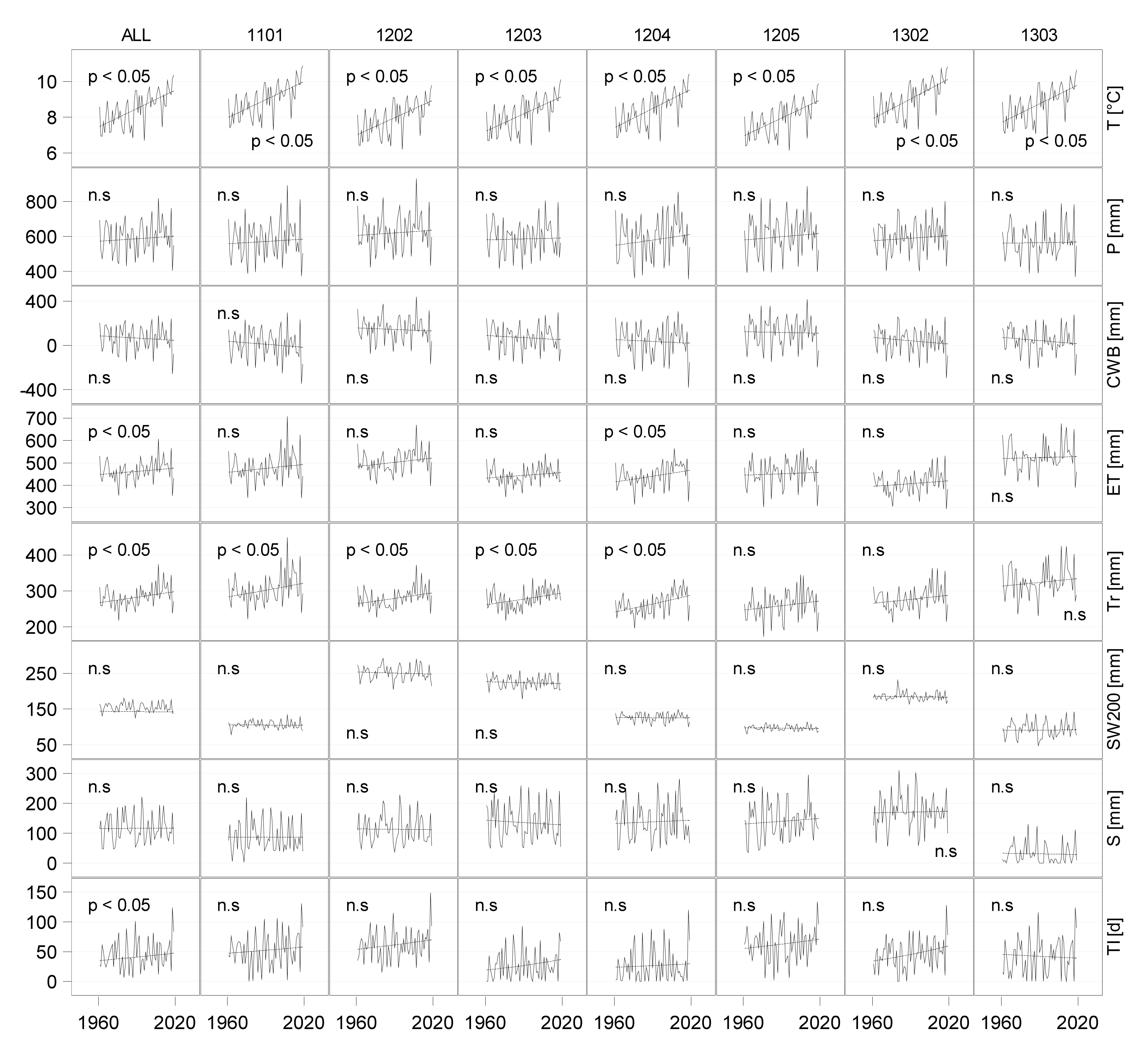
3.3. Water Budgets of Historical Time Series

When comparing the period 1961–1990 with 1991–2019, the temperature increased by ~1 °C from 8.0 ± 0.2 °C to 9.0 ± 0.2 °C (Table 2, Table S2). This increase was constant over all sites (Figure 3). Within the whole time period 1961–2019, a linear trend was significant (Figure 3, Table S3). With 9.5 ± 0.3 °C, the current decade is 0.6 °C warmer compared to the preceding decade.
With 584 ± 16 mm to 609 ± 18 mm, precipitation did not increase significantly (Table 2). The decade 2001–2010 had the highest precipitation values with 644 ± 33 mm on average. Precipitation in the current decade is 592 ± 38 mm lower. In none of the sites, a significant linear trend was evident (Figure 3).
The temperature increase was accompanied by a significant increase of PET from 513 ± 6 mm to 548 ± 7 mm on average between both time periods. The increase was significant on all sites. CWB did not change significantly.
Actual evaporation increased significantly from 454 ± 7 mm in 1961–1990 to 480 ± 9 mm in 1991–2019. Moreover, transpiration increased from 274 ± 4 mm to 296 ± 6 mm. A linear trend was significant for transpiration and actual evapotranspiration within the whole period 1961–2019 (Figure 3). Seepage and soil water storage down to 2 m (SW200) remained unchanged between both periods.
The number of dry days per year (TI) did not increase significantly between the periods 1961–1990 and 1991–2019 with 42 ± 4 days to 49 ± 5 days (Table 2), but a linear trend was significant over the whole period (Figure 3, Table S3). The change between both periods was significant on the beech site 1302, where it increased from 40 ± 4 days to 52 ± 5 days. The current decade exhibited, with 56 ± 11 days on average, the highest number of dry days.
Our results demonstrate that 2018 was the driest year on average within the historical time period 1961–2019. This is shown by precipitation with 404 ± 15 mm, climatic water balance with −259 ± 30 mm, transpiration with 237 ± 12 mm, and 124 ± 7 dry days (Figure 3). Soil water content is in 2018 with 139 ± 20 mm not as extreme as the other indicators, and with 177 ± 19 mm, seepage is even higher than the average (Table 2), but in 2019 seepage is, with 74 ± 12 mm, distinctly lower and soil water content keeps, with 137 ± 19 mm, the same level compared to 2018. That the year 2019 was also a dry year is further indicated by precipitation with 550 ± 11 mm, climatic water balance with −79 ± 23 mm, transpiration with 272 ± 6 mm, and with 83 ± 4 dry days.

3.4. Water Budgets under Future Climate

The temperature (T) increased under RCP2.6 with MPI/Remo and ECE/RCA4 comparing 2071–2100 with the 1991–2018 time period by 0.6 °C and 0.7 °C, respectively (Table 2, Table S2). Under the RCP8.5, the temperature increased by 2.6 °C and 3.6 °C between both time periods, respective. A linear trend was significant within all simulations (Figure 4, Table S3). The slopes of MPI/Remo RCP8.5 and the historical time period did not differ significantly (Figure 4). ECE/RCA4 under RCP8.5 showed the steepest temperature increase (Table S4).
Precipitation (P) did not change significantly under the RCP2.6. In the time period 1991–2019, it amounted to 609 ± 18 mm on average, and in 2071–2100, to 638 ± 17 mm with MPI/Remo, and to 629 ± 17 mm with ECE/RCA4. Under the RCP8.5, precipitation increased significantly to 716 ± 15 mm with MPI/Remo, while the change to 654 ± 19 mm with ECE/RCA4 was not significant. Within the scenarios, also a linear trend was significant under RCP8.5 with MPI/Remo (Figure 4).
Potential evapotranspiration (PET) increased under RCP2.6 from 548 ± 7 mm to 643 ± 8 mm with MPI/Remo and to 642 ± 10 mm with ECE/RCA4. Under RCP8.5, PET increased to 655 ± 10 mm with MPI/Remo and to 718 ± 12 mm with ECE/RCA4. An increasing linear trend was significant for all simulations, with exception of ECE/RCA4 RCP2.6. The slopes of ECE/RCA4 RCP8.5 and the historical time period did not differ significantly.
Climate water balance (CWB) decreased significantly with ECE/RCA4 RCP8.5 from 61 ± 22 mm to −64 ± 27 mm. With MPI/Remo RCP8.5 and with both models under RCP2.6, the changes to 1991–2019 were not significant. With ECE/RCA4 under RCP8.5, a linear decrease of CWB was significant.
Total actual evapotranspiration (ET) did not change on average with any of the climate change scenarios in comparison with 1990–2019, but a linear trend was significant within MPI/Remo under RCP8.5 and with ECE/RCA4 under both scenarios (Figure 4).
Seepage (S) increased significantly under RCP8.5 with MPI/Remo in 2071–2100 compared to 1991–2019 from 116 ± 8 mm to 208 ± 13 mm. Under RCP2.6, the increase was not significant. With ECE/RCA4, seepage did not change significantly under both scenarios in comparison with 1991–2019. Within the scenarios, trends were significant with both models under RCP8.5—seepage increased significantly within MPI/Remo and decreased within ECE/RCA4. Within RCP2.6, seepage also declined significantly with ECE/RCA4.
Soil water storage, down to 2 m (SW200), did not change under RCP2.6 and under RCP8.5 in 2071–2100 in comparison with 1991–2019, but within ECE/RCA4 under RCP8.5, a decreasing trend was significant (Figure 4).
The number of dry days (TI) per year did not change significantly under RCP2.6 between the periods 1991–2019 and 2071–2100. Under RCP8.5, ECE/RCA4 revealed a significant increase to 51 ± 3 days, while with MPI/Remo, the number of dry days was, with 25 ± 3 in 2071–2100, lower than 1991–2019. However, under RCP8.5 with both models, dry days increased significantly within 2010–2100. In comparison to the trendline of the historical time period, an offset was apparent (Figure 4).

4. Discussion

The sites of ICP Forest Level II enabled hydrological modeling with realistic site-based input data and model validation. In the model validation section, we show that our model setup reproduces measurements, expressed by interception and soil water content.
Modeled interception was higher than measured, probably due to the lacking measurements of interception by the ground vegetation. Unfortunately, most research studies focus on forest canopy interception and why direct measurements of ground vegetation interception are rare [65]. Based on the modeled daily net rainfall and the measured throughfall in the rain gauge, the amount of the ground vegetation interception of the four pine stands examined ranged between 0% and 9% of annual gross rainfall. However, partitioning of gross rainfall into interception, throughfall, and stemflow is strongly influenced by stand characteristics and might vary between seasons and years due to different rainfall conditions [66]. Thus, the role of ground vegetation interception cannot be described precisely. Nevertheless, we consider a reliable estimate of daily throughfall rates as soil water predictions have been in good agreement with measurements.
The simulation results indicate that tuning the infiltration parameter infexp could improve on some sites the soil water predictions, while at others, it had less influence. In BROOK90, macropore-assisted infiltration is not explicitly modeled. Nevertheless, incoming water can be partitioned across the soil column by the infiltration parameters, and thus, preferential flows are represented.
Preferential flows exhibit a high small-scale spatial variability and are influenced by stemflow and rooting, e.g., [67,68]. Water is collected by tree crowns and conducted via stem and roots to the soil causing a greater infiltration depth nearby the trunks [69]. This effect is influenced by species [70]. Beech trees have a larger partitioning of gross precipitation to stemflow compared to pine trees and might have a substantial effect on the groundwater recharge in the direct surrounding of beech trees [71].
Because the soil moisture measurements on the ICP Forests Level II sites are undertaken with three replications, these measurements do not account for small-scale variance. Furthermore, because the sondes are placed at a distance to the stems, the probability is higher that infiltrated water originates from throughfall than from stemflow. Therefore, model optimization also reflects the throughfall-descended rather than stemflow-descended infiltration. However, by varying infexp, we were able to fit the simulated infiltration distribution to the measured soil water contents in different depths at each site. The average r² ranged from 0.60 to 0.82 and confirmed reliable predictions of soil moisture at all sites.
The modeled actual transpiration is limited by the water supply rate controlled by the water potential gradient and plant resistance and is, thus, depending on reliable soil moisture predictions and maximum root water uptake, respectively. We obtained reliable stand transpiration rates compared to other studies. Based on sap flow measurements, pine canopy transpiration within the growing season ranged between 112 mm and 239 mm, depending on stand age, site condition, and year [72,73,74]. Because we cannot separate canopy and ground vegetation transpiration, a direct comparison to [72,73,74] is not possible. Nevertheless, based on results from Vincke and Thiry [74] and Müller [75], we conclude that the transpiration of ground vegetation is higher than 50% of pine canopy transpiration. Therefore, our results obtained for the five pine stands, 331 ± 19 mm in the moist year 2017, 242 ± 20 mm in the drought year 2018, and 294 ± 6 mm on average in the period 1991–2019, are in the range of [72,73,74] when recognizing ground vegetation. In the beech site, stand examined the transpiration of ground vegetation is neglectable so that a direct comparison with results obtained from sap flow measurements is possible. There, we obtained annual transpiration of 356 mm in the moist year 2017 and 214 mm in the very dry year 2018. The average for the period 1991–2019 amounted to 287 ± 7 mm. Again, based on sap flow measurements, beech canopy transpiration within the growing season ranged between 250 mm and 350 mm [76,77,78,79,80].
Our model approach revealed that the rise of temperature during the last decades is accompanied by an increase in transpiration. In fact, seasonal variations of the terrestrial evapotranspiration are positively correlated with temperature in Europe [81] and showed an increasing trend at a global scale within the last decades [82]. However, actual canopy transpiration is obviously limited by soil moisture and the hydraulic conductance from bulk soil to leaf [83]. In our simulations, we could show that the temperature increase comes along with drier conditions as shown by the increasing number of dry days per year indicated the transpiration index (Figure 4).
In particular, the last two drought years 2018 and 2019 pushed forest damages in the study region. With the year 2020, we now observed the third consecutive year of drought. As obtained by the large-scale forest condition monitoring of the ICP Forests network (Level I), defoliation and tree mortality has increased in almost all tree species in recent years [84,85]. In the study region, pines showed the highest defoliation since the beginning of the 1990s, accompanied by biotic damages, leading to the death of individual trees. Beech trees showed the highest records of defoliation in the year 2019, and especially old trees obtained dieback of the crown starting from the top.
Our study revealed that 2018 was the most severe drought year within the whole period 1961–2019. In 2019 seepage was distinctly lower than in 2018, while soil water content kept on a low level comparable with 2018. As shown by the climate water balance (Figure 3), the year 2018 ended up with the highest water deficit observed on all sites (with exception of site 1203) within the whole period. The lack of winter precipitation and consequential refilling of the soil water body most likely reinforced the impact of drought conditions in 2019, especially at the beginning of the growing season. Furthermore, the depletion of the internal water storage during subsequent drought years obviously affects the whole-tree water relationship [86]. For example, Betsch et al. [87] observed an increase in the contribution of whole-plant exchangeable water to daily transpiration of a young beech stand during the drought of 2003 (with a moist year in front) to 67% in maximum. Hysteresis effects are not considered in the model approach that applied to why actual transpiration might be even overestimated in periods of prolonged drought. The strong decrease of the modeled seepage water in 2019, furthermore, indicates the impact of the subsequent drought years and the decline in plant-available soil water. This effect, however, might be more important at sites of high water-holding capacity compared to sandy soils. Tor-Ngern et al. [88] showed that in pine stands canopy, transpiration was sensitive to decreasing soil moisture at an earlier point of relative extractable water in loamy than sandy soils. The increase of dry days (TI; Figure 3) of pine stands in the last two years accompanies the strong increase in defoliation of pine trees in the study region in 2019. Thus, we argue that pine stands are vulnerable to subsequent drought years due to the depletion of both soil and whole-tree water reservoirs, which might increase in the future (Figure 4).
It has been shown that water budget components of Scots pine forests could be influenced by forest management [7,75]. Tree species selection is an important management tool to mitigate the consequences of climate change [89]. Scots pine plantations in northeast Germany are subjected to forest conversion toward more diverse forests with higher broad leaf percentages [90]. This will help to increase seepage discharge and thus improve the hydrological status of the region. On the other hand, the vulnerability of the different tree species toward climate change must be considered [91]. Modeling stand water budgets are considered an important tool to reconsider species–specific thresholds in drought tolerance and future prospective, e.g., [92]. For the state of Brandenburg, a concept is developed, based on species–site relationships, which makes suggestions about tree selection under climate change scenarios [19].
In respect to the climate projections considered, we obtained a significant positive trend in actual evapotranspiration for three of the four cases. Despite bias adjustment by the means of quantile mapping, the results reveal a non-significant bias in dry days between historical time series and future climate scenarios. This indicates a higher drought toward the end of the historical time period than at the beginning of the climate change simulations. Indeed, during the last decade, a high number of record-breaking temperature anomalies could be observed globally [93] and regionally for northeast Germany [94]. The current temperature increase fits well with the projected temperature increase under RCP8.5. Therefore, this scenario seems to be more likely to realize than RCP2.6. Our study comes to the result that under RCP8.5 drought, in terms of dry days, it will increase with both models, while drought in terms of climatic water balance and soil moisture content will increase only with ECE/RCA4 under RCP8.5. MPI/Remo show increasing precipitation under RCP8.5, which partly compensates for increasing water losses due to evapotranspiration and leads to an increase of seepage. Due to the dependency of precipitation to atmospheric circulation and their changes, e.g., [11,95], uncertainty in the simulation of regional precipitation in climate change models is high, and the models show high variability in simulated precipitation, e.g., [46,96,97].
Furthermore, hydrological models do not account for the effects of rising CO2 concentrations on plants [25]. The gas exchange of CO2 and water are closely interrelated; therefore, water budgets of plants interact with rising CO2 concentrations [98]. Vegetation is expected to counteract increasing drought, e.g., by changes in allocation patterns. In consequence, this could lead to an overestimation of drought stress by hydrological models, which did not account for CO2. Therefore, we conclude that it is highly uncertain to which extent climate change will affect the water budgets of forests in northeast Germany. Forest planners must take account of the current trend toward drier climate and of uncertain future conditions. Moreover, the current trend of an increase in canopy mortality in Europe will cause demographic changes in European forests [99], thus altering the properties and water relation of the soil-plant-atmosphere continuum in forests.
Nevertheless, the predicted increase of actual evapotranspiration and number of dry days shown in this study and the widely observed tree damages as a result of the last two drought years (2018 to 2019) demonstrate a high vulnerability of the forest trees in northeast Germany. Forest water budget modeling should hence accompany the ongoing effort of the establishment of mixed stands for risk-sharing in climate change, revealing species-specific thresholds of drought tolerance. Both the susceptibility toward drought of mature forests stands and the understory need to be considered in forest management strategies mitigating the consequences of climate change.

5. Conclusions

To study the impact of drought on forests in northeast Germany by means of water budget modeling, a valid model setup is needed. This is crucial for extending site-specific water balance modeling to sites where no measurements are available and to different scenarios of stand development and stand composition. Therefore, our aim was to evaluate and optimize the performance of the hydrological model with measured soil moisture data. Our evaluation of the modeling approach yields a good correlation of modeled output with measurements. We conclude that our model setup provides the basis for studying forest water budgets under changing climate and management.
One of the aims of our study was to evaluate the changes in water budgets within the time period 1961–2019. We could show that within the historical time period, evapotranspiration increased in parallel to temperature, which leads due to unchanged precipitation to an increase of dry days. Especially, the last two years of the time series were extreme. We conclude, based on the observed trend in our study and on observations on forest damages made in this region, that forests in northeast Germany are exposed to increasing drought risk. Our assessment of the future changes in water budgets under RCP2.6 and RCP8.5 with two regionalized CMIP5 models concludes that under RCP8.5, drought conditions will increase, in contrast to RCP2.6. The increase of temperature, evapotranspiration, and dry days within the historical time series is more in line with RCP8.5 than RCP2.6, suggesting that this scenario is more likely than RCP2.6. Changes in amounts of precipitation differ between both models within RCP8.5, indicating a high uncertainty in simulations of precipitation. In consequence, forest planners are faced with an uncertain future with respect to the water supply of forests. To minimize the risk, forest planning should focus on these uncertainties, e.g., by relying on diverse, species-rich forests.

Supplementary Materials

The following are available online at https://www.mdpi.com/2076-3417/11/5/2403/s1, Table S1: Ranges of parameter values, Table S2: Two-sided hypothesis-test statistics for pairwise comparison of periods 1961–1990, 1991–2019, and 2071–2100, Table S3: Two-sided hypothesis-test statistics for the significance of slope within the scenarios, Table S4: Two-sided test statistics for pairwise comparison for the difference of slopes, Table S5: Two-sided hypothesis-test statistics for the significance of intercept of random effect (site) within the historical time series.

Author Contributions

Conceptualization, D.Z. and W.R.; methodology, D.Z., A.R., and R.H.; software, D.Z.; validation, D.Z.; formal analysis, D.Z.; investigation, D.Z.; resources, W.R.; data curation, A.R., R.H., and J.M.; writing—original draft preparation, D.Z.; writing—review and editing, D.Z., W.R., R.H., A.R., and J.M.; visualization, D.Z.; supervision, W.R.; project administration, W.R.; funding acquisition, W.R. and J.M. All authors have read and agreed to the published version of the manuscript.

Funding

This research received no external funding.

Institutional Review Board Statement

Not applicable.

Informed Consent Statement

Not applicable.

Data Availability Statement

The data presented in this study are available on request from the corresponding author.

Acknowledgments

We thank all colleagues who were involved in field sampling and laboratory measurements. We thank the Bayrische Landesanstalt für Wald und Forstwirtschaft (LWF Freising) for providing the hydrological model LWF-BROOK90.

Conflicts of Interest

The authors declare no conflict of interest.

References

  1. Bonan, G.B. Forests and climate change: Forcings, feedbacks, and the climate benefits of forests. Science 2008, 320, 1444–1449. [Google Scholar] [CrossRef] [Green Version]
  2. Adams, H.D.; Zeppel, M.J.B.; Anderegg, W.R.L.; Hartmann, H.; Landhäusser, S.M.; Tissue, D.T.; Huxman, T.E.; Hudson, P.J.; Franz, T.E.; Allen, C.D.; et al. A multi-species synthesis of physiological mechanisms in drought-induced tree mortality. Nat. Ecol. Evol. 2017, 1, 1285–1291. [Google Scholar] [CrossRef] [PubMed]
  3. Lasch-Born, P.; Suckow, F.; Gutsch, M.; Reyer, C.; Hauf, Y.; Murawski, A.; Pilz, T. Forests under climate change: Potential risks and opportunities. Meteorol. Z. 2015, 24, 157–172. [Google Scholar] [CrossRef]
  4. Schwalm, C.W.; Anderegg, W.R.L.; Michalak, A.M.; Fisher, J.B.; Biondi, F.; Koch, G.; Litvak, M.; Ogle, K.; Shaw, J.D.; Wolf, A.; et al. Global patterns of drought recovery. Nature 2017, 548, 202–205. [Google Scholar] [CrossRef] [PubMed]
  5. Hänsel, S.; Ustrnul, Z.; Łupikasza, E.; Skalak, P. Assessing seasonal drought variations and trends over Central Europe. Adv. Water Resour. 2019, 127, 53–75. [Google Scholar] [CrossRef]
  6. Kaiser, K.; Koch, P.J.; Mauersberger, R.; Stüve, P.; Dreibrodt, J.; Bens, O. Detection and attribution of lake-level dynamics in north-eastern central Europe in recent decades. Reg. Environ. Chang. 2014, 14, 1587–1600. [Google Scholar] [CrossRef]
  7. Natkhin, M.; Steidl, J.; Dietrich, O.; Dannowski, R.; Lischeid, G. Differentiating between climate effects and forest growth dynamics effects on decreasing groundwater recharge in a lowland region in Northeast Germany. J. Hydrol. 2012, 448–449, 245–254. [Google Scholar] [CrossRef]
  8. Bauwe, A.; Criegee, C.; Glatzel, S.; Lennartz, B. Model-based analysis of the spatial variability and long-term trends of soil drought at Scots pine stands in northeastern Germany. Eur. J. For. Res. 2012, 131, 1013–1024. [Google Scholar] [CrossRef]
  9. Kaspar, F.; Müller-Westermeier, G.; Penda, E.; Mächel, H.; Zimmermann, K.; Kaiser-Weiss, A.; Deutschländer, T. Monitoring of climate change in Germany—Data, products and services of Germany’s National Climate Data Centre. Adv. Sci. Res. 2013, 10, 99–106. [Google Scholar] [CrossRef] [Green Version]
  10. Lian, X.; Piao, S.; Li, L.Z.X.; Li, Y.; Huntingford, C.; Ciais, P.; Cescatti, A.; Janssens, I.A.; Peñuelas, J.; Buermann, W.; et al. Summer soil drying exacerbated by earlier spring greening of northern vegetation. Sci. Adv. 2020, 6, 1. [Google Scholar] [CrossRef] [PubMed] [Green Version]
  11. Xie, S.; Deser, C.; Vecchi, G.A.; Collins, M.; Delworth, T.L.; Hall, A.; Hawkins, E.; Johnson, N.C.; Cassou, C.; Giannini, A.; et al. Towards predictive understanding of regional climate change. Nat. Clim. Chang. 2015, 5, 921–930. [Google Scholar] [CrossRef]
  12. Choat, B.; Jansen, S.; Brodribb, T.J.; Cochard, H.; Delzon, S.; Bhaskar, R.; Bucci, S.J.; Feild, T.S.; Gleason, S.M.; Hackel, U.G.; et al. Global convergence in the vulnerability of forests to drought. Nature 2012, 491, 752–756. [Google Scholar] [CrossRef] [Green Version]
  13. Yuan, W.; Zheng, Y.; Piao, S.; Ciais, P.; Lombardozzi, D.; Wang, Y.; Ryu, Y.; Chen, G.; Dong, W.; Hu, Z.; et al. Increased atmospheric vapor pressure deficit reduces global vegetation growth. Sci. Adv. 2020, 5, 8. [Google Scholar] [CrossRef] [Green Version]
  14. Bose, A.K.; Gessler, A.; Bolte, A.; Bottero, A.; Buras, A.; Cailleret, M.; Camarero, J.J.; Haeni, M.; Hereş, A.M.; Hevia, A.; et al. Growth and resilience responses of Scots pine to extreme droughts across Europe depend on predrought growth conditions. Glob. Change Biol. 2020, 26, 4521–4537. [Google Scholar] [CrossRef] [PubMed]
  15. Anderegg, W.R.L.; Hicke, J.A.; Fisher, R.A.; Allen, C.D.; Aukema, J.; Bentz, B.; Hood, S.; Lichstein, J.W.; Macalady, A.K.; McDowell, N.; et al. Tree mortality from drought, insects, and their interactions in a changing climate. New Phytol. 2015, 208, 674–683. [Google Scholar] [CrossRef]
  16. Netherer, S.; Panassiti, B.; Pennerstorfer, J.; Matthews, B. Acute Drought Is an Important Driver of Bark Beetle Infestation in Austrian Norway Spruce Stands. Front. For. Glob. Chang. 2019, 2, 39. [Google Scholar] [CrossRef] [Green Version]
  17. Jolly, W.M.; Cochrane, M.A.; Freeborn, P.H.; Holden, Z.A.; Brown, T.J.; Williamson, G.J.; Bowman, D.M.J.S. Climate-induced variations in global wildfire danger from 1979 to 2013. Nat. Commun. 2015, 6, 7537. [Google Scholar] [CrossRef] [PubMed]
  18. Riek, W.; Russ, A. In Zeiten des Standortswandels: Handlungsempfehlungen aus BZE und Regionalisierung für die nachhaltige Waldnutzung. In Eberswalder Forstliche Schriftenreihe, Bd. 67; Landesbetrieb Forst Brandenburg, Landeskompetenzzentrum Forst Eberswalde: Eberswalde, Germany, 2019; pp. 33–42. [Google Scholar]
  19. Riek, W.; Russ, A.; Grüll, M. Zur Abschätzung des standörtlichen Anbaurisikos von Baumarten im Klimawandel im nordostdeutschen Tiefland. In Eberswalder Forstliche Schriftenreihe, Bd. 69; Landesbetrieb Forst Brandenburg, Landeskompetenzzentrum Forst Eberswalde: Eberswalde, Germany, 2020; pp. 48–70. [Google Scholar]
  20. Fleck, S.; Cools, N.; De Vos, B.; Meesenburg, H.; Fischer, R. The Level II aggregated forest soil condition database links soil physicochemical and hydraulic properties with long-term observations of forest condition in Europe. Ann. For. Sci. 2016, 73, 945–957. [Google Scholar] [CrossRef] [Green Version]
  21. Jacob, D.; Petersen, J.; Eggert, B.; Alias, A.; Christensen, O.B.; Bouwer, L.M.; Braun, A.; Colette, A.; Déqué, M.; Georgievski, G.; et al. EURO-CORDEX: New high-resolution climate change projections for European impact research. Reg. Environ. Chang. 2014, 14, 563–578. [Google Scholar] [CrossRef]
  22. Moss, R.H.; Edmonds, J.A.; Hibbard, K.A.; Manning, M.R.; Rose, S.K.; van Vuuren, D.P.; Carter, T.R.; Emori, S.; Kainuma, M.; Kram, T.; et al. The Next Generation of Scenarios for Climate Change Research and Assessment. Nature 2010, 463, 747–756. [Google Scholar] [CrossRef]
  23. Samaniego, L.; Thober, S.; Kumar, R.; Wanders, N.; Rakovec, O.; Pan, M.; Zink, M.; Sheffield, J.; Wood, E.F.; Marx, A. Anthropogenic warming exacerbates European soil moisture droughts. Nat. Clim. Change 2018, 8, 421–426. [Google Scholar] [CrossRef]
  24. Ruosteenoja, K.; Markkanen, T.; Venäläinen, A.; Räisänen, P.; Peltola, H. Seasonal soil moisture and drought occurrence in Europe in CMIP5 projections for the 21st century. Clim. Dyn. 2018, 50, 1177–1192. [Google Scholar] [CrossRef] [Green Version]
  25. Grillakis, M.G. Increase in severe and extreme soil moisture droughts for Europe under climate change. Sci. Total Environ. 2019, 660, 1245–1255. [Google Scholar] [CrossRef]
  26. Marx, A.; Kumar, R.; Thober, S.; Rakovec, O.; Wanders, N.; Zink, M.; Wood, E.F.; Pan, M.; Sheffield, J.; Samaniego, L. Climate change alters low flows in Europe under global warming of 1.5, 2, and 3 °C. Hydrol. Earth Syst. Sci. 2018, 22, 1017–1032. [Google Scholar] [CrossRef] [Green Version]
  27. Jing, M.; Kumar, R.; Heße, F.; Thober, S.; Rakovec, O.; Samaniego, L.; Attinger, S. Assessing the response of groundwater quantity and travel time distribution to 1.5, 2, and 3 °C global warming in a mesoscale central German basin. Hydrol. Earth Syst. Sci. 2020, 24, 1511–1526. [Google Scholar] [CrossRef] [Green Version]
  28. Riek, W.; Russ, A.; Martin, J. Soil acidification and nutrient sustainability of forest ecosystems in the northeastern German lowlands—Results of the national forest soil inventory. Folia For. Pol. Series A 2012, 54, 187–195. [Google Scholar]
  29. Russ, A.; Riek, W.; Hentschel, R.; Hannemann, J.; Barth, R.; Becker, F. Wasserhaushalt im Trockenjahr 2018 —Ergebnisse aus dem Level II Programm in Brandenburg. In Eberswalder Forstliche Schriftenreihe, Bd. 67; Landesbetrieb Forst Brandenburg, Landeskompetenzzentrum Forst Eberswalde: Eberswalde, Germany, 2019; pp. 11–24. [Google Scholar]
  30. Raspe, S.; Beuker, E.; Preuhsler, T.; Bastrup-Birk, A. Part IX: Meteorological Measurements. In Manual on Methods and Criteria for Harmonized Sampling, Assessment, Monitoring and Analysis of the Effects of Air Pollution on Forests; UNECE ICP Forests Programme Co-ordinating Centre, Ed.; Thünen Institute of Forest Ecosystems: Eberswalde, Germany, 2016; p. 14. [Google Scholar]
  31. Dobbertin, M.; Neumann, M. Part V: Tree Growth. In Manual on Methods and Criteria for Harmonized Sampling, Assessment, Monitoring and Analysis of the Effects of Air Pollution on Forests; UNECE ICP Forests Programme Co-ordinating Centre, Ed.; Thünen Institute of Forest Ecosystems: Eberswalde, Germany, 2016; p. 17. [Google Scholar]
  32. Canullo, R.; Starlinger, F.; Granke, O.; Fischer, R.; Aamlid, D. Part VI.1: Assessment of Ground Vegetation. In Manual on Methods and Criteria for Harmonized Sampling, Assessment, Monitoring and Analysis of the Effects of Air Pollution on Forests; UNECE ICP Forests Programme Co-ordinating Centre, Ed.; Thünen Institute of Forest Ecosystems: Eberswalde, Germany, 2016; p. 12. [Google Scholar]
  33. Cools, N.; De Vos, B. Part X: Sampling and Analysis of Soil. In Manual on Methods and Criteria for Harmonized Sampling, Assessment, Monitoring and Analysis of the Effects of Air Pollution on Forests; UNECE ICP Forests Programme Co-ordinating Centre, Ed.; Thünen Institute of Forest Ecosystems: Eberswalde, Germany, 2016; p. 115. [Google Scholar]
  34. Fleck, S.; Raspe, S.; Cater, M.; Schleppi, P.; Ukonmaanaho, L.; Greve, M.; Hertel, C.; Weis, W.; Rumpf, S.; Thimonier, A.; et al. Part XVII: Leaf Area Measurements. In Manual on Methods and Criteria for Harmonized Sampling, Assessment, Monitoring and Analysis of the Effects of Air Pollution on Forests; UNECE ICP Forests Programme Co-ordinating Centre, Ed.; Thünen Institute of Forest Ecosystems: Eberswalde, Germany, 2016; p. 34. [Google Scholar]
  35. Hammel, K.; Kennel, M. Charakterisierung und Analyse der Wasserverfügbarkeit und des Wasserhaushalts von Waldstandorten in Bayern mit dem Simulationsmodell Brook90. In Forstliche Forschungsberichte München 185; Heinrich Frank: München, Germany, 2001; p. 135. [Google Scholar]
  36. Federer, C.A. BROOK 90: A Simulation Model for Evaporation, Soil Water, and Streamflow. 2002. Available online: http://www.ecoshift.net/brook/brook90.htm (accessed on 31 July 2020).
  37. Shuttleworth, W.J.; Wallace, J.S. Evaporation from sparse crops-an energy combination theory. Q. J. R. Meteorol. Soc. 1985, 111, 839–855. [Google Scholar] [CrossRef]
  38. Federer, C.A.; Vörösmarty, C.; Fekete, B. Intercomparison of methods for calculating potential evaporation in regional and global water balance models. Water Resour. Res. 1996, 32, 2315–2321. [Google Scholar] [CrossRef]
  39. Rutter, A.J.; Kershaw, K.A.; Robins, P.C.; Morton, A.J. A predictive Model of Rainfall Interception in Forests. Agric. Meteorol. 1972, 9, 367–384. [Google Scholar] [CrossRef]
  40. Jarvis, P.G. The interpretation of the variations in leaf water potential and stomatal conductance found in canopies in the field. Phil. Trans. R. Soc. Lond. B 1976, 273, 593–610. [Google Scholar] [CrossRef]
  41. Clapp, R.B.; Hornberger, G.M. Empirical equations for some soil hydraulic properties. Water Resour. Res. 1978, 14, 601–604. [Google Scholar] [CrossRef] [Green Version]
  42. Van Genuchten, M.T. A closed-form equation for predicting the hydraulic conductivity of unsaturated soils. Soil Sci. Soc. Am. J. 1980, 44, 892–898. [Google Scholar] [CrossRef] [Green Version]
  43. Deutscher Wetterdienst. Klimastationsdaten des Climate Data Center (CDC). 2019. Available online: ftp://opendata.dwd.de/climate_environment/CDC/observations_germany/climate/daily/ (accessed on 30 September 2020).
  44. Ziche, D.; Seidling, W. Homogenisation of climate time series from ICP Forests Level II monitoring sites in Germany based on interpolated climate data. Ann. For. Sci. 2010, 67, 804. [Google Scholar] [CrossRef] [Green Version]
  45. Lange, S. Trend-preserving bias adjustment and statistical downscaling with ISIMIP3BASD (v1.0). Geosci. Model. Dev. 2019, 12, 3055–3070. [Google Scholar] [CrossRef] [Green Version]
  46. Hübener, H.; Bülow, K.; Fooken, C.; Früh, B.; Hoffmann, P.; Höpp, S.; Keuler, K.; Menz, C.; Mohr, V.; Radtke, K.; et al. ReKliEs-De Ergebnisbericht. World Data Center for Climate (WDCC) at DKRZ. 2017. Available online: https://cera-www.dkrz.de/WDCC/ui/cerasearch/entry?acronym=ReKliEs-De_Ergebnisbericht (accessed on 31 October 2019). [CrossRef]
  47. Menzel, A.; Fabian, P. Growing season extended in Europe. Nature 1999, 397, 659. [Google Scholar] [CrossRef]
  48. Nagel, J. ForestTools2: Forstliche Software-Sammlung; Selbstverlag, J. Nagel: Göttingen, Germany, 2007. [Google Scholar]
  49. Ziche, D.; Grüneberg, E.; Hilbrig, L.; Höhle, J.; Kompa, T.; Liski, J.; Repo, A.; Wellbrock, N. Comparing soil inventory with modelling: Carbon balance in central European forest soils varies among forest types. Sci. Total Environ. 2019, 647, 1573–1585. [Google Scholar] [CrossRef] [PubMed]
  50. Kleyer, M.; Bekker, R.M.; Knevel, I.C.; Bakker, J.P.; Thompson, K.; Sonnenschein, M.; Poschlod, P.; Van Groenendael, J.M.; Klimes, L.; Klimesová, J.; et al. The LEDA Traitbase: A database of life-history traits of Northwest European flora. J. Ecol. 2008, 96, 1266–1274. [Google Scholar] [CrossRef]
  51. Ahrends, B.; Penne, C.; Panferov, O. Impact of Target Diameter Harvesting on Spatial and Temporal Pattern of Drought Risk in Forest Ecosystems Under Climate Change Conditions. Open Geogr. J. 2010, 3, 91–102. [Google Scholar] [CrossRef] [Green Version]
  52. Bolte, A.; Anders, S.; Roloff, A. Schätzmodelle zum oberirdischen Vorrat der Waldbodenflora an Trockensubstanz, Kohlenstoff und Makronährelementen. Allg. Forst Jagdztg. 2002, 173, 57–66. [Google Scholar]
  53. Bolte, A.; Czajkowski, T.; Bielefeldt, J.; Wolff, B.; Heinrichs, S. Estimating aboveground biomass of forest tree and shrub understorey based on relevées. Forstarchiv 2009, 80, 222–228. [Google Scholar]
  54. Poorter, H.; Niklas, K.J.; Reich, P.B.; Oleksyn, J.; Poot, P.; Mommer, L. Biomass allocation to leaves, stems and roots: Meta-analyses of interspecific variation and environmental control. New Phytol. 2012, 193, 30–50. [Google Scholar] [CrossRef] [PubMed]
  55. Von Wilpert, K.; Hartmann, P.; Puhlmann, H.; Schmidt-Walter, P.; Meesenburg, H.; Müller, J. Bodenwasserhaushalt und Trockenstress. In Dynamik und Räumliche MUSTER Forstlicher Standorte in Deutschland; Wellbrock, N., Bolte, A., Flessa, H., Eds.; Thünen Report: Braunschweig, Germany, 2016; Volume 43, pp. 343–386. [Google Scholar] [CrossRef]
  56. Gale, M.R.; Grigal, D.F. Vertical root distributions of northern tree species in relation to successional status. Can. J. For. Res. 1987, 17, 829–834. [Google Scholar] [CrossRef]
  57. Jackson, R.B.; Canadell, J.; Ehleringer, J.R.; Mooney, H.A.; Sala, O.E.; Schulze, E.D. A global analysis of root distributions for terrestrial biomes. Oecologia 1996, 108, 389–411. [Google Scholar] [CrossRef] [PubMed]
  58. Wessolek, G.; Duijnisveld, W.H.M.; Trinks, S. Hydro-Pedotransferfunktionen zur Berechnung der Sickerwasserrate aus dem Boden: Das TUB-BGR-Verfahren. In Bodenphysikalische Kennwerte und Berechnungsverfahren für die Praxis; Wessolek, G., Kaupenjohann, M., Renger, M., Eds.; Rote Reihe 40, TU-Berlin: Berlin, Germany, 2009; pp. 66–80. [Google Scholar]
  59. Schmidt-Walter, P. Brook90r: Run the LWF-BROOK90 hydrological model from within R. R-package v1.1.1. 2019. Available online: https://github.com/pschmidtwalter/brook90r (accessed on 1 September 2019).
  60. Breuer, L.; Eckhardt, K.; Frede, H.G. Plant parameter values for models in temperate climates. Ecol. Model. 2003, 169, 237–293. [Google Scholar] [CrossRef]
  61. Allen, R.G.; Pereira, L.S.; Raes, D.; Smith, M. Crop. Evapotranspiration—Guidelines for Computing Crop Water Requirements; FAO Irrigation and drainage paper 56; Food and Agriculture Organization of the United Nations: Rome, Italy, 1998; p. 300. [Google Scholar]
  62. Shaw, R.H.; Laing, D.R. Moisture stress and plant response. In Plant Environment and Efficient Water Use; Pierre, W.H., Kirkham, D., Pesek, J., Shaw, R., Eds.; American Society of Agronomy, Soil Science Society of America: Madison, WI, USA, 1966; pp. 73–94. [Google Scholar] [CrossRef]
  63. Schwärzel, K.; Feger, K.H.; Häntzschel, J.; Menzer, A.; Spank, U.; Clausnitzer, F.; Köstner, B.; Bernhofer, C. A novel approach in model-based mapping of soil water conditions at forest sites. For. Ecol. Manag. 2009, 258, 2163–2174. [Google Scholar] [CrossRef]
  64. Joe, H.; Zhu, R. Generalized Poisson Distribution: The Property of Mixture of Poisson and Comparison with Negative Binomial Distribution. Biom. J. 2005, 47, 219–229. [Google Scholar] [CrossRef] [PubMed]
  65. David, J.S.; Valente, F.; Gash, J.H. Evaporation of Intercepted Rainfall. In Encyclopedia of Hydrological Sciences; Anderson, M.G., McDonnell, J.J., Eds.; John Wiley & Sons, Ltd: New York, NY, USA, 2005. [Google Scholar] [CrossRef]
  66. Krämer, I.; Hölscher, D. Rainfall partitioning along a tree diversity gradient in a deciduous old-growth forest in Central Germany. Ecohydrogeomorphology 2009, 2, 102–114. [Google Scholar] [CrossRef]
  67. Bogner, C.; Gaul, D.; Kolb, A.; Schmiedinger, I.; Huwe, B. Investigating flow mechanisms in a forest soil by mixed-effects modelling. Eur. J. Soil Sci. 2010, 61, 1079–1090. [Google Scholar] [CrossRef]
  68. Schwärzel, K.; Ebermann, S.; Schalling, N. Evidence of double funneling of beech trees by visualization of flow pathways using dye tracer. J. Hydrol. 2012, 470–471, 184–192. [Google Scholar] [CrossRef]
  69. Spencer, S.A.; van Meerveld, H.J. Double funneling in a mature coastal British Columbia forest: Spatial patterns of stemflow after infiltration. Hydrol. Process. 2016, 30, 4185–4201. [Google Scholar] [CrossRef]
  70. Carlyle-Moses, D.E.; Iida, S.; Germer, S.; Llorens, P.; Michalzik, B.; Nanko, K.; Tischer, A.; Levia, D.F. Expressing stemflow commensurate with its ecohydrological importance. Adv. Water Resour. 2018, 121, 472–479. [Google Scholar] [CrossRef]
  71. Metzger, J.C.; Wutzler, T.; Dalla Valle, N.; Filipzik, J.; Grauer, C.; Lehmann, R.; Roggenbuck, M.; Schelhorn, D.; Weckmüller, J.; Küsel, K.; et al. Vegetation impacts soil water content patterns by shaping canopy water fluxes and soil properties. Hydrol. Process. 2017, 31, 3783–3795. [Google Scholar] [CrossRef]
  72. Cienciala, E.; Kučera, J.; Lindroth, A.; Čermàk, J.; Grelle, A.; Halldin, S. Canopy transpiration from a boreal forest in Sweden during a dry year. Agric. For. Meteorol. 1997, 86, 157–167. [Google Scholar] [CrossRef]
  73. Poyatos, R.; Llorens, P.; Gallart, F. Transpiration of montane Pinus sylvestris L. and Quercus pubescens Willd. forest stands measured with sap flow sensors in NE Spain. Hydrol. Earth Syst. Sci. 2005, 9, 493–505. [Google Scholar] [CrossRef] [Green Version]
  74. Vincke, C.; Thiry, Y. Water table is a relevant source for water uptake by a Scots pine (Pinus sylvestris L.) stand: Evidences from continuous evapotranspiration and water table monitoring. Agric. For. Meteorol. 2008, 148, 1419–1432. [Google Scholar] [CrossRef]
  75. Müller, J. Forestry and water budget of the lowlands in northeast Germany—consequences for the choice of tree species and for forest management. J. Water Land Dev. 2009, 13, 133–148. [Google Scholar] [CrossRef] [Green Version]
  76. Gebauer, T. Water turnover in species-rich and species-poor deciduous forests: Xylem sap flow and canopy transpiration. Ph.D. Thesis, Göttingen Centre for Biodiversity and Ecology, University of Göttingen, Göttingen, Germany, 2010; p. 146. [Google Scholar]
  77. Hentschel, R.; Bittner, S.; Janott, M.; Biernath, C.; Holst, J.; Ferrio, J.P.; Gessler, A.; Priesack, E. Simulation of stand transpiration based on a xylem water flow model for individual trees. Agric. For. Meteorol. 2013, 182–183, 31–42. [Google Scholar] [CrossRef]
  78. Keitel, C.; Adams, M.A.; Holst, T.; Matzarakis, A.; Mayer, H.; Rennenberg, H.; Gessler, A. Carbon and oxygen isotope composition of organic compounds in the phloem sap provides a short-term measure for stomatal conductance of European beech (Fagus sylvatica L.). Plant. Cell Environ. 2003, 26, 1157–1168. [Google Scholar] [CrossRef] [Green Version]
  79. Köstner, B. Evaporation and transpiration from forests in Central Europe–relevance of patch-level studies for spatial scaling. Meteorol. Atmos. Phys. 2001, 82, 69–82. [Google Scholar] [CrossRef]
  80. Schipka, F.; Heimann, J.; Leuschner, C. Regional variation in canopy transpiration of Central European beech forests. Oecologia 2005, 143, 260–270. [Google Scholar] [CrossRef]
  81. Wang, K.; Dickinson, R. A review of global terrestrial evapotranspiration: Observation, modeling, climatology, and climatic variability. Rev. Geophys. 2012, 50, 1–54. [Google Scholar] [CrossRef]
  82. Jung, M.; Reichstein, M.; Ciais, P.; Seneviratne, S.I.; Sheffield, J.; Goulden, M.L.; Bonan, G.; Cescatti, A.; Chen, J.; De Jeu, R.; et al. Recent decline in the global land evapotranspiration trend due to limited moisture supply. Nature 2010, 467, 951–954. [Google Scholar] [CrossRef] [PubMed]
  83. Tyree, M.T. Hydraulic limits on tree performance: Transpiration, carbon gain and growth of trees. Trees 2003, 17, 95–100. [Google Scholar] [CrossRef] [Green Version]
  84. LM (Ministerium für Landwirtschaft und Umwelt Mecklenburg-Vorpommern). Waldzustandsbericht 2019—Ergebnisse der Waldzustandserhebung; Ministerium für Landwirtschaft und Umwelt Mecklenburg-Vorpommern: Schwerin, Germany, 2019; p. 46. [Google Scholar]
  85. MLUK (Ministerium für Ländliche Entwicklung, Umwelt und Klimaschutz des Landes Brandenburg). Waldschutzbericht 2019; Landeskompetenzzentrum Forst Eberswalde: Eberswalde, Germany, 2019; p. 50. [Google Scholar]
  86. Wullschleger, S.D.; Meinzer, F.C.; Vertessy, R.A. A review of whole-plant water use studies in tree. Tree Physiol. 1998, 18, 499–512. [Google Scholar] [CrossRef] [PubMed] [Green Version]
  87. Betsch, P.; Bonal, D.; Breda, N.; Montpied, P.; Peiffer, M.; Tuzet, A.; Granier, A. Drought effects on water relations in beech: The contribution of exchangeable water reservoirs. Agric. For. Meteorol. 2011, 151, 531–543. [Google Scholar] [CrossRef]
  88. Tor-Ngern, P.; Oren, R.; Oishi, A.C.; Uebelherr, J.M.; Palmroth, S.; Tarvainen, L.; Ottosson-Löfvenius, M.; Linder, S.; Domec, J.C.; Näsholm, T. Ecophysiological variation of transpiration of pine forests: Synthesis of new and published results. Ecol. Appl. 2017, 27, 118–133. [Google Scholar] [CrossRef] [PubMed]
  89. Steckel, M.; del Río, M.; Heym, M.; Aldea, J.; Bielak, K.; Brazaitis, G.; Černý, J.; Coll, L.; Collet, C.; Ehbrecht, M.; et al. Species mixing reduces drought susceptibility of Scots pine (Pinus sylvestris L.) and oak (Quercus robur L., Quercus petraea (Matt.) Liebl.)—Site water supply and fertility modify the mixing effect. For. Ecol. Manag. 2020, 461, 117908. [Google Scholar] [CrossRef]
  90. Spathelf, P.; Ammer, C. Forest management of scots pine (Pinus sylvestris L) in northern Germany—A brief review of the history and current trends. Forstarchiv 2015, 86, 59–66. [Google Scholar] [CrossRef]
  91. Sánchez-Salguero, R.; Camarero, J.J.; Grau, J.M.; de la Cruz, A.C.; Gil, P.M.; Minaya, M.; Fernández-Cancio, Á. Analysing atmospheric processes and climatic drivers of tree defoliation to determine forest vulnerability to climate warming. Forests 2017, 8, 13. [Google Scholar] [CrossRef] [Green Version]
  92. Bugmann, H.; Palahí, M.; Bontemps, J.; Tomé, M. Trends in modeling to address forest management and environmental challenges in Europe. For. Syst. 2010, 19, 3–7. [Google Scholar] [CrossRef]
  93. GISTEMP Team. GISS Surface Temperature Analysis (GISTEMP), version 4. In NASA Goddard Institute for Space Studies; 2020. Available online: https://data.giss.nasa.gov/gistemp/ (accessed on 25 October 2020).
  94. Deutscher Wetterdienst (DWD). Klimazeitreihen. 2020. Available online: https://www.dwd.de/DE/leistungen/zeitreihen/zeitreihen.html (accessed on 25 October 2020).
  95. Garfinkel, C.I.; Adam, O.; Morin, E.; Enzel, Y.; Elbaum, E.; Bartov, M.; Rostkier-Edelstein, D.; Dayan, U. The Role of Zonally Averaged Climate Change in Contributing to Intermodel Spread in CMIP5 Predicted Local Precipitation Changes. J. Clim. 2020, 33, 1141–1154. [Google Scholar] [CrossRef]
  96. Huang, F.; Xu, Z.; Guo, W. The linkage between CMIP5 climate models’ abilities to simulate precipitation and vector winds. Clim. Dyn. 2020, 54, 4953–4970. [Google Scholar] [CrossRef]
  97. Christensen, O.B.; Kjellström, E. Partitioning uncertainty components of mean climate and climate change in a large ensemble of European regional climate model projections. Clim. Dyn. 2020, 54, 4293–4308. [Google Scholar] [CrossRef]
  98. Song, J.; Wan, S.; Piao, S.; Knapp, A.K.; Classen, A.T.; Vicca, S.; Ciais, P.; Hovenden, M.J.; Leuzinger, S.; Beier, C.; et al. A meta-analysis of 1,119 manipulative experiments on terrestrial carbon-cycling responses to global change. Nat. Ecol. Evol. 2019, 3, 1309–1320. [Google Scholar] [CrossRef] [Green Version]
  99. Senf, C.; Sebald, J.; Seidl, R. Increasing canopy mortality challenges the future of Europe’s forests. bioRxiv 2020. in review. [Google Scholar] [CrossRef] [Green Version]
Figure 1. Location of the sites.
Applsci 11 02403 g001
Figure 2. r2 values of correlation of measured with modeled soil water content using varying values of the infiltration parameter infexp. Only the results for the uppermost (left column), the depths of 0.4 m and 0.6 m and lowest (right column) sensors for each site (rows) are shown.
Applsci 11 02403 g002
Figure 3. Trendline and annual values within the time period 1961–2019 of temperature (T), precipitation (P), climate water balance (CWB), actual evapotranspiration (ET), transpiration (Tr), plant-available soil water down to a depth of 200 cm (SW200), seepage (S) and dry days (TI), with columns = sites and total sample (ALL). Significant slope is denoted by p < 0.05, non-significance by n.s.
Applsci 11 02403 g003
Figure 4. Temperature (T), precipitation (P), climate water balance (CWB), actual evapotranspiration (ET), plant-available soil water down to a depth of 2 m (SW), seepage (S), and dry days (TI) in 1961–2019 and under scenarios in 2010–2100, for individual plots and whole dataset (black). The significant slope of the whole dataset is denoted by p < 0.05, non-significance by n.s.
Applsci 11 02403 g004
Table 1. Stand and site characteristics, with pine = Scots pine (Pinus sylvestris), oak = Pedunculate oak (Quercus petraea), and beech = European beech (Fagus sylvatica). Values for basal area and stems per ha are for the dominant tree layer (in brackets for the total stand). GV—Cover = Cover of ground vegetation [%].
Site1101120212031204120513021303
Speciespine/oakpinepinepinepinebeechpine
Age 1149/7494114114949588
Top height 2 [m]25.530.327.626.729.427.025.4
Basal area 2 [m²]22.9
(34.9)
49.8
(53.8)
37.7 (37.8)32.8
(33.0)
30.9
(32.7)
30.431.9
Stems per ha 2 [m²]147
(563)
525
(1034)
338
(381)
422
(513)
316
(806)
656556
GV—Cover 3 [%]5368957270196
Soil typeBrunic Areno-solLamellic Areno-solAlbic PodzolBrunic Areno-solBrunic Areno-solBrunic Areno-solAlbic Podzol
Parent materialGlacio-fluvial depositsGlacio-fluvial depositsEolian sandsGlacio-fluvial depositsGlacio-fluvial depositsGlacio-fluvial depositsGlacio-fluvial deposits
1 in year 2019, 2 end of year 2014 (1302, 1303 end of 2009), 3 in year 2012 (1302, 1303 in 2014).
Table 2. Averages (all plots) of historical time-periods 1961–1990, 1991–2019, and 2071–2100 for the climate scenarios, with temperature (T), precipitation (P), FAO grass reference evapotranspiration (PET), climate water balance (CWB), actual evapotranspiration (ET), transpiration (Tr), interception (I), seepage (S), plant-available soil water down to a depth of 200 cm (SW200), and dry days (days with transpiration index <0.7 (TI)). Significant differences (p < 0.05) are indicated by different letters (a,b,c,d,e).
RCPModelT [°C]P [mm]PET [mm]CWB [mm]ET [mm]Tr [mm]S [mm]SW200 [mm]TI [d]
hist1961–19908.0 ± 0.1 a584 ± 16 a513 ± 6 a71 ± 20 a454 ± 7 a274 ± 4 a117 ± 9 a155 ± 2 a42 ± 4 a,b,c
hist1991–20199.0 ± 0.1 b609 ± 18 a,b548 ± 7 b61 ± 22 a480 ± 9 b296 ± 6 b116 ± 8 a154 ± 2 a49 ± 5 a,c
2.6ECE/RCA49.7 ± 0.1 c629 ± 17 a,b642 ± 10 c−13 ± 24 ab472 ± 8 a,b286 ± 4 a,b143 ± 8 a,b162 ± 3 a34 ± 2 a,b,c
2.6MPI/Remo9.6 ± 0.1 b,c638 ± 17 a,b643 ± 8 c−5 ± 23 ab457 ± 5 a,b275 ± 3 a,b180 ± 11 a,b169 ± 3 a29 ± 4 a,b
8.5ECE/RCA412.6 ± 0.1 d654 ± 19 b,c718 ± 12 d−64 ± 27 b500 ± 8 a,b306 ± 4 a,b137 ± 10 a,b156 ± 2 a51 ± 3 c
8.5MPI/Remo11.6 ± 0.1 e716 ± 15 c655 ± 10 c61 ± 22 a488 ± 6 a,b287 ± 4 a,b208 ± 13 b176 ± 2 a25 ± 3 b
Publisher’s Note: MDPI stays neutral with regard to jurisdictional claims in published maps and institutional affiliations.

