The History of Ideas of Downscaling—From Synoptic Dynamics and Spatial Interpolation

Roots

When talking about “downscaling,” a reference is made to the observation that it is possible to estimate small-scale states from the large-scale state. This expectation is included in all dynamical models, which describe the dynamics of the atmosphere and the ocean. The unavoidable truncation of the description, be it a grid point space or in a Galerkin (spectral) formulation, leads to disregarding the dynamics of unresolved scales. The concept, expressed in scales, is demonstrated in Figure 1. However, those unresolved scales, such as the boundary layer turbulence, are essential for the correct formation of the large scales. This seeming paradox is, however, routinely overcome by the use of “parametrizations,” which is an empirically informed (and possibly dynamically motivated) shortcut to condition the expected influence of the small scales on the large scales, by the state of the large-scales themselves. Thus, the large-scale somehow “knows” with which small scales it is associated.

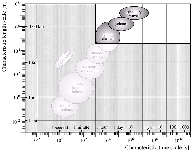
Figure 1. Distribution of atmospheric dynamical processes in the weather system, sorted according to spatial and temporal scales. The stippled part, with small scale processes, is usually not explicitly described in models of the system, but “parametrized.” von Storch and Zwiers (1999); ©Cambridge University Press.

This observation was the key for modern weather forecasting, as was expressed by Starr (1942):

“The General Nature of Weather Forecasting. The general problem of forecasting weather Conditions may be subdivided conveniently into two parts. In the first place, it is necessary to predict the state of motion of the atmosphere in the future; and, secondly, it is necessary to interpret this expected state of motion in terms of the actual weather which it will produce at various localities. The first of these problems is essentially of a dynamic nature, inasmuch as it concerns itself with the mechanics of the motion of a fluid. The second problem involves a large number of details because, under exactly similar conditions of motion, different weather types may occur, depending upon the temperature of the air involved, the moisture content of the, air, and a host of, local influences'.”

First ideas along the lines of this article were presented in a conference proceeding by Von Storch (1999).

It may be useful to define, what we mean with the word “downscaling,” and the “attributes” empirical” and “dynamical.” The basic idea of downscaling is the observation that in amny case, the statistics of variables of interest at smaller scales may be skillfully estimated by relating it to the state of larger scales. Thus, the state of large sclaes becomes the “predictor,” or maybe better: the “conditioner” of the smaller scale statistics. The downscaling is empirical, when the link is empirically determined, in particular by fitting statistical models; it is dynamical, when the link is established by process-based models, in particular limited area models of the hydro- and thermodynamics of the atmosphere or the ocean. The main focus of our article is on the empirical part, but the dynamical one is also dealt with.

The purpose of this article is to present the roots of ideas, which were used to build the concept of downscaling, namely synoptic climatology and spatial interpolation. As such, the article dos not present new ideas of how to do downscaling, nor an improved systematic of the various avenues available to do downscaling. Instead it is an account of the history of ideas behind something like an “industry” in climate sciences, which began with first publications in the early 1990s, but exploited earlier work, such as that of the above-mentioned Victor Starr.

The technical aspects of implementing downscaling is subject to books and articles in encyclopedias, as will is listed below.

Empirical Procedures

The term “downscaling” was introduced by von Storch et al. (1991)—it refers to a statistical approach that relates statistics of large scales to statistics of small scales, or impacts

with small scale climate states $S_t^C$, large-sale climate states $L_t^C$, and small-scale physiographic details ${\eta }_t^S$, which are external to the dynamics. The superscript C refers to “climate,” and F represents a statistical model. This model, possibly based on a phenomenological motivation, is fitted to recorded samples of the statistics of the large scales and the small scales (or impacts). F can take various forms, but it is always a kind of interpolated map, with L${}_t^C$ as coordinates (more on this later). The time t is no longer a time instance, but represents monthly or annual means. For early reviews, refer to von Storch et al. (2000a) or Zorita and von Storch (1997).

The link (2) is not a direct dynamical link, i.e., it may be that the large-scale “predictor,” say the monthly mean intensity of westerly, has nothing directly to do with the forming of the state of the predictand, such as the height of storm surges at a certain location. Instead the link exploits the empirically derived fact that in months with on average stronger westerly winds, higher storm surges are observed in Cuxhaven (by referring to a later example). The main wind does nothing with the water, but embedded in an intensified westerly wind, more and heavier storms travel. And these, the embedded storms, cause the accumulation of coastal waters (von Storch and Reichardt, 1997).

This indirect statistical link can be more explicitly resolved by including in S${}_t^C$ not only the expected mean of the small-scale variables (conditioned on the large-scale flow), but instead parameters that describe a full probability distribution or a stochastic process. These parameters are the ones that are conditioned on the large-scale dynamics (Wilby et al., 1999, 2002; Busuioc and von Storch, 2003).

In the following sections The Interpolation Problem and Example: Fitting surfaces, we address and illustrate the concept of extending a cloud of data into a mapping, in case of a 2-dimensional problem a surface, by interpolation. Before doing so we discuss the closely related concept of dynamical downscaling.

Dynamical Procedures

Empirical downscaling is related to dynamical downscaling, which grew from limited area modeling. However, in the conventional set-up this latter procedure is nor really “downscaling,” i.e., deriving estimates of smaller-scale states from larger-sale states, but all scales along a lateral boundary zone. The introduction of large-scale constraints overcame this limitation, and allowed eventually global dynamical downscaling.

This principle describes downscaling “weather.” In a formal nutshell, it may be expressed as

With the large-scale weather state L${}_t^w$, the small-scale weather state S${}_{t,}^w$ and some physiographic details ${\eta }_t^s$ at small scales, which are external to the dynamics. M represents a dynamical model.

A “climate” downscaling may be obtained by applying the model (2) repeatedly to a sufficiently large number of large-scale states, which sample the “climate” (the statistics of weather) sufficiently completely.

In a pure form, this concept was implemented by the stochastic-dynamic method [SDM; e.g., (Frey-Buness et al., 1995)], which ran a limited area model covering, for instance, the Alps with a set of characteristic weather variables, such as wind direction or vertical stability. This approach was computationally efficient, as a large number of (short term) simulations were feasible, even if a very high resolution was as implemented.

Later this concept was replaced by running regular “limited area models” (LAM, Dickinson et al., 1989), originally derived from regional atmospheric forecast models. These models, forced along the lateral boundaries with time-variable atmospheric states (and lower boundary values), were run for sufficiently long time, so that statistics could be derived from the small-scales simulated by the LAM. The LAMs replaced the SDM method after more and more computing time became available, and the heavy computational costs needed for running LAMs for extended times became affordable.

Dynamical downscaling has been studied and extensively pursued in big internationally coordinated projects, such as the the European projects PRUDENCE (Christensen et al., 2002) and ENSEMBLES (Christensen et al., 2007) or the international CORDEX (Giorgi and Gutowski, 2015; Souverijns et al., 2019).

In the beginning the LAM method was not labeled as “downscaling,” and indeed it does not represent a downscaling in a strict sense—the model does not process given large-scale states, but all scales along a narrow boundary (“sponge”) zone. A consequence is that the state in the interior is not uniquely determined by the boundary values—a mathematical fact long known. If the area is relatively small, and the region is well-flushed (i.e., disturbances travel quickly through the region, as is the case with most mid-latitude regions), multiple solutions rarely emerge. However, if the region is large, say covering the entire contiguous US, then the steering of the interior state by the boundaries becomes weak (Castro and Pielke, 2004) and the model shows often tendencies of “divergence in phase space.”

Much later, a truly downscaling methodology was developed by introducing a large-scale constraint (e.g., scale-dependent spectral nudging; Waldron et al., 1996; von Storch et al., 2000b) into the LAMs; with this modification, the model was no longer used to solve a boundary value problem but as a data assimilation scheme, which blended dynamical knowledge (the equations of motions etc.) with empirical knowledge (the large-scale state). The success of doing so was illustrated by the case of the contiguous US (Rockel et al., 2008).

Even later, the obvious extension of using the large-scale constraint in a global model (Yoshimura and Kananitsu, 2008; Schubert-Frisius et al., 2017; von Storch et al., 2017) was implemented, which then generates details in all regional states, consistently with the large-scale (global) state. This cannot be done with regular unconstrained global models (GCMs), because there is no way of enforcing a particular large-scale state. This illustrates that conventional unconstrained LAMs are not really “downscaling.”

State of the Art

Downscaling has become a household term and hardly needs an explanation when used in scientific papers and reports. Encyclopedias, as well as similar collections of articles, feature accounts of the concept and issues (Rummukainen, 2009, 2015; Wilks, 2010; Ekström et al., 2015; Benestad, 2016), and books have been published (Benestad et al., 2008; Maraun and Widmann, 2018).

While (2) describes “weather downscaling,” in most cases by exploiting dynamical models, the relationship (1) represents “climate downscaling,” which by using empirical links relates a predictand to a predictor. The advantage of methods based on (2) is that they may be better for studying so far unobserved states, assuming that the considered processes describe the dynamics of the unobserved states well, while (1) allows building links between variables which can hardly be linked dynamically, such as winter mean temperatures and the timing of flowering of a plant (Maak and von Storch, 1997).

The Interpolation Problem

Today, we are used to present spatial distributions as geographical maps, implicitly assuming that we would have data at all locations—but we have only data at some locations; the rest is achieved by spatial interpolation. It was Alexander von Humboldt, who pioneered this practice in 1817 (e.g., Knobloch, 2018). Humboldt himself saw the introduction of the concept as one of his major achievements (details: Knobloch, p. 21). He explained in a 1853 book: “Kann man verwickelte Erscheinungen nicht auf eine allgemeine Theorie zurückführen, so ist es schon ein Gewinn, wenn man das erreicht, die Zahlen-Verhältnisse zu bestimmen, durch welche eine große Anzahl zerstreuter Beobachtungen miteinander verknüpft werden können, und den Einfluß lokaler Ursachen der Störung rein empirischen Gesetzen zu unterwerfen.“¹ (Humboldt 1853, S. 207; quoted after Knobloch, 2018).

Humboldt named these lines “isotherms.” Von Storch (1999) noted: “These contour lines chiefly served the purpose of visualizing the quantitative data. Inside the 20 degree isotherm all stations report temperature larger than 20 degrees, whereas outside the area enclosed by this isoline the temperature at all stations would be less than 20 degrees. The isotherm itself is imaginary; in principle there is such a line, but it can be determined only approximately; it is the art of spatial interpolation to describe this unknown unobservable line.”

Obviously, the concept can, and was generalized to show “isolines” of other geophysical quantities, such as frequency of winds with gale speeds or amounts of rainfall. Prominent names were Vladimir Köppen and his coworker Rudolf Geiger, who presented their climate classification maps in this way.

However, when more and more mathematical thinking spread in the scientific community, the link to geographical maps weakened, and more general coordinates were introduced. Von Storch (1999) introduced as an example Osborn's et al. (1999) analysis of precipitation in Central England given as a function of vorticity and flow direction (Figure 2). We use this example here not because of specific physical interest—this has been dealt with in the original paper by Osborn et al. (1999)—but because it allows to transparently and imply illustrate the issues.

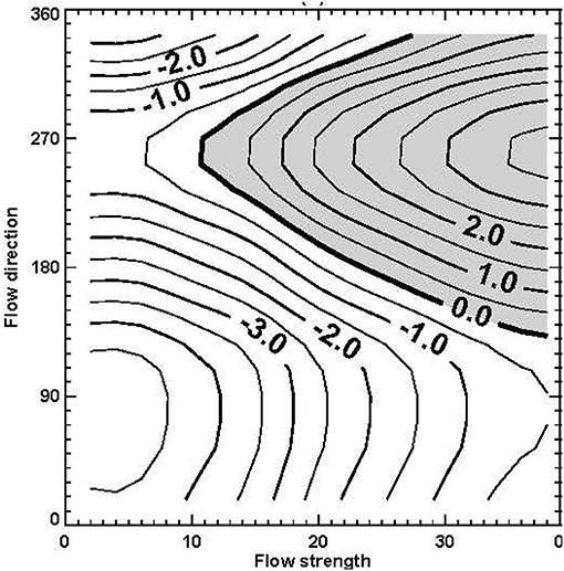
Figure 2. Mean precipitation anomalies (i.e., deviations from the long term mean; in mm/day) in Central England given as function of flow direction (degree) and flow strength (m/s). From Osborn et al., 1999; © Inter-Research 1999.

Of course, continuously distributed data did not exit for preparing this map; instead the limited number of scattered data points were binned into a finite number of boxes, and after interpolation isolines were plotted. Figure 2 informs that a value of −2.5 mm/day for flow strength of 20 m/s and a flow direction of 100° is the mean anomaly (difference from long term mean) of precipitation amounts across all available reports on days with a flow strength of about 20 m/s and a flow direction of about 100°.

Figure 2 shows a 2-dimensional representation, as geographical maps do. But once more general coordinates were introduced, the generalization to more dimensions became possible (even though the graphical presentation is lost, when four and more dimensions are employed).

Von Storch (1999) formalized the concept by asking for an interpolation of K data points, labeled as G^k at “locations” x^k = (x${}_1^{\text{k}}$, … x${}_{\text{n}}^{\text{k}}$) in an n-dimensional space. The result of the interpolation is a “surface” I, with values for all points x = (x₁, … x_n) in the n-dimensional space, with the property that the difference of this surface at the given data points is limited by some values, say || I(x^k)—G^k || < δ. The maximum accepted deviation δ is in most cases zero. In case of kriging, when a “nugget effect” is considered, δ may is non-zero (Wackernagel, 1995).

Implicitly it is assumed that there is a “true” surface I, with accurate manifestations G^k = I(x^k) at the locations x^k. This is meaningful in traditional geographical problems, but in some cases G^k may be considered a random realization of I(x^k)—for instance, when the data are collected during different times, and the distribution varies in randomly in time. Then I may represent the localized expectation of G, i.e., I(x) = E(G|x), with the expectation operator E.

In Figure 2 Middle England precipitation is presented as being determined by direction and strength, but there are certainly other factors—thus, precipitation is not determined by the two considered factors, but conditioned, in a stochastic sense.

Von Storch (1999) notes that “the result of the interpolation is an approximate or estimated surface I_E, which differs to some extent from the “true” surface of conditional expectations. The purpose of the spatial interpolation is the determination of the surface I(x) and not the reproduction of the points G_k. Therefore, the success of I_E as an estimator of I may be determined only by comparing the estimates I_E(x) with the additional G(x)-values at a number of data points x, which have not been used in the estimation process.”

Example: Fitting Surfaces

The question is how such surfaces may be constructed. The interpolation itself can be done in various ways; they differ with respect to a-priori assumptions made about the structure of the surface.

The strongest assumption specifies the global structure. A frequent case refers to multiple regression, which suggests that the surface is a (linear) plane. Often the regression is based on Canonical Correlation Analysis or Redundancy Analysis (cf. von Storch and Zwiers, 1999).

If the assumption deals only with local properties, the fitting process is considerably more flexible. Straight forward linear interpolation is an example; Brandsma and Buishand (1997) have used cubic splines for specifying precipitation as a function of temperature. Osborn's example (Figure 2) belongs also to this class of interpolations. Geostatistical interpolation, often simply called kriging, is a widely used in mathematical geosciences (e.g., Harff and Davis, 1990), which has also be used for downscaling (e.g., Biau et al., 1999). Fashionable approaches such as neural networks (e.g., Chadwick et al., 2011) and fuzzy logic (e.g., Faucher et al., 1999; Bardossy et al., 2005) are also in use.

The analog, or nearest neighbor, (Zorita et al., 1995; Brandsma and Buishand, 1998; Zorita and von Storch, 1999) represents the surface as piecewise constant plateaus around the data. In geostatistical cricles the method is also known as Voronoi nets (cf. Stoyan et al., 1997).

For illustration, we discuss here three different approaches—bivariate regression, ordinary kriging, and analog—using an example of generalized coordinates in a phase space. We have chosen this example to illustrate that rather abstract problems may be considered.

When preparing a spatial interpolation, some assumptions about the data G at locations x need to be made. The major assumption is that G is representative for a neighborhood of x, or that I has the same statistical properties in that neighborhood. A correlation length scale may be representative for this neighborhood; this is explicitly so in case of kriging. In that concept, also some spatial discontinuities are permitted (“Nugget effect”; Wackernagel, 1995).

The example employs the displaying the mean summer seasonal cyclonic eddy diameters in the South China Sea (Zhang and von Storch, 2018) as a function of the coefficients of indices of the regional barotropic stream function (the stream function of the vertically averaged flow). Both, the eddy properties as well as the stream function have been constructed using a dynamical ocean model, which was forced with variable atmospheric conditions for the 61 summer seasons 1960–2010 (Zhang and von Storch, 2018). Obviously, the case presented here has no specific significance for the presentation here; it is a mere example, which demonstrates how different interpolating surfaces may be constructed.

The dynamical concept is that some statistics of migrating ocean eddies, in this case the mean seasonal size, may be related to variations in the current patterns. Of course, not all variations in eddy size can be traced back to current anomalies but it is reasonable to suggest that eddy size may be seens as a random variable conditioned upon the prevailing currents.

As predictors we use the barotropic stream function In the South China Sea, which is given at 57,750 locations; such large dimension cannot be handled, and therefore the dimension of the problem is reduced in this discussion—to 2. The needed two indices are chosen to be coefficients of the leading Empirical Orthogonal Functions (EOFs; for a detailed introduction, refer to Preisendorfer, 1988; von Storch and Zwiers, 1999) or principal components of the barotropic stream function field. EOFs are a system of orthogonal vectors which are adapted to be most powerful in representing variance of the considered variable, which is here the barotropic streamfunction of the entire South China Sea.

The two indices represent 31.5 and 10.5% of the dominant interannual variations of the barotropic stream function (Figure 3).

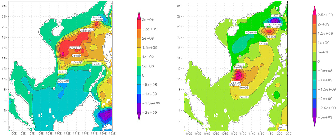
Figure 3. Dominant patterns of interannual variability of summer season barotropic stream function in the South China Sea, the coefficients of which are used in the presentation in Figure 4 and in the mapping efforts shown in Figure 5. Currents follow the gradients of the stream function, clockwise around a center of high (red) values, and counterclockwise around centers with negative (blue) values. Unit: kg s⁻¹ (kg/s). Courtesy: Zhang Meng.

The seasonal mean diameters of cyclonic eddies in the South China Sea are displayed in Figure 4 as a function of these first two EOF coefficients; for each summer season (June-August) one dot is plotted, with the vertical coordinate indicting the diameter in km. Obviously the eddy diameters do not constitute a smooth surface; this is meaningful when we consider formation and the intensification of eddies all as a conditional random variable, and each observed mean eddy diameter is considered one realization of a conditional random variable.

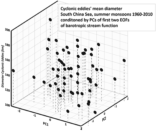
Figure 4. Seasonsal means of cyclonic eddies' diameter in the South China, 1960–2010, given as function of the principal components of the first two EOFs of the barotropic stream function in the South China Sea as shown in Figure 3.

We have applied three different interpolation techniques to the anomalies (i.e., deviations from the long term mean) derived from the data displayed in Figure 4; the results are shown as “isolines” in Figure 5 The three techniques are bilinear regression (top left) and nearest neighbors (analog; top right), and ordinary kriging (bottom).

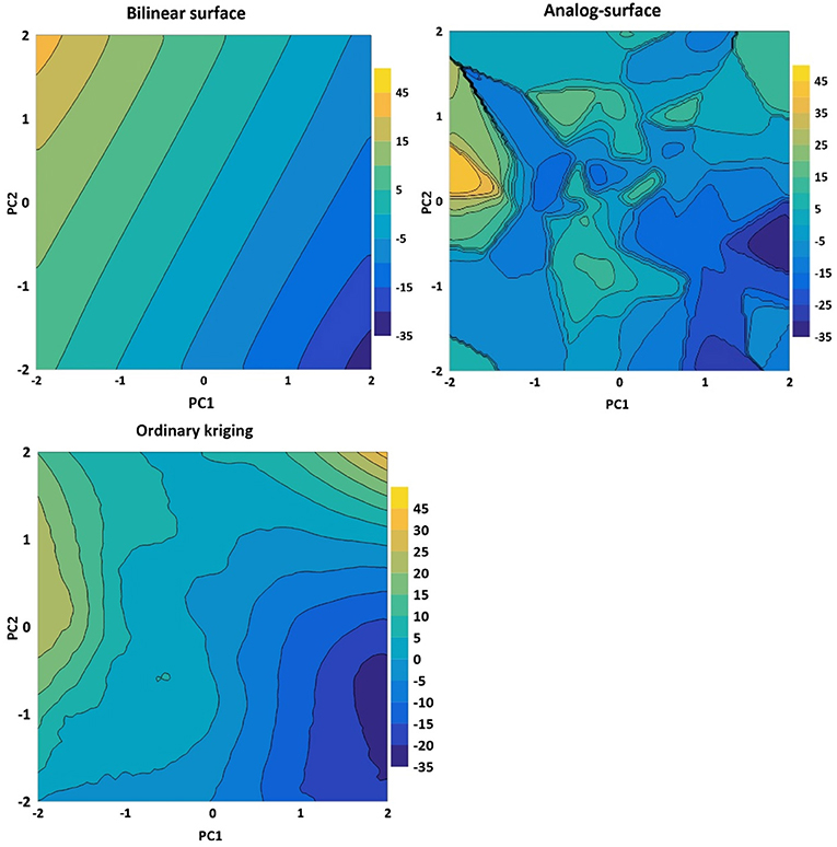
Figure 5. Interpolation of the data points shown in Figure 4 by means of bivariate regression, by an analog approach, and by ordinary kriging. The coordinates are the principal components of the first two EOFs of the barotropic stream function, shown in Figure 3.

Kriging is a methodology which was developed in geology for mapping structures. At this time, details do not matter so that it may suffice to mention that “ordinary kriging” was used, employing a linear Matheron function and allowing for a nugget effect (cf., Wackernagel, 1995; Maciag, pers. comm.)

The numbers describe the deviation from the overall mean. The two methods of the bivariate regression and of the nearest neighbor are at the opposite ends of complexity. The bilinear regression is smooth, with less variability. The analog, on the other hand, is very noisy, with rather large abrupt changes, but with a variability which reproduces the variability of the original data, say in terms of variability and skewness, while the krigged surface contains elements of the two other maps, but has a richer structure than the bivariate surface, and is less noisy than the analog-based map. As expected, the krigged map is between the other two, in terms of smoothness and noise.

Seemingly there is no way of deciding which of three maps is “better”; they share a certain basic structure, with high values near the upper left corner, and lower values in the lower right corner. Which map will eventually be chosen depends on how the map will be used. If a general overview is needed, the bivariate may be best; if it is used for weather generators, the analog may be the choice. If details matter, the richer but smooth structure of kriging may be more favorable.

In terms of the link to the barotropic stream function (Figure 3), we find the size of cyclonic eddies larger, when both (EOF) patterns prevail in a season, i.e., when there resides an anomalous large and stationary anticyclone in almost the entire northern part of the South China Sea (combination of patterns 1 and 2), and an anomalous outward flow through the Luzon strait. In the same way, smaller eddies are generated on average, when an anomalous counterclockwise flow streams through the South China Sea. Pattern 1 alone goes also with these characteristics, but is associated with a weaker signal, when EOF2, the second pattern, does not contribute. The same holds for pattern 2 in the absence of pattern 1, but with an even weaker signal.

Discussion: Application of a Map in Downscaling

As mentioned before, the thinking about downscaling is rooted in two different concepts, one in meteorology named “synoptic climatology,” the other in “interpolation of data clouds,” which was inspired by spatial interpolation.

The basic idea, as introduced the first time likely by Kim et al. (1984), and later by von Storch and Zorita (1990), recognized the limitation of climate modeling, in particular construction of climate change scenarios, in representing small scale phenomena, and many aspects of impacts of climate variability and change.

The aspect of synoptic climatology was employed in the “statistical dynamical method,” and was based on building causal (process-based) links between a conditioning large-scale state and a resulting small-scale response; later this method became less and less popular when dynamical downscaling matured and—given the advances of computational power—allowed the simulation of continuous sequences of large-scale forcing.

The other aspect, however, the “interpolation of data clouds,” is still in use—it makes use of co-variations, which are not necessarily based on direct causal links. Instead the links may be indirect, such as the emergence of extreme values in a season and the mean state during that season—obviously the mean state does not “make” extremes, but the mean state may favor the formation of synoptic situations which lead to extremes (cf., Branstator, 1995). The example presented in this paper, on the formation of large vortices in the South China Sea, conditioned by mean currents, falls into this category.

Such efforts result in tables, or in maps, which suggest a state of a small-scale or an impact variable, conditional upon some adopted large-scale indicators. When two such variables are used, then the result takes the form of a table, and the method curtails an interpolation, a map-generating effort. The purpose of interpolation is “to guide people in unknown terrain” (Von Storch, 1999), i.e., to guess the state of the system at “locations” not visited no far. Such guesses can be of very different format, depending on the user's needs.

In general, at each point, the method would return a probability interval I_E(x) ± Δ, with I_E(x) representing the conditional expectation and Δ a level of uncertainty (say, two standard deviations). In many cases, however, only the conditional expectation will be provided (in the bilinear regression case), whereas sampling from the analog-map will result in random samples including the variability. Thus, the former will be favorable, when dealing with typical conditions, whereas the second gives noisy numbers, but with the right level of variability, as needed in weather generators (cf. Zorita et al., 1995).

Author Contributions

All authors listed have made a substantial, direct and intellectual contribution to the work, and approved it for publication.

Conflict of Interest Statement

The authors declare that the research was conducted in the absence of any commercial or financial relationships that could be construed as a potential conflict of interest.

Acknowledgments

We thank Łukasz Maciag of the Institute of Marine and Coastal Sciences of the University of Szczecin, Poland, Jan Harff of the University of Sczcecin, Poland, Zhang Meng of the Institute of Coastal Research in Geesthacht, Tim Osborn of Climate Research Unit (CRU) in Norwich and Alexander Kolovos. ŁM prepared the kriging map (Figure 5), while JH and AK helped with advice on this matter; Zhang Meng supplied us with the data of the example and with Figure 4, and Tim Osborn provided and allowed us the usage of Figure 2.

Footnotes

References

Bardossy, A., Bogardi, I., and Matyasovszky, I. (2005). Fuzzy rule-based downscaling of precipitation. Theor. Appl. Climatol. 82, 119–129. doi: 10.1007/s00704-004-0121-0
Benestad, R. (2016). Downscaling Climate Information. New York, NY: Oxford University Press Research Encyclopedia on Climate Science.
Benestad, R. E., Hanssen-Bauer, I., and Chen, D. (2008). Empirical-Statistical Downscaling. Hackensack, NJ: World Scientific Publishers.
Biau, G., Zorita, E., von Storch, H., and Wackernagel, H. (1999). Estimation of precipitation by kriging in EOF space. J. Climate 12, 1070–1085.
Brandsma, T., and Buishand, T. A. (1997). Statistical linkage of daily precipitation in Switzerland to atmospheric circulation and temperature. Hydrol. J. 198, 98–123.
Brandsma, T., and Buishand, T. A. (1998). Simulation of extreme precipitation in the Rhine basin by nearest neighbor resampling. Hydrol. Earth Sys. Sci. 2, 195–209.
Branstator, G. (1995). Organization of storm track anomalies by recurring low-frequency circulation anomalies. J. Atmos. Sci. 52, 207–226.
Busuioc, A., and von Storch, H. (2003). Conditional stochastic model for generating daily precipitation time series. Clim. Res. 24, 181–195. doi: 10.3354/cr024181
Castro, C.L., and Pielke, R. A. Sr. (2004). Dynamical downscaling: assessment of value restored and added using the Regional Atmospheric Modelling System. J. Geophys. Res. 110, 1–21. doi: 10.1029/2004JD004721
Chadwick, R., Coppola, E., and Giorgi, F. (2011). An artificial neural network technique for downscaling GCM outputs to RCM spatial scale. Nonlin. Processes Geophys. 18, 1013–1028. doi: 10.5194/npg-18-1013-2011
Christensen, J. H., Carter, T., and Giorgi, F. (2002). PRUDENCE Employs New Methods to Assess European Climate Change. EOS Transactions of the American Geophysical Union 83, 147.
Christensen, J. H., Christensen, O. B., Rummukainen, G., and M Jacob, D. (2007). “ENSEMBLES Regional Climate Modeling: a multi-model approach towards climate change predictions for europe and elsewhere,” in: American Geophysical Union, Fall Meeting 2007. Available online at: http://adsabs.harvard.edu/abs/2007AGUFMGC23B.01C.
Dickinson, R. E., Errico, R. M., Giorgi, F., and Bates, G. T. (1989). A regional climate model for the western United States. Clim. Change 15, 383–422.
Ekström, M., Grose, M. R., and Whetton, P. H. (2015). An appraisal of downscaling methods used in climate change research. WREs Clim. Change 6, 301–319. doi: 10.1002/wcc.339
Faucher, M., Burrows, W., and Pandolfo, L. (1999). Empirical-Statistical reconstruction of surface marine winds along the western coast of Canada. Clim. Res. 11, 173–190.
Frey-Buness, F., Heimann, D., and Sausen, R. (1995). A statistical-dynamical downscaling procedure for global climate simulations. Theor. Appl. Climatol. 50, 117–131.
Giorgi, F., and Gutowski, W. J. Jr. (2015). Regional dynamical downscaling and the CORDEX initiative. Annu. Rev. Environ. Resour. 40, 467–490. doi: 10.1146/annurev-environ-102014-021217
Harff, J., and Davis, J. C. (1990). Regionalization in geology by multivariate classification. Math. Geol. 22, 573–588.
Kim, J. W., Chang, J.-T., Baker, N. L., Wilks, D. S., and Gates, W. L. (1984). The statistical problem of climate inversion: determination of the relationship between local and large-scale climate. Mon. Wea. Rev. 112, 2069–2077.
Knobloch, E. (2018). “Zum Verhältnis von Naturkunde/Naturgeschichte und Naturwissenschaft. Das Beispiel Alexander von Humboldt,“ in Umgangsweisen mit Natur(en)in der Frühen Bildung III. Eds M. Rauterberg, and G. Scholz (Über Naturwissenschaft und Naturkunde). Available online at: www.widerstreit-sachunterricht.de Beiheft 12. 13–36.
Maak, K., and von Storch, H. (1997). Statistical downscaling of monthly mean air temperature to the beginning of the flowering of Galanthus nivalis L. in Northern Germany. Intern. J. Biometeor. 41, 5–12.
Maraun, D., and Widmann, M. (2018). Statistical Downscaling and Bias Correction for Climate Research. Cambridge: Cambridge University Press, 360 p.
Osborn, T. J., Conway, D., Hulme, M., Gregory, J. M., and Jones, P. D. (1999). Air flow influences on local climate: observed and simulated mean relationships for the United Kingdom. Clim. Res. 13, 173–191. doi: 10.3354/cr013173
Preisendorfer, R.W. (1988). Principal Component Analysis in Meteorology and Oceanography. Amsterdam: Elsevier. 426 p.
Rockel, B., Castro, C. L., Pielke, R.A. Sr, von Storch, H., and Leoncini, G. (2008). Dynamical downscaling: Assessment of model system dependent retained and added variability for two different regional climate models. J. Geophys. Res. 113:D21107. doi: 10.1029/2007JD009461
Rummukainen, M. (2009). State-of-the-art with regional climate models. WIREs Clim. Change 1, 82–96. doi: 10.1002/wcc.8
Rummukainen, M. (2015). Added value in regional climate modeling. WREs Clim. Change 7, 145–159. doi: 10.1002/wcc.378
Schubert-Frisius, M., Feser, F., von Storch, H., and Rast, S. (2017). Optimal spectral nudging for global dynamic downscaling. Mon. Wea. Rev. 145, 909–927. doi: 10.1175/MWR-D-16-0036.1
Souverijns, N., Gossart, A., Demuzere, M., Lenaerts, J. T. M., Medley, B., Gorodetskaya, I. V., et al. (2019). A new regional climate model for POLAR-CORDEX: evaluation of a 30-year hindcast with COSMO-CLM2 over Antarctica. J. Geophys. Res. Atmosphere. doi: 10.1029/2018JD028862. [Epub ahead of print].
Starr, V.P. (1942). Basic Principles of Weather Forecasting. New York,NY; London: Harper Brothers Publishers. 299 p.
Stoyan, D., Stoyan, H., and Jansen, U. (1997). Umweltstatistik: Statistische Verarbeitung und Analyse von Umweltdaten. Leipzig: Teubner Stuttgart. 348 p.
Von Storch, H. (1999). “Representation of conditional random distributions as a problem of “spatial” interpolation,” in geoENV II - Geostatistics for Environmental Applications, eds J. Gòmez-Hernàndez, A. Soares and R. Froidevaux (Dordrecht; Boston, MA; London: Kluwer Adacemic Publishers), 13–23.
von Storch, H., Feser, F., Geyer, B., Klehmet, K., Li, D., Rockel, B., et al. (2017). Regional re-analysis without local data - exploiting the downscaling paradigm. J. Geophys. Res. 122, 8631–8649. doi: 10.1002/2016JD026332
von Storch, H., Hewitson, B., and Mearns, L. (2000a). “Review of empirical downscaling techniques, “Regional Climate Development Under Global Warming, eds T. Iversen, and B. A. K. Høiskar (Torbjørnrud: General Technical Report No. 4. Conf. Proceedings RegClim Spring Meeting Jevnaker), 29–46.
von Storch, H., Langenberg, H., and Feser, F. (2000b). A spectral nudging technique for dynamical downscaling purposes. Mon. Wea. Rev. 128, 3664–3673. doi: 10.1175/1520-0493(2000)128 < 3664:ASNTFD>2.0.CO;2
von Storch, H., and Reichardt, H. (1997). A scenario of storm surge statistics for the German Bight at the expected time of doubled atmospheric carbon dioxide concentration. J. Climate 10, 2653–2662.
von Storch, H., and Zorita, E. (1990). Assessment of regional climate changes with the help of global GCM's: an example. CAS/JSC Working group on Numerical Experimentation. WMO Report no. 14, 7.30.
von Storch, H., Zorita, E., and Cubasch, U. (1991). Downscaling of global climate change estimates to regional scales: an application to Iberian rainfall in Wintertime. MPI Rep. 62:36.
von Storch, H., and Zwiers, F. W. (1999). Statistical Analysis in Climate Research. Cambridge: Cambridge University Press. 528 p.
Waldron, K. M., Peagle, J., and Horel, J. D. (1996). Sensitivity of a spectrally filtered and nudged limited area model to outer model options. Mon. Wea. Rev. 124, 529–547.
Wilby, R.L., Dawson, C. W., and Barrow, E. M. (2002). SDSM — a deci-sion support tool for the assessment of regional climate change impacts. Environ Model Softw. 17, 145–157. doi: 10.1016/S1364-8152(01)00060-3
Wilby, R.L., Hay, L. E., and Leavesley, G. H. (1999). A comparison of downscaled and raw GCM output: implications for climate change scenarios in the San Juan River Basin, Colorado. J Hydrol. 225, 67–91.
Wilks, D.S. (2010). Use of stochastic weathergenerators for precipitation downscaling. WIREs Clim. Change 1, 898–907. doi: 10.1002/wcc.85
Yoshimura, K., and Kananitsu, M. (2008). Dynamical global downscaling of global reanalysis. Mon. Wea. Rev. 136, 2983–2998. doi: 10.1175/2008MWR2281.1
Zhang, M., and von Storch, H. (2018). Distribution features of travelling eddies in the South China Sea. Res. Activit. Atmosph. Oceanic Model. 2–31.
Zorita, E., Hughes, J., Lettenmaier, D. P., and von Storch, H. (1995). Stochastic characterization of regional circulation patterns for climate model diagnosis and estimation of local precipitation. J. Clim. 8, 1023–1042.
Zorita, E., and von Storch, H. (1997). A Survey of Statistical Downscaling Techniques. Geesthacht: GKSS 42 p.
Keywords: downscaling, spatial interpolation, synoptic dynamics, history of ideas, empirical downscaling
Citation: von Storch H and Zorita E (2019) The History of Ideas of Downscaling—From Synoptic Dynamics and Spatial Interpolation. Front. Environ. Sci. 7:21. doi: 10.3389/fenvs.2019.00021
Received: 24 September 2018; Accepted: 05 February 2019;
Published: 26 February 2019.
Edited by:
Raquel Nieto, University of Vigo, SpainReviewed by:
Kei Yoshimura, The University of Tokyo, JapanEnrique Sanchez, University of Castilla La Mancha, Spain
Copyright © 2019 von Storch and Zorita. This is an open-access article distributed under the terms of the Creative Commons Attribution License (CC BY). The use, distribution or reproduction in other forums is permitted, provided the original author(s) and the copyright owner(s) are credited and that the original publication in this journal is cited, in accordance with accepted academic practice. No use, distribution or reproduction is permitted which does not comply with these terms.
*Correspondence: Hans von Storch, hvonstorch@web.de