


Abstract
The Parker Solar Probe (PSP) completed its first solar encounter in 2018 November, bringing it closer to the Sun than any previous mission. This allowed in situ investigation of the heliospheric current sheet (HCS) inside the orbit of Venus. The Parker observations reveal a well defined magnetic sector structure placing the spacecraft in a negative polarity region for most of the encounter. The observed current sheet crossings are compared to the predictions of both potential field source surface and magnetohydrodynamic models. All the model predictions are in good qualitative agreement with the observed crossings of the HCS. The models also generally agree that the HCS was nearly parallel with the solar equator during the inbound leg of the encounter and more significantly inclined during the outbound portion. The current sheet crossings at PSP are also compared to similar measurements made by the Wind spacecraft near Earth at 1 au. After allowing for orbital geometry and propagation effects, a remarkable agreement has been found between the observations of these two spacecraft underlying the large-scale stability of the HCS. Finally, the detailed magnetic field and plasma structure of each crossing is analyzed. Marked differences were observed between PSP and Wind measurements in the type of structures found near the HCS. This suggests that significant evolution of these small solar wind structures takes place before they reach 1 au.
Export citation and abstract BibTeX RIS
1. Introduction
The interplanetary magnetic field (IMF) is organized into two hemispheres, or sectors where the magnetic field lines have a direction either away or toward the Sun (Wilcox & Ness 1965). The boundary separating these two sectors is called the heliospheric current sheet (HCS). It has long been established that the HCS is the interplanetary extension of the solar neutral line (Schulz 1973) and that it is a warped surface with a latitudinal extent that varies with solar cycle (Smith et al. 1978, 1993; Klein & Burlaga 1980; Thomas & Smith 1981; Hoeksema et al. 1983; Lepping et al. 1996).
On a smaller scale, the structure of the HCS and its vicinity is less understood. Near 1 au, the traversal of a spacecraft from one magnetic polarity to another typically involves the crossings of multiple large magnetic field discontinuities of ∼180° field rotations often assumed to correspond to the multiple crossing of a single, wavy current sheet (Behannon et al. 1981; Lepping et al. 1996). Crooker et al. (1993) interpreted the same observations as a network of individual current sheets emanating from different helmet streamers.
In addition to magnetic field measurements, directional heat flux signatures in the suprathermal component of solar wind electrons (i.e., strahl), which generally stream away from the Sun along the magnetic field lines (Feldman et al. 1975), have been successfully used to shed new light on the nature of HCS crossings. At true sector polarity reversals the magnetic field changes its direction from inward to outward or vice versa while the strahl electrons continue to stream away from the Sun. This results in a 180° shift in the strahl electron pitch angle distribution (PAD), or the relative direction between the electron flow and magnetic field lines (or heat flux direction). For many of the large magnetic field rotations associated with the HCS, no such PAD changes were observed (Kahler et al. 1996; Szabo et al. 1999a, 1999b) and thus are not true HCS crossings but indicate the presence of other magnetic structures nearby. Recently, Sanchez-Diaz et al. (2017, 2019) argued that stream blobs observed in white light coronagraph data continue to stream out into the heliosphere along the HCS and are observable in situ as small solar wind density enhancements and small magnetic field flux ropes depending on the timing of the HCS crossing, uniting the different features observed by Wind and Helios into a single picture.
In this paper, we analyze the Parker Solar Probe (PSP) observations of the HCS made during the first solar encounter between 2018 October 6 and December 6. The general properties of the data are described in Section 2, and the observed HCS crossing times and locations are compared to model predictions in Section 3. Section 4 compares the PSP observations of the HCS to similar measurements made by the Wind spacecraft near Earth. Lastly, the small-scale structure of the HCS near the Sun is discussed in Section 5 with a summary offered in Section 6.
2. Parker Solar Probe Observations
The PSP project was able to return measurements from the probe not only from the encounter time period, when the spacecraft was within 0.25 au of the Sun, but almost all the way to the orbit of Venus. Figure 1 shows PSP observations between 2018 October 6 and December 6. The bottom panel shows the radial distance from the Sun covered by PSP during this time. The middle panels depict the magnetic field observed in RTN spherical coordinates where the azimuth angle (ϕB) is zero in the radial direction away from the Sun, and the latitude angle (θB) is positive north of the ecliptic (Bale et al. 2016). The increasing magnetic field strength as the spacecraft approaches the Sun is evident. The top two panels show the 315 eV heat flux electron PADs in flux units and normalized, where normalization was carried out for each time step removing the flux variability (Kasper et al. 2016, 2019). The positive and negative magnetic field polarities, or away and toward sectors can be identified in the magnetic field azimuth angle data. Most of the large field rotations or sector changes are associated with electron PAD changes, indicating that the strahl suprathermal electrons are streaming along or antiparallel to the magnetic field lines. Eight regions of HCS crossings have been identified many composed of a sequence of substructures to be discussed in detail in Section 5. The time of the individual HCS crossings are listed in Table 1. Within 0.25 au, PSP traveled exclusively in a negative magnetic polarity region, and all of the observed HCS crossings are further outward from the Sun. However, these HCS encounters are still the closest ones to the Sun ever observed. In particular, the first HCS crossing in group #6 at 0.28404 au is the closest to the Sun ever observed.

Figure 1. PSP observations during the first solar encounter. The panels from top to bottom are 315 eV electron PAD, normalized 315 eV electron PAD, magnitude of the magnetic field, azimuth, and polar angles of the magnetic field in RTN coordinates, PSP radial distance from the Sun. Vertical dotted lines mark the HCS crossing regions.
Download figure:
Standard image High-resolution imageTable 1. HCS Crossings Observed by PSP
| Region | UT Start | Time | Duration | Radial | Polarityb | Event Typec |
|---|---|---|---|---|---|---|
| ID#a | (YYYY-mm-dd) | (hh:mm:ss) | (hh:mm:ss) | Distance (au) | ||
| Inbound | ||||||
| 1 | 2018 Oct 9 | 18:52:37 | 02:01:17 | 0.65 | +/+ | STR, MFD, eHFD, HDR? |
| 1 | 2018 Oct 9 | 22:06:38 | 02:05:08 | 0.65 | +/− | STR, MFS, eStrD, HDR? |
| 1 | 2018 Oct 10 | 03:48:14 | 06:35:55 | 0.64 | −/− | STR, MFD, eStrD, HDR? |
| 2 | 2018 Oct 18 | 04:40:22 | 00:00:02 | 0.52 | −/+ | HCS, Rec |
| 3 | 2018 Oct 20 | 08:24:48 | 01:54:54 | 0.48 | +/− | STR, MFD, eHFD |
| 4 | 2018 Oct 28 | 03:01:19 | 09:03:31 | 0.32 | −/+ | STR, MFD , FR, HDR? |
| 5 | 2018 Oct 29 | 10:49:42 | 00:23:13 | 0.30 | +/+ | STR, MFD, eHFD |
| 5 | 2018 Oct 29 | 13:01:30 | 02:54:28 | 0.29 | +/− | STR, MFD, eStrD, HDR? |
| Outbound | ||||||
| 6 | 2018 Nov 13 | 07:12:25 | 03:07:09 | 0.28 | −/+ | VMF, FR?, Rec |
| 6 | 2018 Nov 13 | 12:02:32 | 00:01:33 | 0.29 | +/− | HCS, eStrD, MFD |
| 6 | 2018 Nov 13 | 13:05:36 | 00:04:44 | 0.29 | −/+ | HCS, eStrD, MFD |
| 6 | 2018 Nov 13 | 13:38:57 | 00:03:34 | 0.29 | +/− | HCS, MFD |
| 6 | 2018 Nov 13 | 13:05:36 | 00:33:21 | 0.29 | −/− | STR |
| 6 | 2018 Nov 13 | 16:21:31 | 13:30:34 | 0.30 | −/+ | eStrD, VMF, FR?, Rec |
| 6 | 2018 Nov 14 | 11:12:53 | 06:38:21 | 0.31 | +/+ | VMF, Rec |
| 7 | 2018 Nov 23 | 18:27:03 | 00:12:13 | 0.50 | +/− | STR, MFD, Rec |
| 8 | 2018 Dec 6 | 00:07:01 | 00:57:01 | 0.68 | −/+ | FR? |
| 8 | 2018 Dec 6 | 05:36:40 | 00:04:27 | 0.68 | +/− | HCS, MFD |
| 8 | 2018 Dec 6 | 07:06:45 | 00:01:15 | 0.68 | −/+ | HCS, MFD |
| 8 | 2018 Dec 6 | 07:23:36 | 00:00:29 | 0.68 | +/− | HCS |
| 8 | 2018 Dec 6 | 07:47:02 | 00:00:32 | 0.68 | −/+ | HCS |
| 8 | 2018 Dec 6 | 08:39:30 | 00:00:32 | 0.68 | +/− | HCS |
| 8 | 2018 Dec 6 | 09:19:59 | 00:00:06 | 0.68 | −/+ | HCS, MFD |
| 8 | 2018 Dec 6 | 10:13:44 | 01:25:20 | 0.69 | +/+ | FR |
Notes.
aOne of the eight HCS crossing regions identified in the PSP data. Many HCS regions are composed of multiple substructures enumerated in this table. bMagnetic polarity of the region before and after the event. cCharacteristics of the event: HCS—single rapid crossing of current sheet, eStrD—electron strahl dropout, STR—stream with increased flow speed, MFD—magnetic field depression, HDR—high density region, FR—flux rope, VMF—variable magnetic field, Rec—reconnection jet.Download table as: ASCIITypeset image
3. Model Predictions of the HCS Geometry
The PSP observations provide the times of the HCS crossings, but global heliospheric models are needed to determine the global geometry of the HCS, and thus the angular distance of PSP from the HCS at any given time. This information is essential to assess the source region of the solar wind observed by PSP. We have employed two types of heliospheric models: potential field source surface (PFSS; Altschuler & Newkirk 1969; Schatten et al. 1969; Wang & Sheeley 1992) and magnetohydrodynamic (MHD; Steinolfson et al. 1975; Pizzo & Gosling 1994; Linker et al. 1999) simulations.
3.1. PFSS Model Predictions
The Wang–Sheeley–Arge (WSA) model (Arge & Pizzo 2000; Arge et al. 2003, 2004) is a combined empirical and physics based model of the corona and solar wind. It is an improved version of the original Wang and Sheeley model (Wang & Sheeley 1992). WSA uses ground-based line-of-sight (LOS) observations of the Sun's surface magnetic field, in the form of synoptic maps, as its input. In this work, we use global synchronic photospheric field maps generated by the Air Force Data Assimilative Photospheric Flux Transport (ADAPT; Arge et al. 2010, 2011, 2013; Hickmann et al. 2015) model. The ADAPT model utilizes flux transport, based on the Worden & Harvey (2000) model, to account for differential rotation, along with meridional and supergranulation flows, when observational data are not available. In addition, ADAPT incorporates new magnetogram input using the ensemble least-squares data assimilation technique to account for both model and data uncertainties as the maps are generated (Hickmann et al. 2015). For example, ADAPT heavily weights observations taken near the central meridian where magnetograms are most reliable, while the model specification of the field is generally given more weight near the limbs where observations are the least reliable. Since ADAPT is an ensemble model, a range of possible states (i.e., realizations) of the solar surface magnetic field are derived, providing the best estimate of global photospheric flux distribution at any given moment in time. While ADAPT maps can be generated using magnetograms from various observatories, using observations from the Global Oscillation Network Group (GONG) provided the best empirical fit to PSP data for the first encounter.
WSA begins by regridding the input synoptic map (generally in sine-latitude format) to a uniform resolution (i.e., grid cells in units of square degrees) specified by the user. The total magnetic flux is calculated over the map and any residual monopole moment is uniformly subtracted from it to ensure that the magnetic field is divergence free. The corrected map is then used in a magnetostatic PFSS model, which determines the coronal field out to the source surface height set by the user. While 2.5 solar radii (R⊙) is traditionally used (Hoeksema et al. 1983), we varied the source surface height within +/−.5 R⊙ of the traditional value and selected one based on the best agreement between WSA and PSP-derived solar wind IMF and speed, and between WSA-derived coronal holes and EUV observations (when available). For the first encounter, a source surface height of 2.0 R⊙ was used. Testing different source surface heights for these encounters is further supported by the recent work of Nikolic (2019), which suggests that using a lower source surface height obtains better agreement between PFSS-derived and observed coronal hole areas and total open flux for most of cycle 24 when using GONG synoptic maps as input for the PFSS solution.
The output of the PFSS model serves as input to the Schatten Current Sheet (SCS) model (Schatten 1971), which provides a more realistic magnetic field topology of the upper corona. Only the innermost portion (i.e., from 2.5 to 5 R⊙) of the SCS solution, which actually extends out to infinity, is used. An empirical velocity relationship (Arge et al. 2003, 2004) is then used to assign solar wind speed at this outer boundary. It is a function of two coronal parameters (1) flux tube expansion factor (fs; Wang & Sheeley 1990) and (2) the minimum angular separation at the photosphere between an open field footpoint and the nearest coronal hole boundary (θb; Riley et al. 2001). These parameters are determined by starting at the centers of each of the grid cells on the outer coronal boundary surface and tracing the magnetic field lines down to their footpoints rooted in the photosphere. The flux tube expansion factors are calculated using the traditional definition fs = (Rph/ (
( /Bss), where Bph and Bss are the field strengths along each flux tube at the photosphere (Rph = 1 R⊙) and the source surface height respectively (Wang & Sheeley 1992). Additionally, WSA derives the magnetic connectivity between the outer coronal boundary and PSP. The model then propagates solar wind parcels outward along each magnetic field line, and determines their time of arrival at the spacecraft. When coupled with ADAPT, WSA derives an ensemble of realizations representing the global state of the coronal field and spacecraft connectivity to 1 R⊙ for one moment in time, thus representing the range of uncertainty in the ADAPT-WSA solution. The best realization (i.e., model solution) is then determined empirically based on the PSP-observed IMF and solar wind speed.
Figure 2 shows the global state of the corona and emerging solar wind during the PSP first perihelion pass, with an emphasis on the spacecraft connectivity to the solar surface when PSP is corotating with the Sun. The WSA-derived HCS is flat and near the solar equator during the inbound portion of the encounter, with PSP skimming this sector boundary (Figure 2, bottom panel). During corotation with the Sun, PSP connects to a large midlatitude coronal hole of negative polarity (Figure 2, top panel), located at approximately 340° Carrington longitude (CR 2210). As Parker comes out of solar corotation, it crosses a well-inclined HCS and continues to move radially out from the Sun. This description is consistent with the observations shown in Figure 1.
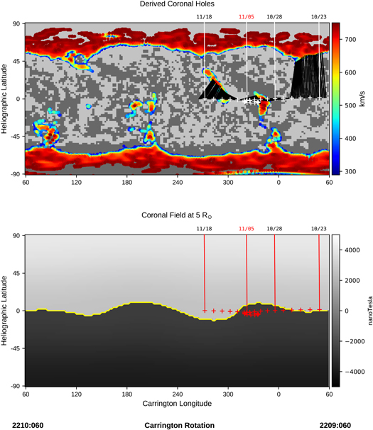
Figure 2. WSA-derived global coronal field, solar wind speed, and spacecraft magnetic connectivity to 1 R⊙ during the first solar encounter of the Parker Solar Probe. The last GONG observations assimilated into the ADAPT input map were from 2018 May 11 00:00:00 UTC at approximately 229° longitude. (Top) Derived coronal holes at 1 R⊙ with model-derived solar wind speed in colorscale. The field polarity at the photosphere is indicated by the light/dark (positive/negative) gray contours. White tick marks represent PSP's location mapped back to 5 R⊙ with dates labeled above in black, and the perihelion date (2018 May 11) in red. Black lines show connectivity between spacecraft and solar wind source region at 1 R⊙. (Bottom) Derived global coronal field (nT) at 5 R⊙. Red tick marks shown at a daily cadence represent PSP's location mapped back to 5 R⊙ with dates labeled above in black, and the perihelion date (2018 May 11) in red.
Download figure:
Standard image High-resolution imageOnce PSP was mapped back to the outer coronal boundary (i.e., 5 R⊙) of the model, the minimum angular distance between the spacecraft and the HCS was calculated. The result is depicted in Figure 3 (middle) as the red dots. This curve only appears to be piece-wise continuous due to the dynamic updates of the underlying photospheric maps. The jumps serve as a good measure of the uncertainty of the predictions. There is a good qualitative agreement between the predictions of this model and the PSP observations in Figure 3 (top). Small time deviations in the inbound leg are due to the low inclination of the HCS and the 2° quantization of the model. The several day disagreement early in November is likely due to the November 11–12 CME that is not included in the WSA model solution and has likely distorted the HCS.

Figure 3. Comparison of HCS crossings observed by PSP (top) and predicted by PFSS (middle) and MHD (bottom) models. The WSA PFSS model predictions are depicted with red dots, that of the 1.2  Badman model by blue ones, and that of the 2.0 R⊙ Badman model by green ones. The results from the Pogorelov MHD code are shown with a green line and that of Odstrcil ENLIL with red. See the text for more details.
Download figure:
Standard image High-resolution imageThe second PFSS-based model that we compared the PSP observation to explores a lower source surface radius and is from Badman et al. (2020) and Bale et al. (2019). The Badman model uses the open source pfsspy code (Yeates 2018; Stansby 2019) with a GONG magnetogram on 2018 November 6 to compute the magnetic fields at 1.2 R⊙ (and for comparison with the WSA model at 2.0 R⊙). The model then uses a ballistic propagation model (Nolte & Roelof 1973) to connect the PSP longitude with the source surface using measured radial velocity at PSP to generate a Parker spiral field line. The model assumes that the longitudinal velocity structure measured by PSP is latitudinally invariant and that the HCS does not evolve in shape between the source surface and PSP. While deviations from models that include current sheet modeling are expected, the polarity of the magnetic field should be preserved. The predicted angular distance of PSP from the HCS by the Badman PFSS model is shown in the middle panel of Figure 3 with a blue line for a 1.2 R⊙ source surface radius and with a green line for a 2.0 R⊙ source surface radius. The Badman PFSS model predicts the HCS further away from PSP than the WSA model. Using the lower, 1.2 R⊙ source surface radius, a more warped and inclined HCS is predicted that brings this model into closer agreement with the observations than the 2.0 R⊙ version, including predicting more polarity inversions in the inbound time interval (October 18 and 29). For the outbound leg, both PFSS models have very similar predictions although the 2.0 R⊙ model is more consistent with the timing of the outbound November 23 HCS crossing.
3.2. MHD Model Predictions
Besides PFSS models, we have compared the PSP observations of the HCS crossings with the predictions of magnetohydrodynamic (MHD) models. The PFSS-based models mentioned in the previous section combine the features of coronal and inner-heliospheric models and their results, as well as the results of any other coronal model, obtained above the critical surface can serve as boundary conditions for MHD models. The models described below use such boundary conditions, although they differ from each other. These differences are due to the physical processes taken into account in the coronal models, their implementation, and photospheric magnetograms used to run such models.
The Huntsville MHD model of the inner heliosphere (Borovikov et al. 2012; Kim et al. 2014, 2016; Pogorelov et al. 2017) is data-driven and designed to accept the inner boundary conditions beyond the critical surface from any coronal model. The model was implemented in the Multi-Scale Fluid-Kinetic Simulation Suite (MS-FLUKSS)—a suite of adaptive mesh refinement (AMR) codes (see Pogorelov et al. 2014, and references therein) built upon the Chombo AMR framework. This model tracks the position of the HCS surface from the inner boundary outwards using the level-set method (Borovikov et al. 2011). To run this model we use results from the WSA coronal model, which is described in the previous section, at the heliocentric distance of 21.5 R⊙. While the WSA model considers various sources of input at the solar surface, such as synoptic NSO/GONG magnetograms and the ADAPT model that provides a time sequence of synchronic maps by assimilating GONG or SDO/HMI LOS magnetograms into a flux-transport model using localized ensemble Kalmann filtering techniques (see, e.g., Hickmann et al. 2015). For this simulation, we use one particular realization (out of 12) of HMI-ADAPT-WSA maps that provides the best agreement with near-Earth solar wind data for the given period. The full simulation results for the first two complete PSP orbits are presented in detail by Kim et al. (2020) in this volume.
The magnetic sector polarity predictions of this MHD model is depicted in Figure 3 in the bottom panel with a green line. Here, the polarity is set to +1 or −1, where the level-set variable, which is used to track the HCS, acquires these values. The magnetic polarity is set to 0 in the region of numerical uncertainty surrounding the HCS, where the absolute value of the level-set variable is a fraction of unity.
There is a good qualitative agreement with the PSP observations except during the second half of the inbound leg of the PSP orbit. While PSP observations indicate primarily negative polarity between October 20 and 28, MS-FLUKSS predicts PSP to be traversing the region of numerical uncertainty along the HCS throughout this period. This indicates a low inclination HCS near the position of PSP. Just as in the case of the WSA PFSS model, PSP is likely to have flown closer to the HCS than the grid discretization in the MHD model allows. It is also understood that the results may be different either if the source surface position is changed or if another set of magnetograms is used.
Next we consider ENLIL, which is a 3D numerical model that uses ideal MHD description with a volumetric heating to simulate corotating and transient disturbances in the inner and mid heliosphere (Odstrcil 2003; Odstrcil et al. 2005). This model is observationally driven and can routinely predict heliospheric space weather, event-by-event, much faster than real time. Its operational version is used daily by forecasters at the NOAA/Space Weather Prediction Center and at the NASA/Community Coordinated Modeling Center. In this paper, a sequence of 90 WSA maps (derived from 1 hour cadence GONGz maps) at 21.5 Rs is used to calculate conditions for evolving background solar wind. Note that ENLIL computes the heliospheric magnetic field using a monopolar technique with solving an additional equation for tracing the polarity. This approach avoids artifacts associated with magnetic reconnections at HCSs and enables fast predictions on a grid with 2deg angular spacing and reliably identify the simulated HCS. The ENLIL results are shown also in Figure 3 in the bottom panel with a red line. The actual predicted crossing times are marked with a red dot and the uncertainty region around it with zero polarity. The predicted HCS crossing times are in good agreement with the PSP observations except on 2018 November 5. Though as the short zero polarity (within the uncertainty of the model to cross the HCS) region on 2018 October 28 suggests, the ENLIL predicted HCS surface is very close to the location of PSP, within the 2° grid size of the model.
Finally, we consider the predictions by Predictive Sciences Inc. (PSI) made months before the first PSP solar encounter. The PSI model uses the MAS code, which solves the set of resistive MHD equations in spherical coordinates on a nonuniform mesh. The details of the model have been described elsewhere (e.g., Mikič & Linker 1994; Lionello et al. 2001; Riley et al. 2001, 2011; Caplan et al. 2017; Mikič et al. 2018). The model is driven by the observed photospheric magnetic field, and for this study, HMI magnetograph observations from the SDO spacecraft were used to construct a boundary condition for the radial magnetic field at 1 R⊙ as a function of latitude and longitude. Since this was a prediction (i.e., made prior to PSP's first encounter), the map used was based on observations during Carrington rotation (CR) 2208 and 2209 (2018 September 2 to October 26, a solar rotation before the PSP closest approach). For computational efficiency, the model was run in two stages: first the region from 1 to 30 R⊙ is modeled, followed by the region from 30 R⊙ to 1 au, being driven directly by the results of the coronal calculation; however, we verified that the transition is seamless (Lionello et al. 2013). Additionally, this version of the model implements a wave-turbulence-driven approach for self-consistently heating the corona and invokes the WKB approximation for wave pressures, providing the necessary acceleration of the solar wind (Mikič et al. 2018). Further details of the model and prediction are provided by Riley et al. (2019). The PSI model predicted HCS crossing on October 21, 21:00 UT and on October 28, 21:00 UT, and a prolonged negative polarity during the closest approach time, consistent with PSP observations. A further two crossings were also predicted on November 19, 07:00 UT and on November 22, 20:00 UT. The predicted outbound crossing times differed from the observations, though it should be emphasized that this model predicted the HCS crossings using solar maps from a full solar rotation before the PSP encounter, and the outbound crossings were furthest in time from the input boundary conditions.
3.3. HCS Geometry
While there are notable differences between the various model results, a consensus result emerges for the global shape of the HCS during the first perihelion pass of PSP. It is generally agreed that during the inbound pass of the spacecraft, roughly between 2018 October 15 and November 4, the HCS had a very small inclination and PSP was traveling very close to it. Thus, the plasma sampled can be considered streamer belt material. On the other hand, outbound from the Sun, between 2018 November 15 and 23, the spacecraft travels further away from the HCS and it likely sampled solar wind emanating from a low latitude coronal hole.
4. 1 au Observations
Once we have established the global or large-scale geometry of the HCS at the location of PSP, we turn our attention to the evolution of the HCS from PSP's location to 1 au. It is expected that the geometry of the HCS would evolve as it propagates outward from the Sun impacted by the structured solar wind around it. Comparing PSP observations to 1 au measurements allows us to quantify this evolution.
To carry out this comparison, we have selected the Wind spacecraft orbiting the Sun–Earth first Lagrange point, near 1 au (STEREO observations were not available at the writing of this paper). The Wind spacecraft carries comparable instrumentation to enable this task. The magnetic field data is provided by the MFI instrument (Lepping et al. 1995), the solar wind proton measurement by the SWE Faraday Cup (Ogilvie et al. 1995), and the suprathermal electron observations by the 3DP instrument (Lin et al. 1995). Since PSP and Wind are not radially lined up (except on 2018 October 24), we have shifted the PSP measurements to the Sun–Earth longitude using the equatorial rotation rate of the Sun. While shifting backwards in time the PSP data minimizes the amount of transformation for the inbound leg of PSP's orbit, shifting forward requires less transformation for the outbound leg. To avoid artificial discontinuities, we have transformed the whole PSP data set both backward (Figure 4) and forward (Figure 5) in time. Since PSP reached super-corotation with the Sun at its closest approach, observing the same solar longitudes three times in a few days, the transformation to the Sun–Earth line is multivalued. This is evident around 2018 November 2 in Figure 4 and around 2018 November 28 in Figure 5. Fortunately, PSP was in a single negative sector during all of this time allowing a straightforward comparison with the Wind observations. This retrograde PSP orbit is also the reason we chose to transform the PSP measurements to the Wind solar longitude rather than vice versa.
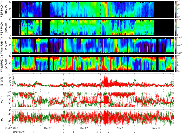
Figure 4. Comparison of HCS crossings observed by PSP and Wind with the PSP data backward shifted in time and the magnetic field scaled to 1 au. The upper two panels are the PSP 315 eV electron PADs (in flux units and normalized) propagated to the location of Wind. The next two panels are the 265 eV Wind electron PADs. The bottom three panels show the Wind observed magnetic field (green) and scaled PSP measurements (red) in spherical coordinates. Vertical dotted lines show the time of the propagated PSP HCS events identified by their region number from Table 1.
Download figure:
Standard image High-resolution image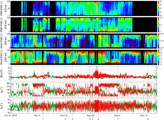
Figure 5. Comparison of HCS crossings observed by PSP and Wind with the PSP data forward shifted and magnetic field scaled. The upper two panels are the PSP 315 eV electron PADs (in flux units and normalized) propagated to the location of Wind. The next two panels are the 265 eV Wind electron PADs. The bottom three panels show the Wind observed magnetic field (green) and scaled PSP measurements (red) in spherical coordinates. Vertical dotted lines show the time of the propagated PSP HCS events identified by their region number from Table 1.
Download figure:
Standard image High-resolution imageNext the variable radial distance of PSP had to be taken into account. The observed PSP radial solar wind speed (that slowly increased from 300 to 500 km s−1 through the encounter) was used to propagate each time parcel to 1 au. This left the ±3° latitude of PSP relative to the ecliptic unaccounted for. We would have to do this individually for each crossing as this shift depends on the relative motion of the current sheet, whether it is moving northward or southward relative to Earth. In this study, we do not perform this transformation. For a current sheet tilted 30° with respect to the ecliptic a latitude difference of 3° results in a time shift of less than ± half day, which is small on the scale of the full encounter.
In order to allow comparison of the magnetic field measurements, the PSP measurements were also scaled. The radial component of the magnetic field is scaled by 1/r2 and the other two components by 1/r. While this is a somewhat simplistic scaling, it allows plotting the PSP and Wind data on the same scale for qualitative comparison.
Figures 4 and 5 show the transformed PSP data along with the corresponding Wind observations. The electron PAD measurements are stacked, while the magnetic field data is overplotted in the same panels with green for PSP and red for the transformed PSP observations. The eight PSP HCS crossing times are marked with vertical dashed lines. A remarkable amount of agreement can be found between the PSP and Wind observations. Not surprisingly, the larger inclination PSP HCS crossings on October 10 (PSP time, Event ID#1), on November 13–14 (#6), and on November 23 (#7) have very clear Wind equivalents. While the other HCS crossings are of a very low inclination current sheet, as discussed above, where small local corrugation of the surface or minute evolution of the shape can drastically change the timing of each encounter. The details of the Wind HCS crossings are tabulated in Table 2. To mark the connection between the Wind and PSP measurements in this table, the backward propagated PSP events are marked with an additional "a" label and the forward propagated ones with a "b." In spite of the somewhat tenuous correspondence between the low inclination, PSP and Wind HCS crossings this comparison confirms our previous result for the global geometry of the HCS. Namely, that during the PSP solar encounter the HCS was nearly parallel with the ecliptic but had a higher inclination while PSP was traveling away from the Sun.
Table 2. HCS Crossings Observed by Wind Corresponding to PSP Observations
| PSP Region | UT Start | time | Duration | Polarityb | Event Typec |
|---|---|---|---|---|---|
| ID#a | (YYYY-mm-dd) | (hh:mm:ss) | (hh:mm:ss) | ||
| PSP Inbound Events | |||||
| 1a | 2018 Oct 13 | 02:20:25 | 08:39:15 | +/+ | FR |
| 1a | 2018 Oct 13 | 11:24:55 | 05:33:48 | +/+ | FR |
| 1a | 2018 Oct 13 | 17:01:37 | 00:09:12 | +/− | HCS |
| 1b | 2018 Nov 8 | 14:24:00 | 21:10:16 | +/− | FR |
| 2a | 2018 Oct 19 | 21:29:55 | 33:57:15 | −/+ | BPe |
| 2a | 2018 Oct 21 | 07:23:10 | 04:24:03 | +/+ | HDR |
| 2b | 2018 Nov 18 | 11:15:07 | 08:56:54 | −/+ | FR |
| 2b | 2018 Nov 18 | 20:47: 13 | 17:58:15 | +/+ | LCSs |
| 3a | 2018 Oct 23 | 12:23:40 | 09:23:42 | +/− | eStrD, HDR? |
| 3b | 2018 Nov 19 | 14:45:28 | 07:43:00 | +/+ | FR |
| 3b | 2018 Nov 19 | 22:28:28 | 04:55:09 | +/− | HDR |
| 3b | 2018 Nov 20 | 01:38:04 | 00:02:45 | +/− | HCS, MFD |
| 4a | 2018 Oct 31 | 08:27:25 | 03:28:18 | −/− | FR |
| 4a | 2018 Oct 31 | 11:55:43 | 00:16:45 | −/+ | HCS, MFD |
| 4b,5b | 2018 Nov 24 | 02:35:46 | 23:36:25 | −/+/− | FR, HDR? |
| 5a | 2018 Nov 1 | 01:04:28 | 00:16:33 | +/− | HCS, MFD |
| 5a | 2018 Nov 1 | 1:21:01 | 03:25:12 | −/− | eStrD |
| PSP Outbound Events | |||||
| 6a | 2018 Nov 4 | 02:50:19 | 03:39:57 | −/− | eStrD |
| 6a | 2018 Nov 4 | 02:50:19 | 07:57:30 | −/+ | HDR |
| 6b | 2018 Dec 1 | 10:25:01 | 01:03:09 | −/+ | FR |
| 7a | 2018 Nov 8 | 14:24:00 | 21:10:16 | +/− | FR |
| 7b | 2018 Dec 6 | 17:57:01 | 00:30:57 | +/+ | FR, BPe |
| 7b | 2018 Dec 6 | 18:27:58 | 19:20:18 | +/− | HDR |
| 7b | 2018 Dec 6 | 20:16:13 | 00:18:33 | +/+ | FR, BPe |
| 7b | 2018 Dec 7 | 01:20:07 | 00:25:12 | +/− | HCS, MFD |
Notes.
aEvents with an "a" (ahead) suffix refers to PSP events propagated backwards in time to Wind's longitude; a suffix "b" (behind) refers to events propagated forward in time. As in Table 1, multiple substructures are associated with a single HCS crossing region. bMagnetic polarity of the region before and after the event. cCharacteristics of the event: HCS—single rapid crossing of current sheet, LCS—local current sheet, eStrD—electron strahl dropout, STR—stream with increased flow speed, MFD—magnetic field depression, HDR—high density region, FR—flux rope, BPe—bipolar electron heat flux, VMF—variable magnetic field.Download table as: ASCIITypeset image
5. The Structure of the HCS
Once we have established the global geometry of the HCS during the first PSP solar encounter, we turn our attention to the smaller solar wind structures in the immediate vicinity of the PSP magnetic sector crossings. Just as in the case of 1 au observations (Szabo et al. 1999a, 1999b; Sanchez-Diaz et al. 2019), it is rare to find a pristine, single sharp discontinuity marking the HCS in the PSP measurements. The various solar wind structures identified near magnetic polarity reversals in the PSP data are tabulated in the last column of Table 1. Single discontinuities with large magnetic field rotations concurrent with 180° changes in suprathermal electron PADs (marked as HCS in Table 1) were identified almost exclusively on the outbound leg where the HCS has a larger inclination. The most common feature during the inbound leg is a short duration (few hours) depression in the magnetic field magnitude (identified as MFD—magnetic field depression) concurrent with a pronounced increase in the radial speed of the solar wind (STR—stream) and electron strahl dropout (eStrD) sometimes also associated with elevated proton number density. An example of three such structures on 2018 October 9 and 10, near the HCS are shown in Figure 6. As will be discussed later, these structures do not have obvious counterparts in the Wind measurements (see the last column of Table 2). And we postulate that these disconnected and fast moving plasma parcels could evolve into the prominent high density regions (HDR), identified by Sanchez-Diaz et al. (2019) at 1 au, as they propagate outward and run into slower moving solar wind. HDRs are less prominent and frequent in the PSP observations compared to 1 au measurements. PSP observed a few small flux rope (FR) structures with a clear sense of slow rotation in the magnetic field, and some with bidirectional suprathermal electrons (BDe), though much smaller (3–10 hr) and more irregular than interplanetary coronal mass ejections. We have also identified a number of magnetic reconnection jets (Rec). They are usually found at discontinuities with large field rotation angles. Finally, we have identified three of the outbound HCS regions as variable magnetic field (VMF) periods where the magnetic field direction was disturbed for a significant period of time and none of the large field rotations were lined up with the electron PAD changes. These irregular structures along with signatures of magnetic reconnection indicate that inside the orbit of Venus the stream belt solar wind is still actively evolving.

Figure 6. PSP observations near the HCS crossing of 2018 October 9–10. The top two panels are the regular and normalized electron PAD, followed by the magnetic field in spherical coordinates. Finally, the bottom three panels show the proton radial speed, number density, and thermal speed. Three small disconnected streams are marked by vertical lines along with the magnetic polarity of each region.
Download figure:
Standard image High-resolution image
Since we have already connected the PSP HCS observations to 1 au Wind measurements of the current sheet (see Section 4 and Table 2), we can also compare the small solar wind structures associated with HCS at 1 au to the PSP observations. Unlike the large-scale geometry of the HCS, we do not expect to find one-to-one correlation between the small structures observed by PSP and Wind. However, we can look for general trends. Our results, based on Wind measurements, are consistent with the findings of Sanchez-Diaz et al. (2019) where they have identified sequences of sharp current sheet crossings (HCS), HDR, and small flux ropes (FR) interpreted as the in situ counterparts of streamer blobs observed in white light coronagraphs. The corresponding Wind observations have large flux ropes (FR), multihour long density enhancements (HDR), regions of bidirectional suprathermal electron (BPe) and strahl dropout (eStrD) times (see Table 2). However, as discussed above, PSP generally observed much smaller and qualitatively different structures (like the disconnected streams with magnetic field depressions). Based on these results, we conclude that the 1 au structures associated with the HCS are not direct remnants of similar coronal structures but are the end result of significant evolution in the inner heliosphere, changing the character of these structures.
6. Summary
In this paper, we have identified the HCS crossings of PSP during its first solar encounter. We have compared these HCS crossing times to the predictions of various heliospheric models and found a remarkable agreement. This gave us the confidence to conclude that the consensus global HCS geometry predicted by the models is correct. Namely that the HCS had a very low inclination relative to the solar rotational equator during the inbound leg of the PSP encounter keeping PSP very near it, while during the outbound leg the HCS moved further away. Thus, during the inbound leg, PSP observed uninterrupted streamer belt solar wind, while on the way away from the Sun PSP probably measured plasma from low latitude coronal holes.
We have also successfully related the PSP HCS observations to Wind measurements near Earth at 1 au. While we had to account for a variable and large correction due to the changing relative solar longitudes and radial distances of the two spacecraft, the PSP observed HCS crossings were successfully connected to 1 au observations. Thus, we have demonstrated that the global geometry of the HCS is relatively stable from near the Sun to 1 au and over a large portion of a solar rotation.
Finally, we have investigated small solar wind structures associated with the HCS and found significant differences between the PSP and Wind observations. We conclude that these small structures (often referred to as meso-scale structures) evolve significantly as they travel from the corona to 1 au, changing their size and even fundamental properties.
Parker Solar Probe was designed, built, and is now operated by the Johns Hopkins Applied Physics Laboratory as part of NASA's Living with a Star (LWS) program (contract NNN06AA01C). Support from the LWS management and technical team has played a critical role in the success of the Parker Solar Probe mission.
S.D.B. acknowledges the support of the Leverhulme Trust Visiting Professorship program. This work utilizes data produced collaboratively between Air Force Research Laboratory (AFRL) and the National Solar Observatory. The ADAPT model development is supported by AFRL.