


ABSTRACT
The outer edge of Saturn's B ring is strongly affected by the nearby 2:1 inner Lindblad resonance of Mimas and is distorted approximately into a centered elliptical shape, which at the time of the Voyager 1 and 2 encounters was oriented with its periapse toward Mimas. Subsequent observations have shown that the actual situation is considerably more complex. We present a complete set of historical occultation measurements of the B-ring edge, including the 1980 Voyager 1 and 1981 Voyager 2 radio and stellar occultations, the 1989 occultation of 28 Sgr, two independently analyzed occultations observed with the Hubble Space Telescope in 1991 and 1995, and a series of ring profiles from 12 diametric (ansa-to-ansa) occultations observed in 2005, using the Cassini Radio Science Subsystem (RSS). After making an approximate correction for systematic errors in the reconstructed spacecraft trajectories, we obtain orbit fits to features in the rings with rms residuals well under 1 km, in most cases. Fits to the B-ring edge in the RSS data reveal a systematic variation in the maximum optical depth at the very edge of the ring as a function of its orbital radius. We compare the B-ring measurements to an m = 2 distortion aligned with Mimas, and show that there have been substantial phase shifts over the past 25 years. Finally, we present freely precessing equatorial elliptical models for 16 features in the Cassini Division. The inner edges of the gaps are generally eccentric, whereas the outer edges are nearly circular, with ae < 0.5 km.
Export citation and abstract BibTeX RIS
1. INTRODUCTION
The sharp outer edge of B ring is one of the most prominent features in Saturn's ring system, forming the boundary between the optically thick and massive B ring itself and the more tenuous 4500 km wide Cassini Division. It has long been known that the B-ring edge lies near to the Mimas 2:1 Lindblad resonance (Smith et al. 1982), and from Voyager observations it became clear that the edge is quite non-circular, with radial excursions on the order of ±75 km. Porco et al. (1984) developed an appealing dynamical explanation for apparent m = 2 distortion of the B ring's shape as the result of a resonant interaction with Mimas. This model was supported by measurements of the variation in the radius of the edge from both Voyager 1 and 2 occultations and images of the ring, which showed that the periapse of the B-ring edge was closely aligned with Mimas. More recent observations have shown that the situation is considerably more complex. Bosh (1994) found that Hubble Space Telescope (HST) occultation measurements from 1991 ruled out the notion that the periapse was permanently aligned with Mimas, and Spitale et al. (2006) concluded from Cassini images that the m = 2 shape is misaligned with Mimas and that an additional m = 3 might be present as well. There is also the suggestion that the B-ring edge is chaotic (Spitale & Porco 2009). Using Cassini stellar occultation data, Hedman et al. (2009) and Nicholson et al. (2009) provided compelling evidence that the pattern speed of the B-ring edge differs from Mimas's mean motion, and proposed the provocative suggestion that the structure of the gaps and ringlets in the Cassini Division has a dynamical origin in the B ring itself (Hedman et al. 2010).
Any explanation for the time variability of the shape of the B ring must be consistent with the complete observational record. Here, we present precise, geometrically consistent occultation measurements of the B-ring edge from Voyager 1 (1980) and Voyager 2 (1981), from the widely observed occultation of 28 Sgr in 1989, from HST observations in 1991 and 1995, and from Cassini Radio Science Subsystem (RSS) observations of a series of diametric (ansa-to-ansa) ring occultations in 2005. These events span 25 years, and provide an important time history of the B ring prior to the onset of dense coverage of the B-ring shape from Cassini stellar occultation and imaging observations. In a companion paper, Hedman et al. (2010) make use of these measurements, as well as Cassini VIMS stellar occultation data, to develop time-variable models for the shape of the B-ring edge. Our results will eventually be useful for constraining the precession rate of Saturn's pole. Using the RSS data, we derive orbit fits to 16 sharp-edged features in the Cassini Division. Many of the inner edges of the gaps have measurable eccentricities, while their outer edges are very nearly circular, as also found by Hedman et al. (2009, 2010) and Nicholson et al. (2009).
In the following section, we describe the geometry of Saturn's ring system assumed for our analysis. Next, we present a new technique for determining the locations of sharp-edged ring features. We review the occultation observations in Section 4, and then present our summary of B-ring measurements in Section 5. Orbit fits to the Cassini Division features are given in Section 6, and we present our conclusions in the final section.
2. SATURN SYSTEM AND OCCULTATION GEOMETRY
The first highly accurate determination of the direction of Saturn's pole was obtained by Simpson et al. (1983) from Voyager Ultraviolet Spectrometer (UVS) and radio occultations. Nicholson et al. (1990) revisited and extended this work, using a more complete set of Voyager 1 and Voyager 2 occultation observations. The 1989 July 3 occultation of 28 Sgr provided important additional constraints on the pole direction: Hubbard et al. (1993) presented solutions based on the 28 Sgr data alone, while French et al. (1993, henceforth F93) included the Voyager occultation data as well, and demonstrated that Saturn's pole was precessing with a period of order 106 years. Elliot et al. (1993, henceforth E93) reported on the 1991 occultation of GSC 6323-01396 observed with the HST's High Speed Photometer (HSP), and derived a Saturn pole direction from the combination of 28 Sgr and HST measurements, but excluding the Voyager data. Bosh (1994) extended this analysis to include Voyager observations, largely confirming the F93 results and strengthening the detection of precession.
Ultimately, the incorporation of literally thousands of Cassini stellar and radio occultation measurements of individual ring features into a global solution for Saturn's pole direction and ring plane radius scale will substantially improve the measurement of the polar precession rate, which in turn will provide an important constraint on Saturn's moment of inertia and internal structure. To obtain the highest possible accuracy, this effort will require correction of small systematic errors in the Cassini spacecraft's reconstructed trajectory, however, which is well beyond the scope of the present effort. Here, we adopt the Saturn pole direction and precession rate given in Table 1, obtained from cpck11Jun2009.tpc, a recent planetary constants file provided by the Cassini Navigation Team.4 With this geometric constraint, we used the heliocentric vector algorithm described in Appendix A of F93 to determine the best-fitting sky-plane offsets f0 and g0 (compared to Equation (A15) of F93) for Earth-based occultations, timing offsets for selected observatories, along-track trajectory timing corrections for Voyager 1 and Voyager 2, and radii of the rings. We included measurements of nominally circular features, as identified in Table II of F93, except for features 1, 12, and 20, since these have subsequently proved to be measurably non-circular. With this exception, ring measurement times 28 Sgr and for Voyager 1 and Voyager 2 were identical to those used by F93 for their adopted geometry solution (their Table X). Measurements from the HST and Cassini RSS observations are described below.
Table 1. Saturn System Parameters and Adopted Occultation Geometry
| Parameter | Parameter or Value | Parameter or Value | Reference |
|---|---|---|---|
| Saturn pole (J2000) | α = 40 582542 582542 |
dα/dt = −0037432cy−1 |
|
| Epoch: 2000 Jan 1, 12:00:00 UTC | δ = 83537652 |
dδ/dt = −0004944cy−1 |
|
| J2 = 0.01629076 | RS = 60,330 km | Saturn GM = 3793120.721 km3 s−2 | |
| J4 = −0.00093517 | J6 = 0.00008954 | ||
| Adopted stellar coordinates (J2000) | α (h m s) | δ (d m s) | |
| Voyager 2 δ Sco | 16 00 20.0220 | −22 37 17.4936 | R. Jacobson (2009, private communication) |
| 28 Sgr | 18 46 20.58417 | −22 23 31.87202 | R. Jacobson (2009, private communication) |
| HST 1081 GSC 6323-01396 | 20 10 30.36698 | −20 36 47.49012 | R. Jacobson (2009, private communication) |
| HST 5824 GSC 5249-01240 | 23 19 34.5985 | −6 47 10.4737 | Bosh et al. (2002) |
| Sky-plane offsets | f0 (km) | g0 (km) | |
| 28 Sgr | −0.880 ± 0.252 | −0.624 ± 0.264 | |
| HST 1081 | 302.428 ± 0.278 | −52.320 ± 0.447 | |
| HST 5824 | 88.943 ± 0.546 | 188.526 ± 0.080 | |
| Time offsets | Station | s | |
| 28 Sgr | ESO (1m) | −0.213 ± 0.014 | |
| ESO (2m) | −0.198 ± 0.016 | ||
| MMT | +0.088 ± 0.018 | ||
| CAT | +0.029 ± 0.017 | ||
| SPM | −0.026 ± 0.012 | ||
| KPNO (ingress) | +0.063 ± 0.018 | ||
| KPNO (egress) | +0.066 ± 0.022 | ||
| Voyager 1 | DSS-63 | +0.020 ± 0.004 | |
| Voyager 2 | PPS | −0.063 ± 0.026 | |
| JPL planetary constants file | cpck11Jun2009.tpc | ftp://naif.jpl.nasa.gov | |
| Solar system ephemerides | sat286.bsp | " | |
| Spacecraft trajectory files | |||
| Voyager 1 | vgr1.sat286.bsp | Jacobson (2003) | ftp://naif.jpl.nasa.gov |
| Voyager 2 | vgr2.sat286.bsp | Jacobson (2003) | " |
| HST 1081 | h1e01s02.dat, h1e02s02.dat | http://archive.stsci.edu/hst | |
| h1e03s02.dat, h1e04s02.dat | " | ||
| HST 5824 | pfbl0000r.orx | " | |
| Cassini | 050606R_SCPSE_05114_05132.bsp | ftp://naif.jpl.nasa.gov | |
| 050623R_SCPSE_05132_05150.bsp | " | ||
| 050708R_SCPSE_05150_05169.bsp | " | ||
| 050802R_SCPSE_05169 05186.bsp | " | ||
| 050825R_SCPSE_05186_05205.bsp | " | ||
| 050907R_SCPSE_05205_05225.bsp | " | ||
| 050922R_SCPSE_05225_05245.bsp | " | ||
| 051011R_SCPSE_05245_05257.bsp | " |
Download table as: ASCIITypeset image
Our orbit fitting code differs in several important respects from that used by F93. The new code, RINGFIT, is implemented in IDL, a commercial programming language available from ITT Visual Information Solutions. We make extensive use of the ICY interface to NASA's NAIF SPICE toolkit (Acton 1996), which provides easy access to planetary ephemerides and spacecraft trajectory files. We use the J2000 heliocentric reference frame, the IAU 1976 model for the Earth shape (Abalakin 1981), and the ITRF93 Earth rotation model (Boucher et al. 1994). We account for general relativistic deflection by Saturn (including the effect of J2) for Earth-based stellar occultations only, solving for the deflection at the time the occultation ray is closest to Saturn in the sky plane, rather than the time the occultation ray penetrates the ring plane, as implied by Equations (A20)–(A23) of F93 (this difference amounts to only a few meters in the derived ring plane radius). We also make use of Earth observatory positions as tabulated by JPL's Horizons (Giorgini et al. 1996). Our adopted Saturn system parameters, occultation star coordinates (corrected for parallax and proper motion for the circumstances of each occultation), planetary ephemerides, spacecraft trajectory files, and fit results are included in Table 1.
3. DETERMINATION OF RING FEATURE LOCATIONS
The fundamental observations used for determining the geometry of Saturn's ring system are the measured times in occultation light curves of recognizable edges of ringlets and gaps, and the midtimes of narrow features. For previous investigations of the rings of Saturn and Uranus, we modeled ring features as intrinsically sharp-edged, with smoothing due to diffraction, the finite angular diameter of the occulted star, and the instrumental response time (Elliot et al. 1984; French et al. 1993). This approach was adequate for the 1989 July 3 Saturn stellar occultation of 28 Sgr, with a projected stellar diameter of about 18 km, but is difficult to apply to high-resolution occultations of ring structure that often show intrinsically ragged or gradual variations in optical depth near the edges of recognizable features. In anticipation of the wealth of Cassini occultation measurements of more than a hundred distinct features in Saturn's rings, we have written an interactive IDL program, RINGMASTER, that incorporates all available Saturn ring occultation data, selectively overplots them in orbital radius, and enables the user to fit a variety of analytic models to ringlets and ring edges.
We begin by normalizing each occultation observation to form the intensity I(t) as a function of time, where I = 1 in the absence of ring opacity and I = 0 for a perfectly opaque ring. It is useful to convert I(t) to the inferred normal optical depth τ(r') from

where B is the opening angle of Saturn's equatorial plane and r' is the radius in the equatorial plane, computed from the observed time t using a provisional model of the occultation geometry for each occultation. (We denote the radius as r', rather than r, as a reminder that the actual radius of the feature r is yet to be determined from a global solution for the geometry of the entire ring system, including the possibility that the ring is inclined relative to Saturn's equator.) This approach allows for easy intercomparisons of radial profiles of ring structure from different observations. All of the least-squares fits for locations of ring features are performed as a function of r', and the corresponding geometry-independent event time t(r') is determined by interpolation.
For narrow ringlets, we adopt Gaussian, Lorentzian, or Voigt profiles. For broader features, we experimented with several representations of the ring edge to be fitted. Of the variety of ramp-like functions we tried, the logistic function gave the most reproducible results. Initially, we fitted the τ(r') profile for the radial location r'1/2 at which the optical depth of a gap or ringlet edge reached half its maximum value relative to the background optical depth in the immediate vicinity of both sides of the feature, using a logistic function to represent the model normal optical depth, τm:
where σ controls the gradualness of the ramp; the lower baseline has optical depth τ0 and the full optical depth of the edge feature is τ0 + τ1. The upper/lower signs apply to rising/falling edges in optical depth, respectively.
We found, however, that uncertainties in the derived optical depth of nearly opaque ring edges, and variations in edge shape for the same feature in different data sets and at different ring longitudes, resulted in rather large scatter in the fitted radii. As an alternative, we fitted a logistic model function to the normalized signal profile I(r') itself, using
where I0 is the fitted lower signal level, I1 is the amplitude of the edge feature in units of the normalized stellar intensity, and once again σ is a measure of the sharpness of the edge. The upper/lower signs are used for falling/rising edges (in intensity), respectively. This resulted in more stable results, but when comparing ring profiles from multiple data sets taken at a range of ring opening angles, the effects of the sin |B| foreshortening factor affected the shapes of the profiles.
In the end, we adopted the strategy of constructing a geometry-independent "pseudo-intensity profile" to represent the normalized intensity that would be measured when viewing the ring at normal incidence (sin |B| = 1):

To preserve the convention that increasing optical depth increases vertically on a plot, we flipped the curve vertically using the auxiliary function

and fit a logistic model function to an edge profile using
with the mid-point r'1/2 of the feature defined to be where  (Note that, in general, the mid-point determined from the pseudo-intensity
  will differ from that determined from the normalized signal profile I(r') because τ differs from τ/sin |B|.) We found this approach to be the most stable of the three, while preserving the desirable characteristic of being able to represent on a common footing multiple profiles observed at different ring opening angles.
4. OBSERVATIONS
For the present analysis of the B-ring edge, we make use of unpublished results obtained by F93 as part of their analysis of the Voyager and 28 Sgr occultations, as well as independent reanalyses of two HST occultations. We use recent Cassini RSS occultation measurements to complete our data set for the B-ring edge, and for measurements of gap edges in the Cassini Division. Here, we describe the observations and our ring measurements. We defer the collected tabulation of the B-ring measurements themselves and a detailed discussion of the B-ring shape to Section 5; we leave the orbit fits to the Cassini Division features for Section 6.
4.1. Voyager 1 and 2
The first high-resolution occultation measurements of Saturn's rings were obtained from the Voyager 1 RSS egress occultation of 1980 November 13, which scanned the entire ring region at wavelengths λ = 3.6 cm (X band) and λ = 13 cm (S band; Tyler et al. 1983). Using a Fresnel inversion technique to remove the effects of diffraction, Marouf et al. (1986) obtained sub-km resolution profiles of all but the most opaque parts of the rings, where low ring opening angle (B ≃ 6°) resulted in extinction of the received signal to below the noise floor. Then, during the Voyager 2 encounter of 1981 August 25/26, the egress occultation of δ Sco was observed with the Photopolarimeter (PPS; Lane et al. 1982; Esposito et al. 1983, 1987) and the UVS (Sandel et al. 1982; Holberg et al. 1982) ultraviolet instruments. Simpson et al. (1983) and Nicholson et al. (1990) used the joint Voyager 1 and 2 occultation measurements to determine Saturn's pole direction and radius scale. F93 made independent measurements of the occultation event times of ring features from the RSS, PPS, and UVS data sets as part of their determination of the Saturn system geometry. As part of their work, F93 measured (but did not publish) the times of discernible sharp-edged non-circular features, including the B-ring outer edge (designated Feature 55 in F93, Table II). For consistency with these previous results, we use the unpublished Voyager 1 and 2 B-ring outer edge ring times obtained by F93 for the RSS and PPS data sets, and determine the ring plane radius according to the orbit fit results given in Table 1 (see Section 5). Logistic model fits to the high-resolution Voyager RSS and PPS data agreed with the F93 B-ring edge measurements to within a small fraction of a second, corresponding to a few tenths of a km difference at most. The UVS occultation data have substantially lower time resolution than the PPS measurements of the same occultation, and we exclude them from this study.
4.2. 28 Sgr Occultation
The 1989 July 3 occultation of 28 Sgr remains the most widely observed Earth-based occultation to reveal the detailed structure of Saturn's rings. F93 and Hubbard et al. (1993) describe in detail their observations of the event from 11 telescopes in Hawaii and North and South America. For this study, we used the unpublished F93 B-ring edge times obtained from Palomar Observatory, McDonald Observatory, NASA's Infrared Telescope Facility (IRTF), and the European Southern Observatory (ESO) 1 and 2 m telescopes. These are high signal-to-noise detections, limited in resolution primarily by the rather large (∼18 km) projected diameter of the occulted star at Saturn's distance from the Earth. The F93 measurements are used in preference to logistic model fits both for self-consistency with previously published results, and because the conversion from observed intensity I(t) to the pseudo-intensity  used for our logistic model fits makes it somewhat complicated to account properly for the smoothing effects of the occulted star. We used the orbit fit documented in Table 1 to convert from ring event time to ring plane radius.
4.3. HST Observations
Three HST occultation observations of Saturn's rings were obtained during the interval between the 28 Sgr event and the commencement of intensive Cassini occultation observations in 2005. Two of these, described in more detail below, crossed the B-ring outer edge; a third event, the 1993 October 12 occultation of GSC 5800-00460 observed with the HST's HSP as part of HST program 3373 (Bless 1992), crossed only the C and inner B ring and is not included in this investigation.
4.3.1. HST Program 1081
The 1991 October 2/3 stellar occultation of GSC 6323-01396 by Saturn's rings was observed with the HSP as part of HST program 1081. This was an exceedingly slow event, resulting in multiple passages across many ring features due to the parallactic shift of the star relative to Saturn induced by the HST's rapid orbital motion around the Earth. E93 published an extensive analysis of this occultation, and used the results to derive a revised Saturn pole direction and ring radius scale. They also produced a catalog of ring features detected in the occultation light curves. To check these results, and for consistency with our other ring feature measurements, we performed a completely independent analysis of these observations. We obtained the pipeline-processed HST 1081 data and spacecraft ephemeris from the Space Telescope Science Institute's (STScI) online data archives. The retrieved data files post-date the E93 work, and the start times of the current online files from STScI differ by a few tenths of a second from those reported by E93. Table 2 lists the data sets used, and compares the start times of each segment with those given by E93. For nearly all segments, the new start times are earlier by dtseg = −0.381 s than those used by E93. The single exception is segment 5, for which there are no measurable ring features. We extracted individual segments of the occultation light curve, subtracted polynomial background levels, and estimated the full stellar intensity to produce normalized signal profiles I(t) from each file in a similar fashion to E93.
Table 2. HST 1081 Data Segment Start Times
| Obs. ID | Segment | tseg (UTC) | E93 tseg (UTC) | dtseg |
|---|---|---|---|---|
| v0rr6401 | 1 | 1991 Oct 02 19:35:10.2149 | 1991 Oct 2 19:35:10.5956 | −0.3807 |
| v0rr6402 | 2 | 1991 Oct 02 21:10:54.2148 | 1991 Oct 2 21:10:54.5955 | −0.3807 |
| v0rr6403 | 3 | 1991 Oct 02 21:35:49.2147 | 1991 Oct 2 21:35:49.5955 | −0.3808 |
| v0rr6404 | 4 | 1991 Oct 02 22:47:32.2146 | 1991 Oct 2 22:47:32.5957 | −0.3811 |
| v0rr6405 | 5 | 1991 Oct 02 23:24:35.1397 | 1991 Oct 2 23:24:35.5948 | −0.4551 |
| v0rr6406 | 6 | 1991 Oct 03 00:24:09.2148 | 1991 Oct 3 00:24:09.5956 | −0.3808 |
| v0rr6407 | 7 | 1991 Oct 03 02:00:47.2147 | 1991 Oct 3 02:00:47.5957 | −0.3810 |
| v0rr6408 | 8 | 1991 Oct 03 03:37:24.2149 | 1991 Oct 3 03:37:24.5949 | −0.3800 |
| v0rr6409 | 9 | 1991 Oct 03 05:14:01.2152 | 1991 Oct 3 05:14:01.5958 | −0.3806 |
| v0rr640a | 10 | 1991 Oct 03 06:50:39.2151 | 1991 Oct 3 06:50:39.5958 | −0.3807 |
| v0rr640b | 11 | 1991 Oct 03 08:27:16.2153 | 1991 Oct 3 08:27:16.5959 | −0.3806 |
| v0rr640c | 12 | 1991 Oct 03 10:03:54.2151 | 1991 Oct 3 10:03:54.5951 | −0.3800 |
| v0rr640d | 13 | 1991 Oct 03 11:40:30.2148 | 1991 Oct 3 11:40:30.5949 | −0.3801 |
| v0rr640e | 14 | 1991 Oct 03 13:17:08.2147 | 1991 Oct 3 13:17:08.5959 | −0.3812 |
| v0rr640f | 15 | 1991 Oct 03 14:53:46.2155 | 1991 Oct 3 14:53:46.5969 | −0.3814 |
Download table as: ASCIITypeset image
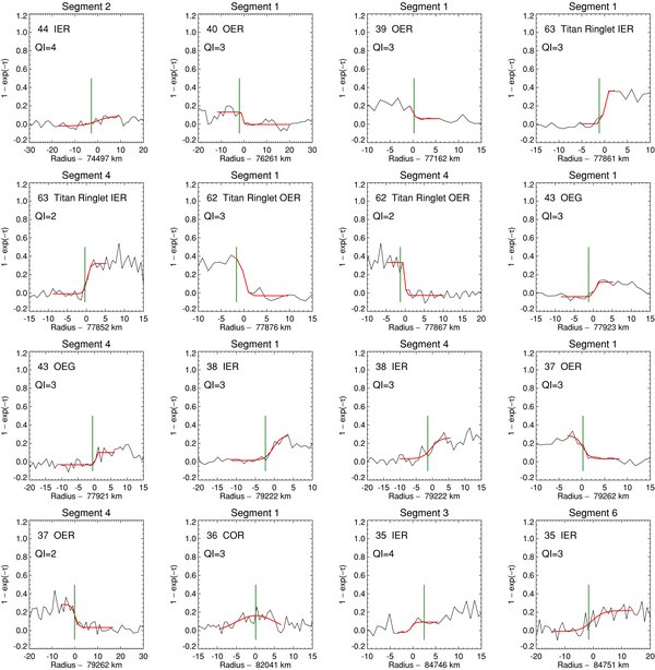
As described previously, we used RINGMASTER to determine the location of every clearly identifiable ring feature in the HST 1081 data set, as shown in Figure 1 and tabulated in Table 3. In each panel, we plot  at full resolution as a function of the true ring plane radius r derived from the orbit solution described in Section 2. The time resolution of the data is 0.15 s per point, although the corresponding radial resolution varies considerably because of the varying effect of the projected HST's orbital velocity on the radial component of the velocity of the occultation in Saturn's ring plane. The red curves show the logistic model fit,
  . Each panel is identified by the data segment containing the feature (see Table 3 of E93), the feature number from F93, and a feature label, using IE and OE to designate the inner and outer edges, respectively, of ringlets (R) and gaps (G). COR denotes the center of a ringlet.
Download figure:
Standard image High-resolution image
Download figure:
Standard image High-resolution image
Download figure:
Standard image High-resolution image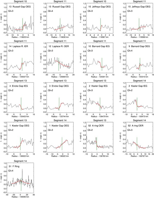
Figure 1. Gallery of ring features from the 1991 October 2/3 stellar occultation of GSC 6323-01396 observed from the HST under program 1081. Each panel is identified by observation segment number, ring feature number (following F93), and feature type (IE and OE for the inner and outer edge; G for gap and R for ringlet; COR for the center of ringlet). The quality index, QI, is a subjective measure of data quality, with 1 being the best and 4 corresponding to a questionable detection. Each profile is plotted as a function of derived ring plane radius, at full resolution (0.15 s per point) in terms of 1 − exp(−τ), where τ is the normal optical depth. The red curves correspond to the best-fitting logistic model. The green vertical lines mark the locations of features as measured by E93. In general, the agreement is satisfactory, although in some cases, we assign QI = 4 to features we regard as suspect. See Table 3 for details.
Download figure:
Standard image High-resolution imageWe also include a subjective quality index (QI), according to the following scale: QI = 1 represents a perfect, virtually noise-free fit; QI = 2 corresponds to good fit, with some noticeable deviation between model and observation; QI = 3 is for a fair fit, with substantial noise or deviation between shape of model and shape of feature (we also assign QI = 3 to otherwise high SNR observations with poor spatial resolution); and QI = 4 represents a barely detectable feature, with a significant chance that the putative ring feature is not actually present in the data. (Note that E93 assign a confidence level of 2 for a certain detection and 1 for a probable detection.) We assign QI = 3 to most of the features in this data set.
We made a detailed comparison of our fitted event locations with those given in Table 3 of E93, marked by a vertical green bar in each panel of Figure 1. In most cases, our fitted event locations agree quite well, although we reject as too noisy several features that they identified as certain detections (see, for example, segment 11 feature 18 in Figure 1 and segment 11 feature 13 in Figure 1), and in a few instances our measurements differ by several km from the E93 results. Because both the absolute times of our data files and our underlying geometrical solution for the rings differ from those used by E93, we have computed several auxiliary quantities to clarify the differences between our independent measurements of the ring features. In addition to the UTC time t0 of our measurements, we include in Table 3 the time of each feature measured relative to the start of the data file for the corresponding data segment, Δtseg. We also include the inferred corresponding quantity for the E93 analysis, computed from their tabulated ring event times and segment start times.
Table 3. HST 1081 Ring Events
| ID | Label | Seg. | Observed Time, t0 | QI | E93 | Δtsega | E93 Δtsegb | dtc | drd | r |  |
λ |
|---|---|---|---|---|---|---|---|---|---|---|---|---|
| (UTC) | Conf | (s) | (s) | (s) | (km) | (km) | (km s−1) | (°) | ||||
| 44 | IER 44 F93 | 2 | 1991 Oct 02 21:17:51.063 ± 0.287 | 4 | 2 | 416.848 | 416.505 | −0.343 | −2.508 | 74496.696 | 7.308 | 266.584 |
| 40 | OER 40 F93 | 1 | 1991 Oct 02 19:54:11.262 ± 0.110 | 3 | 2 | 1141.047 | 1140.874 | −0.172 | −1.524 | 76260.548 | 8.841 | 275.603 |
| 39 | OER 39 F93 | 1 | 1991 Oct 02 19:55:54.492 ± 0.100 | 3 | 2 | 1244.277 | 1244.284 | 0.008 | 0.067 | 77162.185 | 8.613 | 276.057 |
| 63 | Titan Ringlet IER | 1 | 1991 Oct 02 19:57:16.773 ± 0.044 | 3 | 2 | 1326.558 | 1326.424 | −0.133 | −1.114 | 77860.928 | 8.363 | 276.424 |
| 4 | 1991 Oct 02 22:48:31.229 ± 0.043 | 2 | 2 | 59.014 | 58.904 | −0.110 | −0.604 | 77852.227 | 5.515 | 260.617 | ||
| 62 | Titan Ringlet OER | 1 | 1991 Oct 02 19:57:18.577 ± 0.033 | 3 | 2 | 1328.362 | 1328.164 | −0.198 | −1.651 | 77876.011 | 8.356 | 276.432 |
| 4 | 1991 Oct 02 22:48:33.935 ± 0.050 | 2 | 2 | 61.720 | 61.454 | −0.266 | −1.470 | 77867.169 | 5.529 | 260.616 | ||
| 43 | OEG 43 F93 | 1 | 1991 Oct 02 19:57:24.256 ± 0.043 | 3 | 2 | 1334.041 | 1333.844 | −0.197 | −1.638 | 77923.408 | 8.337 | 276.458 |
| 4 | 1991 Oct 02 22:48:43.690 ± 0.100 | 3 | 2 | 71.475 | 71.304 | −0.171 | −0.953 | 77921.341 | 5.579 | 260.616 | ||
| 38 | IER 38 F93 | 1 | 1991 Oct 02 20:00:06.189 ± 0.063 | 3 | 2 | 1495.974 | 1495.704 | −0.270 | −2.066 | 79221.714 | 7.661 | 277.178 |
| 4 | 1991 Oct 02 22:52:17.575 ± 0.151 | 3 | 2 | 285.360 | 285.204 | −0.156 | −1.017 | 79221.583 | 6.539 | 260.775 | ||
| 37 | OER 37 F93 | 1 | 1991 Oct 02 20:00:11.487 ± 0.058 | 3 | 2 | 1501.272 | 1501.274 | 0.002 | 0.016 | 79262.235 | 7.636 | 277.201 |
| 4 | 1991 Oct 02 22:52:23.747 ± 0.076 | 2 | 2 | 291.533 | 291.504 | −0.028 | −0.186 | 79262.013 | 6.563 | 260.785 | ||
| 36 | COR 36 F93 | 1 | 1991 Oct 02 20:07:32.438 ± 0.176 | 3 | 2 | 1942.223 | 1942.214 | −0.009 | −0.040 | 82041.136 | 4.738 | 278.982 |
| 35 | IER 35 F93 | 3 | 1991 Oct 02 21:39:55.041 ± 0.055 | 4 | 2 | 245.826 | 246.305 | 0.478 | 2.830 | 84745.635 | 5.919 | 272.010 |
| 6 | 1991 Oct 03 00:27:21.516 ± 0.209 | 3 | 2 | 192.301 | 192.104 | −0.197 | −1.178 | 84750.575 | 5.988 | 255.907 | ||
| 34 | OER 34 F93 | 3 | 1991 Oct 02 21:40:30.053 ± 0.046 | 3 | 2 | 280.838 | 280.705 | −0.133 | −0.761 | 84949.055 | 5.701 | 272.161 |
| 6 | 1991 Oct 03 00:27:53.815 ± 0.100 | 3 | 2 | 224.600 | 224.654 | 0.054 | 0.332 | 84945.817 | 6.103 | 255.948 | ||
| 33 | IER 33 F93 | 3 | 1991 Oct 02 21:42:45.797 ± 0.303 | 3 | 2 | 416.582 | 416.455 | −0.127 | −0.610 | 85662.062 | 4.786 | 272.718 |
| 6 | 1991 Oct 03 00:29:47.547 ± 0.046 | 3 | 2 | 338.332 | 338.204 | −0.127 | −0.822 | 85660.883 | 6.462 | 256.145 | ||
| 42 | OER 42 F93 | 3 | 1991 Oct 02 21:43:07.100 ± 0.407 | 3 | 2 | 437.885 | 437.705 | −0.181 | −0.837 | 85762.387 | 4.633 | 272.801 |
| 31 | IER 31 F93 | 3 | 1991 Oct 02 21:43:42.275 ± 0.087 | 3 | 2 | 473.060 | 473.055 | −0.005 | −0.023 | 85920.804 | 4.374 | 272.935 |
| 6 | 1991 Oct 03 00:30:27.624 ± 0.200 | 4 | 2 | 378.409 | 378.204 | −0.204 | −1.343 | 85922.088 | 6.573 | 256.233 | ||
| 30 | IER 30 F93 | 3 | 1991 Oct 02 21:45:36.426 ± 0.280 | 3 | 2 | 587.211 | 587.305 | 0.093 | 0.327 | 86370.392 | 3.494 | 273.340 |
| 6 | 1991 Oct 03 00:31:35.233 ± 0.100 | 3 | 1 | 446.018 | 445.604 | −0.413 | −2.785 | 86372.205 | 6.740 | 256.403 | ||
| 29 | OER 29 F93 | 3 | 1991 Oct 02 21:46:49.135 ± 0.100 | 3 | 2 | 659.920 | 660.175 | 0.254 | 0.739 | 86603.034 | 2.903 | 273.574 |
| 6 | 1991 Oct 03 00:32:09.150 ± 0.100 | 3 | 2 | 479.936 | 479.704 | −0.231 | −1.575 | 86602.060 | 6.814 | 256.498 | ||
| 61 | Maxwell Ringlet IER | 6 | 1991 Oct 03 00:34:15.515 ± 0.058 | 3 | 2 | 606.300 | 606.104 | −0.196 | −1.377 | 87477.953 | 7.035 | 256.902 |
| 60 | Maxwell Ringlet OER | 6 | 1991 Oct 03 00:34:23.059 ± 0.101 | 3 | 2 | 613.844 | 613.904 | 0.060 | 0.422 | 87531.065 | 7.046 | 256.928 |
| 56 | 1.495 RS OER | 7 | 1991 Oct 03 02:01:03.956 ± 0.048 | 3 | 2 | 16.742 | 16.874 | 0.133 | 0.692 | 90202.833 | 5.214 | 251.752 |
| 24 | IER 24 F93 | 7 | 1991 Oct 03 02:01:42.534 ± 0.133 | 3 | 2 | 55.320 | 54.504 | −0.815 | −4.368 | 90406.730 | 5.357 | 251.766 |
| 23 | OER 23 F93 | 7 | 1991 Oct 03 02:02:21.112 ± 0.713 | 4 | 2 | 93.898 | 94.004 | 0.107 | 0.586 | 90615.991 | 5.492 | 251.789 |
| 82 | OEG 82 F93 | 7 | 1991 Oct 03 02:14:49.582 ± 0.155 | 3 | 2 | 842.367 | 842.204 | −0.163 | −1.090 | 95347.792 | 6.688 | 253.890 |
| 55 | B ring OER | 10 | 1991 Oct 03 07:14:26.700 ± 0.100 | 3 | 2 | 1427.484 | 1427.254 | −0.230 | −0.947 | 117509.045 | 4.113 | 247.650 |
| 11 | 1991 Oct 03 08:29:48.106 ± 0.154 | 3 | 2 | 151.891 | 151.654 | −0.237 | −1.187 | 117548.622 | 5.008 | 240.841 | ||
| 54 | Huygens Ringlet IER | 10 | 1991 Oct 03 07:15:41.215 ± 0.108 | 3 | 2 | 1502.000 | 1501.854 | −0.146 | −0.563 | 117805.761 | 3.849 | 247.978 |
| 11 | 1991 Oct 03 08:30:37.086 ± 0.274 | 3 | 2 | 200.871 | 201.004 | 0.133 | 0.675 | 117795.378 | 5.068 | 240.918 | ||
| 53 | Huygens Ringlet OER | 10 | 1991 Oct 03 07:15:45.513 ± 0.119 | 3 | 2 | 1506.298 | 1506.104 | −0.194 | −0.742 | 117822.265 | 3.833 | 247.997 |
| 11 | 1991 Oct 03 08:30:41.392 ± 0.154 | 3 | 2 | 205.177 | 204.904 | −0.273 | −1.385 | 117817.207 | 5.072 | 240.925 | ||
| 20 | Huygens Gap OEG | 10 | 1991 Oct 03 07:16:14.662 ± 0.108 | 4 | 2 | 1535.447 | 1535.254 | −0.193 | −0.719 | 117932.397 | 3.724 | 248.123 |
| 11 | 1991 Oct 03 08:31:03.899 ± 0.176 | 3 | 1 | 227.684 | 227.504 | −0.180 | −0.917 | 117931.627 | 5.096 | 240.965 | ||
| 19 | Herschel Gap IEG | 10 | 1991 Oct 03 07:17:28.053 ± 0.100 | 3 | 2 | 1608.838 | 1608.804 | −0.033 | −0.115 | 118195.152 | 3.435 | 248.435 |
| 11 | 1991 Oct 03 08:31:54.531 ± 0.100 | 3 | 2 | 278.316 | 278.204 | −0.112 | −0.574 | 118190.860 | 5.144 | 241.063 | ||
| 18 | R7 IER | 10 | 1991 Oct 03 07:17:39.331 ± 0.178 | 3 | 2 | 1620.116 | 1619.804 | −0.312 | −1.056 | 118233.621 | 3.389 | 248.482 |
| 11 | 1991 Oct 03 08:32:01.844 ± 0.400 | 4 | 2 | 285.629 | 285.404 | −0.224 | −1.156 | 118228.490 | 5.150 | 241.079 | ||
| 17 | R7 OER | 11 | 1991 Oct 03 08:32:08.262 ± 0.079 | 3 | 2 | 292.047 | 292.004 | −0.043 | −0.221 | 118261.554 | 5.155 | 241.092 |
| 16 | Herschel Gap OEG | 10 | 1991 Oct 03 07:17:54.277 ± 0.350 | 3 | 2 | 1635.062 | 1634.604 | −0.458 | −1.522 | 118283.794 | 3.327 | 248.543 |
| 11 | 1991 Oct 03 08:32:12.679 ± 0.156 | 3 | 2 | 296.464 | 296.404 | −0.060 | −0.309 | 118284.326 | 5.158 | 241.102 | ||
| 13 | Russell Gap OEG | 10 | 1991 Oct 03 07:19:46.203 ± 0.100 | 3 | 2 | 1746.988 | 1746.804 | −0.184 | −0.521 | 118629.129 | 2.839 | 248.991 |
| 11 | 1991 Oct 03 08:33:19.453 ± 0.396 | 4 | 2 | 363.238 | 363.204 | −0.034 | −0.174 | 118630.246 | 5.202 | 241.255 | ||
| 15 | Jeffreys Gap OEG | 10 | 1991 Oct 03 07:21:59.839 ± 0.100 | 3 | 2 | 1880.624 | 1880.504 | −0.119 | −0.263 | 118966.662 | 2.206 | 249.484 |
| 11 | 1991 Oct 03 08:34:24.242 ± 0.342 | 3 | 2 | 428.027 | 427.904 | −0.123 | −0.641 | 118968.160 | 5.229 | 241.422 | ||
| 14 | 1.990 RS IER | 11 | 1991 Oct 03 08:37:48.547 ± 0.100 | 3 | 2 | 632.332 | 632.504 | 0.173 | 0.900 | 120037.441 | 5.216 | 242.053 |
| 12 | 1.990 RS OER | 11 | 1991 Oct 03 08:37:54.591 ± 0.785 | 3 | 2 | 638.375 | 638.004 | −0.371 | −1.936 | 120068.953 | 5.213 | 242.074 |
| 10 | Barnard Gap IEG | 11 | 1991 Oct 03 08:38:39.250 ± 0.100 | 3 | 2 | 683.035 | 683.304 | 0.269 | 1.399 | 120301.236 | 5.190 | 242.232 |
| 9 | Barnard Gap OEG | 11 | 1991 Oct 03 08:38:41.859 ± 0.376 | 4 | 2 | 685.644 | 685.754 | 0.110 | 0.571 | 120314.775 | 5.188 | 242.241 |
| 4 | Encke Gap IEG | 13 | 1991 Oct 03 11:53:07.032 ± 0.017 | 2 | 2 | 756.817 | 756.845 | 0.028 | 0.129 | 133420.446 | 4.551 | 238.848 |
| 3 | Encke Gap OEG | 13 | 1991 Oct 03 11:54:18.906 ± 0.051 | 2 | 2 | 828.691 | 828.475 | −0.216 | −0.963 | 133744.277 | 4.459 | 239.110 |
| 2 | Keeler Gap IEG | 13 | 1991 Oct 03 12:06:46.577 ± 0.210 | 3 | 2 | 1576.363 | 1576.445 | 0.083 | 0.213 | 136478.993 | 2.581 | 242.074 |
| 14 | 1991 Oct 03 13:18:08.137 ± 0.050 | 2 | 2 | 59.922 | 60.034 | 0.112 | 0.501 | 136474.734 | 4.485 | 235.649 | ||
| 1 | Keeler Gap OEG | 13 | 1991 Oct 03 12:07:03.558 ± 0.086 | 2 | 2 | 1593.343 | 1593.255 | −0.088 | −0.221 | 136522.281 | 2.519 | 242.138 |
| 14 | 1991 Oct 03 13:18:18.586 ± 0.179 | 3 | 2 | 70.371 | 70.304 | −0.067 | −0.302 | 136521.637 | 4.494 | 235.660 | ||
| 52 | A ring OER | 13 | 1991 Oct 03 12:08:56.362 ± 0.080 | 2 | 2 | 1706.147 | 1706.125 | −0.022 | −0.047 | 136782.703 | 2.095 | 242.548 |
| 14 | 1991 Oct 03 13:19:12.865 ± 0.216 | 3 | 2 | 124.650 | 124.574 | −0.076 | −0.343 | 136766.552 | 4.531 | 235.727 | ||
| 51 | F Ring | 14 | 1991 Oct 03 13:31:37.012 ± 0.573 | 4 | 1 | 868.798 | 869.404 | 0.606 | 2.506 | 140089.924 | 4.133 | 237.720 |
Notes.
aObserved time, measured relative to the start time of the data segment (compared to Table 2).
bInferred E93 event time, measured relative to the start time of the data segment.
cDifference between E93 and present ring feature locations, measured relative to the start of data segment: dt = E93 Δtseg − Δtseg.
dDifference between E93 and present radial location of ring features, computed from  .
.
Download table as: ASCIITypeset image
The difference between the E93 and present ring feature times, measured relative to the start of the relevant data files, is given by dt. Note that dt ignores the differences in the absolute start times of the two sets of data files, and instead provides a means of estimating the differences in our derived feature times within the corresponding data segment. We multiply dt by  , the radial velocity of the event in the ring plane, to determine dr, the difference in orbital radius corresponding to the time differences in our measurements. Again, we emphasize that this is not the same as the difference in the calculated absolute radii of our measurements, which depend not only on the absolute start times of the data files, but also on the assumed direction of Saturn's pole at the time of the occultation and the adopted spacecraft and planetary ephemerides. For six ring features, our measurements differ by more than |dr| = 2 km from those of E93, and in one instance (feature ID 24, segment 7; Figure 1), the difference is nearly 5 km, which is quite substantial. For most of the rest of the measurements, the agreement is much more satisfactory.
Given our independent set of 32 measurements in all for 21 presumed circular rings, we used RINGFIT to determine f0 and g0, using the GSC 6323-01396 stellar coordinates, planetary and spacecraft ephemerides, and geometrical parameters given in Table 1. From this solution, we were then able to compute the orbital radius of non-circular features, including two crossings of the B-ring outer edge, from their measured occultation times. Table 3 presents all of our measurements, including the observed UTC of each feature, our QI and the E93 confidence measure, the time and radius differences between the E93 and our measurements as described above, the actual ring plane radius r (rather than the provisional radius r'), the radial velocity in the mean ring plane  , and the longitude λ of the ring intercept point for each feature, measured relative to the ascending node of Saturn's equatorial plane on the Earth's J2000 equator. All listed uncertainties are formal uncertainties from the least-squares fits. Users are advised to regard these error estimates cum grano salis, and to take the QI and the visual appearance of each feature into account when using the results of this table.
4.3.2. HST Program 5824
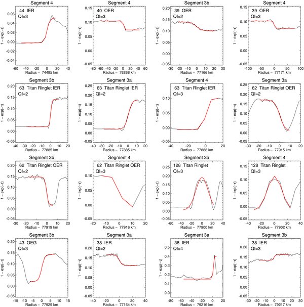
As part of HST program 5824, the 1995 November 21 stellar occultation of GSC 5249-01240 by Saturn's rings was observed in a spectrally resolved mode using the HST's Faint Object Spectrograph. Bosh et al. (2002) used these results, along with earlier occultation data, to determine the orbital characteristics of the inclined, eccentric F ring. However, they published no individual measurements for the rings they used for their geometric solution. Consequently, as with HST 1081, we performed a completely independent analysis of the observations. Figure 2 presents galleries of fits to the detected features, plotted at full resolution (0.2599 s per data point). Once again, the reflex motion of the HST spacecraft resulted in multiple occultation cuts across several ring features; some of the segment numbers have suffixes of a and b, corresponding to the ingress and egress components, respectively, within a given segment.
Download figure:
Standard image High-resolution image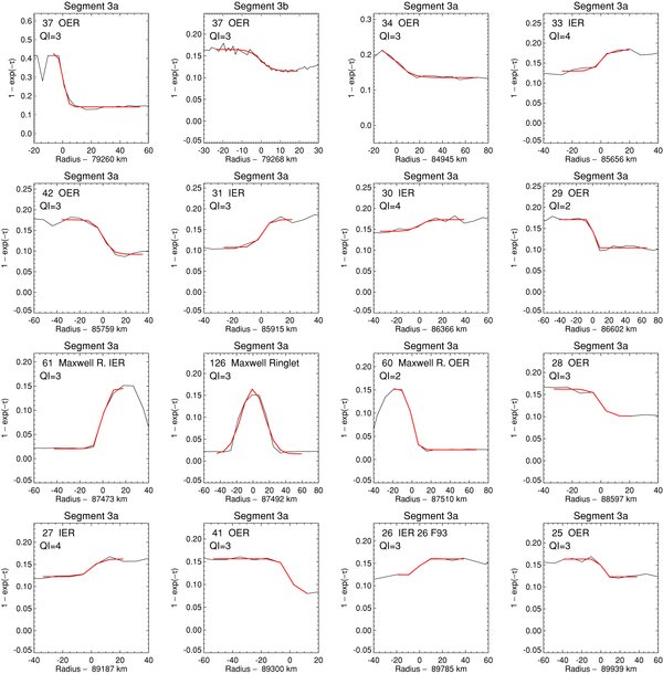
Download figure:
Standard image High-resolution image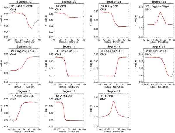
Figure 2. Gallery of ring features from the 1995 November 21 stellar occultation of GSC 5249-01240 observed from the HST under program 5824. Each panel is identified by observation segment number, ring feature number, feature type, and quality index, QI. Each profile is plotted at full resolution (0.2599 s per point) as a function of ring orbital radius. The red curves correspond to the best-fitting logistic model. See Table 4 for details.
Download figure:
Standard image High-resolution imageWe used RINGMASTER to measure the locations of all recognizable ring features, including 24 measurements of 20 presumed-circular rings, and then solved for the event geometry using RINGFIT to determine f0 and g0 as above. Table 4 includes the details of each ring event. The red curves show the best-fitting models to feature edges. The data quality for HST 5824 is generally superior to that of HST 1081, and quite a few profiles were assigned QI = 2 for this occultation. In some instances, we assigned QI = 3 to ring edge measurements of features with poor radial resolution resulting from high ring plane radial velocities, which varied substantially over the course of the occultation. There was a single B-ring outer edge crossing, occurring with a rather high ring plane radial velocity of 54.8 km s−1 due to the co-addition of the HST and Earth orbital motions relative to Saturn at that time. We find that the radius scale from this event is particularly sensitive to the assumed precession rate of Saturn's pole. It will therefore be an important addition to the data sets used to determine the changes in pole orientation over time.
Table 4. HST 5824 Ring Events
| ID | Label | Segment | Observed Time (UTC) | QI | r (km) |  (km s−1) (km s−1) |
λ(°) |
|---|---|---|---|---|---|---|---|
| 44 | IER | 4 | 1995 Nov 21 09:04:55.975 ± 0.036 | 3 | 74495.091 | 25.081 | 325.647 |
| 40 | OER | 4 | 1995 Nov 21 09:06:02.370 ± 0.100 | 3 | 76266.409 | 28.175 | 328.734 |
| 39 | OER | 3b | 1995 Nov 21 07:45:57.391 ± 0.100 | 2 | 77165.592 | 3.203 | 300.032 |
| 4 | 1995 Nov 21 09:06:33.749 ± 0.039 | 3 | 77170.641 | 29.432 | 330.116 | ||
| 63 | Titan Ringlet IER | 3a | 1995 Nov 21 07:38:24.362 ± 0.027 | 2 | 77885.418 | −8.865 | 288.708 |
| 3b | 1995 Nov 21 07:48:59.702 ± 0.017 | 2 | 77885.298 | 4.463 | 302.069 | ||
| 4 | 1995 Nov 21 09:06:57.769 ± 0.011 | 3 | 77888.268 | 30.303 | 331.139 | ||
| 62 | Titan Ringlet OER | 3a | 1995 Nov 21 07:38:21.027 ± 0.050 | 2 | 77915.237 | −9.009 | 288.597 |
| 3b | 1995 Nov 21 07:49:07.157 ± 0.035 | 2 | 77918.646 | 4.488 | 302.120 | ||
| 4 | 1995 Nov 21 09:06:58.695 ± 0.004 | 3 | 77916.349 | 30.335 | 331.178 | ||
| 128 | Titan Ringlet Center | 3a | 1995 Nov 21 07:38:22.740 ± 0.061 | 3 | 77899.856 | −8.935 | 288.654 |
| 4 | 1995 Nov 21 09:06:58.232 ± 0.029 | 3 | 77902.291 | 30.319 | 331.158 | ||
| 43 | OEG | 3b | 1995 Nov 21 07:49:09.469 ± 0.012 | 3 | 77929.030 | 4.496 | 302.136 |
| 39 | IER | 3a | 1995 Nov 21 07:40:12.574 ± 0.074 | 2 | 77164.098 | −4.600 | 292.129 |
| 38 | IER | 3a | 1995 Nov 21 07:36:28.772 ± 0.010 | 4 | 79216.285 | −14.286 | 284.708 |
| 3b | 1995 Nov 21 07:53:43.186 ± 0.091 | 3 | 79216.645 | 4.807 | 302.297 | ||
| 37 | OER | 3a | 1995 Nov 21 07:36:25.698 ± 0.021 | 3 | 79260.462 | −14.441 | 284.598 |
| 3b | 1995 Nov 21 07:53:53.813 ± 0.129 | 3 | 79267.749 | 4.815 | 302.240 | ||
| 34 | OER | 3a | 1995 Nov 21 07:32:01.403 ± 0.090 | 3 | 84945.214 | −28.798 | 274.840 |
| 33 | IER | 3a | 1995 Nov 21 07:31:37.286 ± 0.077 | 4 | 85656.032 | −30.134 | 273.952 |
| 42 | OER | 3a | 1995 Nov 21 07:31:33.873 ± 0.042 | 3 | 85759.221 | −30.322 | 273.827 |
| 31 | IER | 3a | 1995 Nov 21 07:31:28.750 ± 0.057 | 3 | 85915.313 | −30.604 | 273.639 |
| 30 | IER | 3a | 1995 Nov 21 07:31:14.228 ± 0.127 | 4 | 86365.617 | −31.401 | 273.109 |
| 29 | OER | 3a | 1995 Nov 21 07:31:06.736 ± 0.050 | 2 | 86602.446 | −31.810 | 272.837 |
| 61 | Maxwell Ringlet IER | 3a | 1995 Nov 21 07:30:39.995 ± 0.016 | 3 | 87472.652 | −33.258 | 271.870 |
| 126 | Maxwell Ringlet Center | 3a | 1995 Nov 21 07:30:39.416 ± 0.027 | 3 | 87491.931 | −33.289 | 271.849 |
| 60 | Maxwell Ringlet OER | 3a | 1995 Nov 21 07:30:38.880 ± 0.006 | 2 | 87509.781 | −33.318 | 271.829 |
| 28 | OER | 3a | 1995 Nov 21 07:30:07.069 ± 0.051 | 3 | 88596.837 | −35.009 | 270.693 |
| 27 | IER | 3a | 1995 Nov 21 07:29:50.413 ± 0.067 | 4 | 89187.307 | −35.880 | 270.104 |
| 41 | OER | 3a | 1995 Nov 21 07:29:47.287 ± 0.020 | 3 | 89299.744 | −36.042 | 269.995 |
| 26 | IER | 3a | 1995 Nov 21 07:29:33.950 ± 0.001 | 3 | 89785.114 | −36.729 | 269.528 |
| 25 | OER | 3a | 1995 Nov 21 07:29:29.785 ± 0.100 | 3 | 89938.547 | −36.941 | 269.382 |
| 56 | 1.495 RS OER | 3a | 1995 Nov 21 07:29:22.672 ± 0.038 | 3 | 90202.662 | −37.303 | 269.135 |
| 23 | OER | 3a | 1995 Nov 21 07:29:11.586 ± 0.100 | 3 | 90619.360 | −37.862 | 268.752 |
| 55 | B-ring OER | 3a | 1995 Nov 21 07:19:53.896 ± 0.011 | 3 | 117568.109 | −54.638 | 253.408 |
| 122 | Huygens Ringlet Center | 3a | 1995 Nov 21 07:19:49.586 ± 0.011 | 3 | 117803.722 | −54.667 | 253.322 |
| 20 | Huygens Gap OEG | 3a | 1995 Nov 21 07:19:47.184 ± 0.013 | 2 | 117935.046 | −54.682 | 253.273 |
| 4 | Encke Gap IEG | 1 | 1995 Nov 21 05:59:51.460 ± 0.017 | 2 | 133422.183 | −40.061 | 250.380 |
| 3 | Encke Gap OEG | 1 | 1995 Nov 21 05:59:43.297 ± 0.014 | 2 | 133750.842 | −40.442 | 250.264 |
| 2 | Keeler Gap IEG | 1 | 1995 Nov 21 05:58:38.225 ± 0.022 | 3 | 136480.523 | −43.417 | 249.339 |
| 1 | Keeler Gap OEG | 1 | 1995 Nov 21 05:58:37.195 ± 0.018 | 3 | 136525.263 | −43.463 | 249.325 |
| 52 | A ring OER | 1 | 1995 Nov 21 05:58:31.710 ± 0.012 | 2 | 136764.413 | −43.708 | 249.247 |
| 51 | F Ring | 1 | 1995 Nov 21 05:57:18.653 ± 0.003 | 2 | 140075.085 | −46.876 | 248.213 |
Download table as: ASCIITypeset image
4.4. Cassini RSS Observations
The Cassini spacecraft is equipped with an RSS capable of transmitting simultaneously at three wavelengths (λ = 0.9, 3.6, and 13 cm) corresponding to Ka, X, and S bands, respectively (Kliore et al. 2004). Between 2005 May and September, a series of specially designed diametric occultation experiments was conducted, during which the entire ring system was observed along the ansa, provided very high spatial resolution. Unlike the Voyager 1 RSS experiment, which took place at very low ring opening angle, the 2005 diametric occultations were observed when the rings were quite open (|B| = 19°–24°), providing the first high SNR view at radio wavelengths of the high opacity regions of the A and B rings. Four of these occultations were observed during both ingress and egress, resulting in two separate radial scans per occultation (Cassini revs 007, 008, 010, and 012); the remainder were observed only during ingress (rev 014) or egress (revs 009, 011, and 013). All were observed at Ka, X, and S bands, often from multiple antennas at multiple complexes of the Deep Space Network (DSN). For this study, we have used the X-band data only, which have the highest intrinsic SNR. In all, 16 profiles of 12 occultations were uniformly processed to remove the effects of diffraction, with a spatial resolution of 1 km and a sample spacing of 250 m. Figure 3 shows outermost B ring and Cassini Division radial optical depth profile obtained from the rev 007 egress X-band RSS occultation observed from the 70 m DSS-43 station in Canberra, Australia. Note the sharp B-ring outer edge near r = 117,650 km, the multiple sharp-edge ringlets and gaps, and the very stable signal levels in the labeled gaps.
Figure 3. Structure of the outer B ring and Cassini Division. This X-band RSS occultation profile was obtained from the rev 007 egress diametric occultation as recorded at the 70 m DSN station DSS-43. Prominent gaps and ringlets are noted, using the recently adopted IAU nomenclature. Note especially the abrupt outer edge of the B ring, at left, and the quasi-regular spacing of the gaps in the rings.
Download figure:
Standard image High-resolution imageUsing RINGMASTER, we measured the observed event times at each DSN station of all abrupt ringlet and gap edges in all 16 profiles, including most of the features listed in Table II of F93. Then, using the Saturn pole direction and reconstructed Cassini spacecraft trajectory files given in Table 1, we fitted for the equatorial Keplerian orbital elements of 41 ring and gap edges, from a total of 640 individual measurements. (We excluded from the fit several prominent features, including the Titan, Maxwell, and Huygens ringlets and the B-ring edge itself.) Our initial orbit fits showed that there were systematic differences in the ingress and egress orbital radii, for a given Cassini rev, of order 1 km. This is comparable to the estimated uncertainty in the spacecraft location, and since in general the largest component of the trajectory error is in the along-track direction, we included as fitted parameters in our solution the along-track time offsets for each of the 16 occultation profiles. These were typically a few hundredths of a second, and greatly reduced the systematic radius errors.
The rms deviation between the observed and modeled orbital radius was less than 250 m for the majority of the fitted ring edges, a clear indication that most of the ring features are well matched to equatorial Keplerian orbits, and that the intrinsic measurement uncertainty for the RSS ring edge data is on the order of a few hundred meters or less. In cases where we have multiple DSN coverage of a single occultation, we find that the independent measurements of the same ring feature in profiles from different DSN agree to much better than 100 m. That is, noise in the individual observations is not the dominant source of error; more important are the changes in the shape of the ring edge from occultation to occultation, and uncorrected errors in spacecraft position. In Section 5, we describe in more detail the derived orbital characteristics of a number of features in the Cassini Division.
The RSS diametric occultation profiles of the B-ring outer edge provide a high SNR, uniform sample of the opacity profile of the B ring at a variety of longitudes relative to Mimas, all observed with roughly comparable ring opening angle. Figure 4 shows 16 radial profiles from 12 separate occultations, along with superimposed logistic fits to the ring edge. Four of the events include profiles obtained from two separate X-band DSN stations (revs 007 ingress, 009 egress, 011 egress, and 012 egress), showing that the variation in observed edge structure is largely intrinsic to the ring itself, and not primarily due to noise in the observations. Most striking is the strongly varying optical depth of the sharp edge itself, which varies systematically with orbital radius, as shown in Figure 5. Here, we plot the radial variation of the local average of the normal optical depth just interior to the ring edge, as inferred from the logistic fit according to  . The general trend of decreasing optical depth with increasing radius is expected as a result of the transition from compressed streamlines near periapse to more gradual separation near apoapse. The detailed shape of this transition may provide important clues about the internal structure and self-gravity of the inner B ring itself, coupled with an investigation of the detailed structure of the optical depth profiles themselves. We leave this task for a future study.

Figure 4. Cassini RSS occultation profiles of the B-ring outer edge. The radial scale varies from panel to panel because the B-ring edge is not circular. The best-fitting logistic model for each profile is overplotted in red. The quality index, QI, is noted in each panel. We fit the sharp local edge, rather than the broader expanse of the ring structure interior to the edge.
Download figure:
Standard image High-resolution image
Figure 5. Average opacity 〈τ〉 of the extreme outer edge of the B ring as a function of orbital radius. Note the strong variation with radius. The location of the Mimas 2:1 inner Lindblad resonance (r = 117,553 km) is marked with a vertical line.
Download figure:
Standard image High-resolution image5. THE SHAPE OF SATURN'S B RING
The shape of the B ring was first examined in detail by Porco et al. (1984), who used a combination of Voyager images and occultation measurements to show that the observations were largely consistent with a centered elliptical shape with amplitude ae ∼ 74 km rotating at the mean motion of Mimas. They used the presumed constant near-alignment (<10° separation) of the disturbed edge with Mimas and the predicted effects of satellite torque on the ring (Borderies et al. 1982) to estimate the viscosity and velocity dispersion of the outer B ring. They inferred that its maximum height is less than 10 m, although they noted that this depends on the assumed particle size distribution. Bosh (1994) used Voyager 1 and 2, 28 Sgr, and HST 1081 occultation measurements to fit for the shape of the B-ring outer edge, based on their solution for Saturn's pole and precession rate. They found a much smaller amplitude (ae ∼ 23 km) than Porco et al. (1984), which they attributed to not having included the large radius points from Voyager imaging data in their models. Spitale et al. (2006) used Cassini imaging data alone to determine the B ring's shape, finding that at the time of the observations, the periapse of the m = 2 pattern led Mimas by about 28°, although this solution had high residuals. They suggested that an additional m = 3 pattern might also be present. Based on a more extensive survey of Cassini images, Spitale & Porco (2009) have found evidence for chaotic structure in the shape of the B-ring edge. Finally, using VIMS occultation data, Nicholson et al. (2009) and Hedman et al. (2009) found that the angular offset between the ring edge periapse and Mimas seemed to vary in time over the period 2005–2008, although the paucity of VIMS measurements in 2005 made it difficult to establish a unique pattern speed or libration frequency. This lacuna is largely filled with the 2005 RSS occultation measurements reported here, and was the initial motivation for this study.
The complete set of occultation measurements of the B-ring edge considered here is presented in Table 5. For each measurement, we include the event designation, the observing station, the observed time of the ring edge in the recorded occultation curve, the time the occultation ray penetrated the ring plane, the fitted orbital radius, its deviation dr from the mean radius of 117560.930 km of all the occultation measurements, 〈τ〉 for the RSS data only, the longitude λ of the ring intercept point, the longitude of Mimas λ601 at time the ray penetrated the ring plane, and 2(λ − λ601), the relative longitude of the measured feature and Mimas, in an m = 2 frame. In Figure 6, we show the ring radius (expressed in terms of dr) as a function of 2(λ − λ601). The superimposed sine wave shows the Porco et al. (1984) model, based on Voyager results, with the periapse of the ring edge aligned with Mimas (λ = λ601). Note that the Voyager 1 and 2 occultation points lie rather near to the minimum of the sine curve, as expected, since these two measurements were instrumental in supporting the original idea that the periapse of the B-ring edge was aligned with Mimas. The 1989 28 Sgr data are also clustered at radii below the mean radius, with radius residuals in excess of 20 km for the points near 2(λ − λ601) = 20°. A better match to the 28 Sgr data would require a smaller ae of the ring edge, and a phase shift relative to Mimas of about 20°. The two B-ring measurements from the 1991 HST 1081 occultation are far from the model curve, and give strong evidence that the pattern speed of the m = 2 ring edge is not exactly the same as the mean motion of Mimas, as Bosh (1994) also found. The single B-ring measurement from the 1995 HST 5824 occultation is off in 2(λ − λ601) by about 60° from the model, again indicative of a serious problem with the simple idea that the two-lobed pattern is fixed relative to Mimas. Finally, the 2005 RSS data, all obtained within a few months of each other, show a crude match to the m = 2 pattern, but with a phase shift of 2(λ − λ601) ≃ 60° as well. Note that the scatter in the radius of the RSS points, relative to the simple sine wave shape, is not due to measurement uncertainties, which are on the order of only 1 km. Rather, they indicate that the shape of the edge is more complicated than an m = 2 pattern.

Figure 6. Occultation measurements of the radius of the B-ring outer edge, plotted as a function of 2(λ − λMimas). The sinusoidal solid curve corresponds to the Porco et al. (1984) model of the edge as a m = 2 centered ellipse with amplitude ±74 km and periapse aligned with Mimas. The Voyager 1 and 2 points, and perhaps the 28 Sgr data, are consistent with this model, but the 1991 and 1995 HST data deviate strongly from this idealized picture. The RSS diametric occultation measurements from 2005 show an overall m = 2 pattern that is phase-shifted from being aligned with Mimas. Most of the scatter in the results is real; typical measurement uncertainties in the radial location of the B-ring edge are on the order of 1 km. See Table 5 for details.
Download figure:
Standard image High-resolution imageTable 5. Occultation Observations of the B-ring Outer Edge
| Event | Obs | Observed Time (UTC) | UTC at Ring Plane | r (km) | dr (km)a | 〈τ〉 | λ(°) | λ601(°) | 2(λ − λ601)(°) |
|---|---|---|---|---|---|---|---|---|---|
| Voyager 1 | DSS-63 E | 1980 Nov 13 04:54:30.490 | 1980 Nov 13 03:29:44.568 | 117527.754 | −33.176 | 96.716 | 80.265 | 32.903 | |
| Voyager 2 | PPS E | 1981 Aug 26 01:11:22.440 | 1981 Aug 26 01:11:21.715 | 117503.269 | −57.661 | 40.310 | 211.920 | 16.780 | |
| 28 Sgr | PAL I | 1989 Jul 03 06:16:26.670 | 1989 Jul 03 05:01:25.057 | 117522.343 | −38.587 | 32.457 | 7.582 | 49.750 | |
| 28 Sgr | PAL E | 1989 Jul 03 09:10:42.380 | 1989 Jul 03 07:55:40.756 | 117535.368 | −25.562 | 222.470 | 52.882 | −20.824 | |
| 28 Sgr | MCD I | 1989 Jul 03 06:15:39.705 | 1989 Jul 03 05:00:38.093 | 117523.584 | −37.346 | 32.296 | 7.376 | 49.842 | |
| 28 Sgr | MCD E | 1989 Jul 03 09:10:02.177 | 1989 Jul 03 07:55:00.552 | 117534.068 | −26.862 | 222.990 | 52.710 | −19.440 | |
| 28 Sgr | IRTF E | 1989 Jul 03 09:14:03.499 | 1989 Jul 03 07:59:01.879 | 117537.843 | −23.087 | 223.082 | 53.743 | −21.321 | |
| 28 Sgr | ESO 1m I | 1989 Jul 03 06:18:52.260 | 1989 Jul 03 05:03:50.655 | 117526.699 | −34.231 | 25.699 | 8.222 | 34.954 | |
| 28 Sgr | ESO 1m E | 1989 Jul 03 09:11:19.000 | 1989 Jul 03 07:56:17.376 | 117514.732 | −46.198 | 230.336 | 53.039 | −5.406 | |
| 28 Sgr | ESO 2m I | 1989 Jul 03 06:18:52.300 | 1989 Jul 03 05:03:50.695 | 117525.901 | −35.029 | 25.698 | 8.222 | 34.953 | |
| HST 1081 | E | 1991 Oct 03 07:14:26.700 | 1991 Oct 03 05:54:58.687 | 117509.045 | −51.885 | 247.650 | 100.897 | −66.495 | |
| HST 1081 | E | 1991 Oct 03 08:29:48.106 | 1991 Oct 03 07:10:19.683 | 117548.622 | −12.308 | 240.841 | 120.756 | −119.830 | |
| HST 5824 | I | 1995 Nov 21 07:19:53.896 | 1995 Nov 21 06:03:15.693 | 117568.109 | 7.179 | 253.408 | 190.225 | 126.367 | |
| RSS rev 007 | DSS-14 I | 2005 May 03 04:45:16.122 | 2005 May 03 03:27:08.906 | 117494.070 | −66.860 | 3.18 | 259.337 | 63.182 | 32.311 |
| RSS rev 007 | DSS-43 I | 2005 May 03 04:45:16.228 | 2005 May 03 03:27:09.007 | 117494.044 | −66.886 | 2.57 | 259.338 | 63.182 | 32.312 |
| RSS rev 007 | DSS-43 E | 2005 May 03 09:27:51.877 | 2005 May 03 08:09:41.979 | 117646.221 | 85.291 | 0.79 | 60.317 | 135.606 | −150.578 |
| RSS rev 008 | DSS-43 I | 2005 May 21 09:12:27.011 | 2005 May 21 07:52:14.997 | 117579.551 | 18.621 | 0.99 | 257.844 | 166.167 | −176.646 |
| RSS rev 008 | DSS-63 E | 2005 May 21 13:59:07.469 | 2005 May 21 12:38:52.360 | 117563.467 | 2.537 | 0.93 | 62.233 | 241.233 | 1.999 |
| RSS rev 009 | DSS-14 E | 2005 Jun 08 18:47:41.068 | 2005 Jun 08 17:25:39.486 | 117559.674 | −1.256 | 1.01 | 64.276 | 355.948 | 136.656 |
| RSS rev 009 | DSS-63 E | 2005 Jun 08 18:47:40.946 | 2005 Jun 08 17:25:39.353 | 117559.808 | −1.122 | 0.88 | 64.276 | 355.947 | 136.657 |
| RSS rev 010 | DSS-14 I | 2005 Jun 26 19:15:36.753 | 2005 Jun 26 17:52:18.491 | 117530.122 | −30.808 | 2.49 | 253.562 | 39.498 | 68.128 |
| RSS rev 010 | DSS-14 E | 2005 Jun 27 00:11:56.326 | 2005 Jun 26 22:48:36.796 | 117599.827 | 38.897 | 0.72 | 67.130 | 118.272 | −102.286 |
| RSS rev 011 | DSS-43 E | 2005 Jul 15 06:58:44.666 | 2005 Jul 15 05:34:48.771 | 117575.458 | 14.528 | 0.61 | 70.689 | 257.813 | −14.247 |
| RSS rev 011 | DSS-63 E | 2005 Jul 15 06:58:44.907 | 2005 Jul 15 05:34:49.008 | 117575.527 | 14.597 | 0.54 | 70.691 | 257.814 | −14.245 |
| RSS rev 012 | DSS-63 I | 2005 Aug 02 09:50:33.736 | 2005 Aug 02 08:26:39.942 | 117558.831 | −2.099 | 0.89 | 247.446 | 339.569 | 175.755 |
| RSS rev 012 | DSS-14 E | 2005 Aug 02 14:54:26.945 | 2005 Aug 02 13:30:34.729 | 117543.733 | −17.197 | 1.84 | 74.705 | 63.178 | 23.053 |
| RSS rev 012 | DSS-63 E | 2005 Aug 02 14:54:26.792 | 2005 Aug 02 13:30:34.575 | 117543.800 | −17.130 | 1.62 | 74.705 | 63.177 | 23.054 |
| RSS rev 013 | DSS-14 E | 2005 Aug 20 20:37:46.883 | 2005 Aug 20 19:14:33.174 | 117569.182 | 8.252 | 0.55 | 79.570 | 190.242 | 138.657 |
| RSS rev 014 | DSS-14 I | 2005 Sep 05 14:51:58.595 | 2005 Sep 05 13:29:52.384 | 117581.576 | 20.646 | 0.74 | 269.346 | 90.349 | −2.006 |
Note. adr = r − 117560.930 km.
Download table as: ASCIITypeset image
We find that the present data set can be reasonably well matched to a model with an m = 2 component with a slightly different pattern speed from Mimas's mean motion, and an m = 1 component, freely precessing at the rate dictated by Saturn's oblateness. However, because of undersampling, there are multiple solutions for such a model, with roughly comparable statistical significance. Rather than presenting such orbit solutions based on our data alone, we refer the reader to Hedman et al. (2010), who extend the present data set for the B-ring edge by including Cassini VIMS occultation measurements from 2005 to 2009 as well. The ensemble of occultation measurements in Figure 6 spans 25 years, from the Voyager era to the first year of the Cassini orbital tour. By themselves, they show clearly that the B-ring edge is not well matched over that interval by an m = 2 pattern in fixed alignment with Mimas. Although restricted in coverage both in time and in longitude, these data provide important fiducials that any successful model for the B-ring edge must match.
6. CASSINI DIVISION FEATURES
The Cassini Division hosts more than a dozen sharp-edged ringlets and gap edges (Figure 3), most of which are clearly resolved and accurately measurable from occultation profiles. Nicholson et al. (1990) identified many of these, and F93 utilized Voyager and 28 Sgr measurements of a subset of them, presumed to be circular, to establish their geometric solution for Saturn's pole direction and ring plane radius scale. In a separate investigation, Flynn & Cuzzi (1989) compared Voyager images and occultation profiles and concluded that much of the fine-scale structure in the inner Cassini Division was azimuthally symmetric, rather than showing the wake-like features that might be expected from nearby moonlets. Bosh (1994) combined the Voyager, 28 Sgr, and their measurements of HST 1081 features to determine orbits for several non-circular features in the Cassini Division, albeit with rather limited longitude coverage.
Here, we make use of the high spatial resolution, excellent SNR, and rather dense coverage of the rings obtained from the 12 separate 2005 Cassini RSS diametric occultation profiles to examine the orbital characteristics of 16 features in the Cassini Division. Figure 7 is a gallery of the results, showing orbital radius as a function of true anomaly, overplotted in each case with the best-fitting equatorial, Keplerian ellipse. With the exception of two strongly eccentric features, all plots have the same vertical scale for ease of visual comparison of goodness of fit and non-circularity of the orbits. For simplicity, we assumed that the features were precessing freely under the influence of Saturn's J2, J4, and J6, rather than attempting to fit for the precession rate from a data set spanning less than half a year. Table 6 presents the feature ID (expanded from the F93 list), name, fitted semimajor axis a, eccentricity e (expressed for convenience as amplitude ae), the true anomaly ϖ at the epoch UTC 2000 January 1 12:00, the assumed precession rate  , the number of measurements, N, and the rms residual for each feature. The overall radius scale has an uncertainty of just under 2 km, a consequence of allowing for along-trajectory time offsets to be fitted for in the orbit solutions, as described previously in Section 4.4.
Figure 7. Orbit fits to Cassini Division features. The best-fitting precessing, equatorial Keplerian elliptical model for each feature is shown as a sinusoid, plotted as a function of true anomaly. Individual measurements of the edge locations of the features, obtained from 16 RSS occultation profiles, are shown as filled circles. See the text and Table 6 for details.
Download figure:
Standard image High-resolution image
Table 6. Orbit Fits to Cassini Division Features
| ID | Feature | a (km) | ae (km) | ϖ(°) |  (° day−1) (° day−1) |
N | rms (km) | Note |
|---|---|---|---|---|---|---|---|---|
| 20 | Huygens Gap OEG | 117928.85 ± 1.97 | 1.21 ± 0.22 | 61.5 ± 12.8 | 5.00115 | 16 | 0.82 | 1 |
| 19 | Herschel Gap IEG | 118186.77 ± 1.97 | 7.85 ± 0.21 | 115.5 ± 3.2 | 4.96222 | 16 | 0.81 | 1 |
| 18 | 1.960 RS Ringlet IER | 118232.90 ± 1.97 | 1.30 ± 0.21 | 17.8 ± 10.4 | 4.95530 | 16 | 0.56 | 1 |
| 17 | 1.960 RS Ringlet OER | 118261.66 ± 1.97 | 2.34 ± 0.22 | 159.7 ± 6.0 | 4.95099 | 16 | 0.64 | 1 |
| 16 | Herschel Gap OEG | 118281.89 ± 1.97 | 0.88 ± 0.21 | 269.2 ± 15.4 | 4.94797 | 16 | 0.69 | 1 |
| 123 | Russell Gap IEG | 118588.59 ± 1.97 | 8.23 ± 0.23 | 247.8 ± 3.1 | 4.90235 | 16 | 0.17 | 1 |
| 13 | Russell Gap OEG | 118626.91 ± 1.97 | 0.19 ± 0.21 | 326.1 ± 123.9 | 4.89669 | 16 | 0.21 | 2 |
| 15 | Jeffreys Gap OEG | 118965.19 ± 1.97 | 0.25 ± 0.23 | 44.9 ± 58.0 | 4.84707 | 16 | 0.17 | 2 |
| 119 | Kuiper Gap IEG | 119400.12 ± 1.98 | 0.60 ± 0.26 | 154.2 ± 37.4 | 4.78424 | 11 | 0.24 | 2 |
| 118 | Kuiper Gap OEG | 119404.85 ± 1.97 | 0.19 ± 0.21 | 286.8 ± 72.3 | 4.78356 | 16 | 0.20 | 2 |
| 14 | Laplace Ringlet IER | 120035.09 ± 1.97 | 1.76 ± 0.20 | 52.0 ± 7.9 | 4.69438 | 16 | 0.97 | 3 |
| 12 | Laplace Ringlet OER | 120076.38 ± 1.97 | 2.79 ± 0.24 | 357.5 ± 5.0 | 4.68861 | 16 | 0.34 | 1 |
| 127 | Bessel Gap IEG | 120229.58 ± 1.97 | 1.17 ± 0.20 | 81.1 ± 11.8 | 4.66729 | 16 | 0.36 | 1 |
| 11 | Bessel Gap OEG | 120242.33 ± 1.97 | 0.17 ± 0.24 | 32.7 ± 70.8 | 4.66552 | 16 | 0.29 | 2 |
| 10 | Barnard Gap IEG | 120302.11 ± 1.97 | 1.85 ± 0.24 | 263.0 ± 6.9 | 4.65724 | 16 | 1.86 | 4 |
| 9 | Barnard Gap OEG | 120314.58 ± 1.97 | 0.20 ± 0.24 | 197.8 ± 97.3 | 4.65552 | 16 | 0.41 | 2 |
Notes. 1Eccentric feature. 2Circular feature (no measurable eccentricity). 3Significant deviations from Keplerian ellipse. 4Affected by nearby Prometheus 5:4 inner Lindblad resonance.
Download table as: ASCIITypeset image
Several features are measurably eccentric, most notably the Herschel Gap and Russell Gap inner edges (IEG), both of which have amplitudes ae ∼ 8 km. By contrast, the outer edges of the Russell, Jeffreys, Kuiper, Bessel, and Barnard Gaps are conspicuously nearly circular, with ae < 0.25 km in all cases, and rms residuals <0.5 km. The inner edges of these gaps are measurably non-circular, occasionally well matched by a simple precessing ellipse (Kuiper and Bessel Gap IEGs, for example, with rms residuals <0.36 km), but more frequently showing greater scatter. Some of this may be attributable to the ring precessing at a non-Keplerian rate (Hedman et al. 2010), to greater uncertainty in the actual edge measurements for these sometimes rather gradual features, or to significant unmodeled gravitational perturbations in the vicinity of the ring, such as the Prometheus 5:4 ILR in the vicinity of the Barnard Gap IEG. These contributions can most easily be sorted out from the inclusion of a larger set of occultation profiles, which we leave for the future. Nevertheless, there is a clear pattern of generally eccentric, or at least non-circular, inner edges of gaps and nearly circular outer edges of gaps. This systematic pattern was identified by Nicholson et al. (2009) and Hedman et al. (2009), and has been interpreted dynamically by Hedman et al. (2010) as a consequence of forcing by the B ring of a series of regularly spaced resonances, with the gaps opened and maintained by the shepherding action of the non-circular edge of the B ring itself, rather than by as-yet-undetected small moonlets within the gaps.
7. CONCLUSIONS
From both historical and recent occultation observations spanning a quarter of a century, we have obtained 29 precise measurements of the outer edge of the B ring. Beginning with the Voyager 1 RSS and Voyager 2 PPS occultations, and the rich 28 Sgr occultation data set, we adopt a modern value for Saturn's pole direction and precession rate, and use an improved ring orbit model to determine the ring plane radius scale of these early observations. We independently analyzed the observations from two HST occultations, beginning with the 1991 occultation of GSC 6323-01396. As part of this process, we developed a new tool for fitting logistic functions to sharp-edged ring features. Our results are generally in agreement with the E93 measurements of individual ring features from the 1991 HST event, with some exceptions as noted above. We place these data on a consistent radial scale with the rest of our results. Two B-ring edge measurements are provided from this event. We present details of individual measurements of features from the 1995 HST occultation, which will also be useful for helping to determine the precession rate of Saturn's pole from the full set of occultation data. This event adds another B-ring measurement to the set, 10 years prior to the onset of the Cassini orbital tour's occultation sequences. Using a set of 16 high SNR profiles obtained from a sequence of 12 diametric occultations observed at X band by the Cassini RSS team, we obtain measurements of the B-ring edge location at 12 distinct longitudes, showing an approximate m = 2 pattern, but phase shifted relative to Mimas. The early picture of the B-ring edge as permanently aligned with Mimas (Porco et al. 1984) is strongly violated by the ensemble of these observations, indicating that the dynamical picture is considerably more complex than previously imagined.
As part of the global orbital solution for the RSS occultations, we fit Keplerian elliptical orbits to 16 features in the Cassini Division. Several of these are well matched to precessing ellipses; others are nearly circular, in particular the outer edges of gaps, and still others are strongly affected by nearby resonances or other complicating dynamical influences. Collectively, the measurements presented here include the entire historical pre-Cassini occultation survey of the B-ring outer edge, and thus provide an important cross-check for dynamical models of the evolution and variation in the shape of the B ring. The measurements of the Cassini Division features help to characterize the complex range of orbital shapes of ringlets and gaps in a region adjacent to, and probably dynamically affected by, the massive B ring itself. With the inclusion and intercomparison of the full set of Cassini occultation measurements, supplemented by results from Cassini images, a clearer picture of the dynamics and structure of the B ring itself is likely to emerge in the near future.
We thank the members of the Cassini Radio Science Operations Team for their outstanding support in the acquisition of the Cassini RSS occultation observations described in this paper. Phil Nicholson and Matt Hedman provided the impetus for this study. We are grateful to them and to Robert Jacobson and Amanda Bosh for their independent confirmatory calculations of the geometry of several of the occultations. The NAIF team at JPL provided expert guidance in the use of the SPICE toolkit. Amanda Zangari provided programming help, and Team Cassini 2008 members Amanda Curtis, Jillian Garber, Katherine Judd, and David Oakley assisted with the initial data analysis. A very detailed external review by Amanda Bosh is most appreciated. This work was supported in part by the NASA Cassini Data Analysis Program, the NASA Massachusetts Space Grant, the Wellesley College undergraduate summer research program, and the Keck Northeast Astronomy Consortium.
Facilities: HST (FOS, HSP) - Hubble Space Telescope satellite.