

Abstract
Sea ice concentration (SIC) in the eastern Arctic and snow cover extent (SCE) over central Eurasia in late autumn have been proposed as potential predictors of the winter North Atlantic Oscillation (NAO). Here, maximum covariance analysis is used to further investigate the links between autumn SIC in the Barents-Kara Seas (BK) and SCE over Eurasia (EUR) with winter sea level pressure (SLP) in the North Atlantic-European region over 1979-2019. As shown by previous studies, the most significant covariability mode of SIC/BK is found for November. Similarly, the covariability with SCE/EUR is only statistically significant for November, not for October. Changes in temperature, specific humidity, SIC/BK and SCE/EUR in November are associated with a circulation anomaly over the Ural-Siberian region that appears as a precursor of the winter NAO; where the advection of climatological temperature/humidity by the anomalous flow is related to SCE/EUR and SIC/BK anomalies.
Export citation and abstract BibTeX RIS

Original content from this work may be used under the terms of the Creative Commons Attribution 4.0 license. Any further distribution of this work must maintain attribution to the author(s) and the title of the work, journal citation and DOI.
1. Introduction
The North Atlantic Oscillation (NAO) is the most prominent pattern of atmospheric circulation variability in the Euro-Atlantic sector and has a strong influence on the regional surface climate (e.g. Hurrell et al 2003, Hurrell and Deser 2010). Understanding the processes that potentially drive the NAO state is crucial to improve its predictability. Many recent studies have stressed the potential predicting role of eastern Arctic sea ice and continental snow over Eurasia in autumn, with a reduction of sea ice concentration (SIC) in the Barents-Kara Seas and an increase of snow cover extent (SCE) across Siberia that would favor a negative NAO phase during the subsequent winter (e.g. Cohen and Jones 2011, Scaife et al 2014, García-Serrano et al 2015, Dunstone et al 2016, Wang et al 2017).
Sea ice reduction acts as a source of heat and moisture fluxes that can impact both local and large-scale atmospheric circulation. Observational studies (e.g. García-Serrano et al 2015, King et al 2016) and numerical simulations with both atmospheric general circulation models (AGCMs) (e.g. Kim et al 2014, Nakamura et al 2015, Nakamura et al 2016, Sun et al 2015) and coupled climate models (e.g. Kug et al 2015, García-Serrano et al 2017) have found that an anomalous anticyclone over northern Eurasia related to low SIC/BK in late-autumn tends to evolve into a negative NAO-like pattern in winter through a lagged stratospheric pathway. The tropospheric anomalies related to low SIC/BK display a Rossby wave-like anomaly crossing Eurasia, reinforcing the climatological wave pattern. An upward propagation of wave activity finally reaches the stratosphere and weakens the polar vortex. The downward response decelerates the westerlies in the North Atlantic sector shifting the storm-tracks southward, which is tied to a negative NAO phase (e.g. Cohen et al 2014b, Kidston et al 2015). Yet, causality in this chain of processes has to be confirmed (Screen et al 2018, Peings 2019, Blackport et al 2019).
Snow cover variations affect the atmosphere via changes in reflected shortwave solar radiation (albedo), emissivity of longwave radiation, insulation of the atmosphere from the soil layers below, and latent-heat and water release in association with melting (e.g. Cohen and Rind 1991). Observational studies (e.g. Cohen et al 2007) and GCM experiments (e.g. Gong et al 2003a, Gong et al 2003b, Gong et al 2004, Fletcher et al 2007, Fletcher et al 2009, Peings et al 2012, Orsolini et al 2016) showed that an increase in the continental SCE over Eurasia (SCE/EUR) in late autumn can also favor a negative NAO phase in winter via troposphere-stratosphere-troposphere interactions. The mechanism relies on the regional radiative cooling induced by positive SCE anomalies over central Eurasia, which modifies the structure and vertical propagation of planetary-scale wave activity eventually triggering a similar stratospheric pathway as described above. But again, as for SIC/BK, causality related to SCE/EUR has yet to be fully established (Henderson et al 2018, Peings 2019).
The stationarity of the SIC-NAO and SCE-NAO relationships has been questioned (e.g. Kolstad and Screen 2019, Siew et al 2019) due to the shortness of the observational record and the modulation of the polar vortex by the Quasi-Biennal Oscillation (Peings et al 2013, Douville et al 2017). Besides, the connection between these two potential predictors of the winter NAO, i.e. SIC/BK and SCE/EUR, is still an open question (Cohen et al 2014b). Although previous observational and modeling studies have shown that sea-ice reduction over the eastern Arctic is associated with increased snowfall over Siberia (e.g. Deser et al 2010, Cohen et al 2012, Cohen et al 2013, Ghatak et al 2012, Liu et al 2012, Li and Wang 2012, Wegmann et al 2015, Orsolini et al 2016), the physical processes underlying this relationship are unclear. There is also a lack of consensus to determine both the respective contributions of sea-ice and snow-cover anomalies to the winter NAO predictability and the exact timing of their lagged influence on the atmospheric circulation (e.g. Gastineau et al 2017).
The aim of this study is to comprehensively set the observed statistical relationship between SIC/BK and SCE/EUR with the winter NAO and discuss the associated atmospheric circulation, in order to assist model validation in targeted sensitivity experiments to come (Henderson et al 2018, Smith et al 2019). The novelty relies on getting insight into the dynamics underlying the SIC/BK and SCE/EUR anomalies linked to the atmospheric precursor of the winter NAO, namely the Ural-Siberian pattern.
2. Data and Methodology
In this study, empirical orthogonal function (EOF; von Storch and Zwiers 1999) and maximum covariance analysis (MCA; Bretherton et al
1992) are used to describe the spatio-temporal structure of SIC/BK and SCE/EUR variability as well as their covariability with winter sea level pressure (SLP) anomalies over the period 1979-2019. EOF analysis has been employed to test the robustness of the MCA results. The NAO index is defined as the leading principal component (PC), namely standardized time series, corresponding to the leading mode (first EOF) of SLP anomalies in the North-Atlantic-European region (figure 1(a))(NAE:  ; e.g. Hurrell et al (2003)).

Figure 1. (a) Leading EOF of detrended sea level pressure anomalies (hPa) in winter (DJF) over the North Atlantic-European (NAE) region, with a fraction of explained variance of 47.9 % ; note that the negative phase of the NAO is shown. Leading MCA mode between (b) SIC over Barents-Kara Seas (%) and (c) SCE over Eurasia (%) in November with winter (DJF) SLP over the North Atlantic-European region (hPa). Statistically significant areas at 95 % confidence level based on a two-tailed Student's test are contoured. Green contours stand for the climatological sea-ice edge estimated at 15% in (b) and the climatological snow cover edge estimated at 50% in (c); the full field of SIC and SCE climatology can be found in figure S1.
Download figure:
Standard image High-resolution imageMCA is a singular value decomposition (SVD) applied to the covariance matrix of two fields that share a common sampling dimension (the actual time) but can be spatially independent. The output consists of pairs of spatial patterns, each one corresponding to a field, and associated standardized time-series called expansion coefficients (ECs). Each MCA mode is characterized by the squared covariance (sc) which is the eigenvalue of the covariance matrix, the squared covariance fraction (scf) which is a measure of the fraction of explained covariance compared to other modes, and the correlation between the expansion coefficients (cor).
MCA is respectively applied to SIC in the Barents-Kara Seas (BK:  ), and Eurasian SCE (EUR:
  ) for autumn (from September to November) as predictor fields and winter SLP/NAE as predictand field (seasonal average for DJF). The first MCA mode is analyzed in both cases. A Monte Carlo test based on 100 permutations shuffling only the atmospheric field (i.e. SLP) with replacement is performed to determine the statistical significance of these MCA modes. By performing MCA upon each resampling we generate a probability density function (PDF) that is used to compute the significance level (hereafter simply p-value) which corresponds to the number of randomized values (sc, scf or cor) that exceed the actual value being tested (e.g. García-Serrano et al
2015).
) for autumn (from September to November) as predictor fields and winter SLP/NAE as predictand field (seasonal average for DJF). The first MCA mode is analyzed in both cases. A Monte Carlo test based on 100 permutations shuffling only the atmospheric field (i.e. SLP) with replacement is performed to determine the statistical significance of these MCA modes. By performing MCA upon each resampling we generate a probability density function (PDF) that is used to compute the significance level (hereafter simply p-value) which corresponds to the number of randomized values (sc, scf or cor) that exceed the actual value being tested (e.g. García-Serrano et al
2015).
Monthly SIC data are provided by HadISST (Hadley Center Sea Ice and Sea Surface Temperature; Rayner et al
2003) at  resolution and SCE data from the Global Snow Laboratory at Rutgers University (Robinson et al
1993). For SCE, October is defined as the average of the calendar weeks 40-44 (Cohen and Jones 2011), and November of the weeks 44-48. Compared to Peings et al (2013) for SCE and García-Serrano et al (2015) for SIC, our choice of dataset does not affect results. Monthly data of atmospheric variables are given by ERA-Interim reanalysis available from the European Center for Medium-Range Weather Forecasts (ECMWF) at
resolution and SCE data from the Global Snow Laboratory at Rutgers University (Robinson et al
1993). For SCE, October is defined as the average of the calendar weeks 40-44 (Cohen and Jones 2011), and November of the weeks 44-48. Compared to Peings et al (2013) for SCE and García-Serrano et al (2015) for SIC, our choice of dataset does not affect results. Monthly data of atmospheric variables are given by ERA-Interim reanalysis available from the European Center for Medium-Range Weather Forecasts (ECMWF) at  resolution (Dee et al
2011). Forecast-accumulated turbulent (sensible plus latent) and radiative (shortwave plus longwave) heat fluxes initialized twice a day (00, 12 h) from ERA-Interim are also used; upward is positive, from surface to atmosphere. All anomalies are detrended before analysis to focus on the interannual variability, aiming to exclude any long-term relationship among variables. Different detrending methods (1st-, 2nd- and 3th-order polynomial fits) have been evaluated to assess robustness of the results; in the manuscript we only show cubicly detrended anomalies because of the strong non-linear trends in SIC/BK, but the results are largely insensitive to the detrending method.
resolution (Dee et al
2011). Forecast-accumulated turbulent (sensible plus latent) and radiative (shortwave plus longwave) heat fluxes initialized twice a day (00, 12 h) from ERA-Interim are also used; upward is positive, from surface to atmosphere. All anomalies are detrended before analysis to focus on the interannual variability, aiming to exclude any long-term relationship among variables. Different detrending methods (1st-, 2nd- and 3th-order polynomial fits) have been evaluated to assess robustness of the results; in the manuscript we only show cubicly detrended anomalies because of the strong non-linear trends in SIC/BK, but the results are largely insensitive to the detrending method.
To explore the dynamics involved in the statistical relationships, regression maps are computed by projecting different anomalous fields onto a time-series, either the NAO index or the MCA expansion coefficients. In this case, the statistical significance of the regressed anomalies is evaluated with a two-tailed Students t-test at 95% confidence level.
3. Results
3.1. Covariability: SIC/BK and SCE/EUR
The leading MCA mode based on September SIC/BK anomalies explains 58% of scf (p-value 29%), with a sc of  (p-value 16%) and yields a cor of 0.56 (p-value 27%)(table 1). These high p-values indicate a low confidence level for this relationship, associated with a low signal-to-noise ratio and non-significant predictability (e.g. García-Serrano et al
2015, Koenigk et al
2016). For October, the leading MCA mode explains 85% of scf (p-value 1%), with a sc of
(p-value 16%) and yields a cor of 0.56 (p-value 27%)(table 1). These high p-values indicate a low confidence level for this relationship, associated with a low signal-to-noise ratio and non-significant predictability (e.g. García-Serrano et al
2015, Koenigk et al
2016). For October, the leading MCA mode explains 85% of scf (p-value 1%), with a sc of  (p-value 0%), and yields a cor of 0.60 (p-value 3%)(table 1). The leading MCA mode based on November SIC/BK anomalies explains 82% of scf (p-value 2%), with a sc of
  (p-value 0%) and yields a cor of 0.63 (p-value 1%)(table 1). The MCA-SIC/BK in October is also significant, but there is no clear atmospheric mechanism responsible for a lagged relationship with the winter NAO (see García-Serrano et al
2015). According to King and García-Serrano (2016), the potential influence of October SIC/BK anomalies on the winter Euro-Atlantic climate would rely on its contribution to November SIC/BK anomalies. On the other hand, the dynamics associated with SIC/BK anomalies in November are much more plausible and largely reported. It could involve a stratospheric pathway (e.g. Nakamura et al
2015, Nakamura et al
2016, King et al
2016) and represent a suitable predictability source of the winter Euro-Atlantic climate (e.g. Scaife et al
2014, García-Serrano et al
2015, Koenigk et al
2016, Dunstone et al
2016). Thereby, the analysis is focused hereafter on November SIC/BK variability. To simplify the nomenclature, we will refer to the MCA covariability mode between SIC/BK in November and SLP/NAE in winter as
(p-value 0%) and yields a cor of 0.63 (p-value 1%)(table 1). The MCA-SIC/BK in October is also significant, but there is no clear atmospheric mechanism responsible for a lagged relationship with the winter NAO (see García-Serrano et al
2015). According to King and García-Serrano (2016), the potential influence of October SIC/BK anomalies on the winter Euro-Atlantic climate would rely on its contribution to November SIC/BK anomalies. On the other hand, the dynamics associated with SIC/BK anomalies in November are much more plausible and largely reported. It could involve a stratospheric pathway (e.g. Nakamura et al
2015, Nakamura et al
2016, King et al
2016) and represent a suitable predictability source of the winter Euro-Atlantic climate (e.g. Scaife et al
2014, García-Serrano et al
2015, Koenigk et al
2016, Dunstone et al
2016). Thereby, the analysis is focused hereafter on November SIC/BK variability. To simplify the nomenclature, we will refer to the MCA covariability mode between SIC/BK in November and SLP/NAE in winter as  .
.
Table 1. Results of the MCA covariability analysis between autumn SIC/BK and SCE/EUR with winter SLP/NAE for the period 1979-2019. The squared covariance fraction (scf), the squared covariance (sc) and the correlation between the expansion coefficients (cor) are listed for each mode, together with the significance level (p-value).
| September | October | November | |
|---|---|---|---|
( ) ) | |||
| scf (p-value) | 58 % (29%) | 85 % (1%) | 82% (2%) |
| sc (p-value) | 1.35 × 10⁷(16 %) | 5.09× 10⁷(0%) | 3.53 × 10⁷ (0%) |
| cor (p-value) | 0.56 (27 %) | 0.60 (3%) | 0.63 (2%) |
( ) ) | |||
| scf (p-value) | / | 52 % (45%) | 74 % (0%) |
| sc (p-value) | / | 1.90 × 10⁷(26%) | 4.89 × 10⁷ (0%) |
| cor (p-value) | / | 0.69 (33%) | 0.76 (13%) |
Figure 1(b) shows the regression map of SIC anomalies in November onto the SIC expansion coefficient of  . The resulting SIC pattern shows negative anomalies (i.e. sea-ice reduction) over the northern Barents Sea and the whole Kara Sea. The SLP covariability pattern of
  (not shown) strongly resembles the negative phase of the NAO (figure 1(a)). The SLP expansion coefficient of
  has indeed a correlation of -0.99 with the winter NAO index, illustrating that the NAO has been effectively captured as predictand.
Caution is required to assert cause and effect based on observational data and MCA results. Concerning the former, several studies using AGCM simulations (e.g. Nakamura et al
2015, Nakamura et al
2016, Sun et al
2015) have also found a lagged teleconnection between SIC/BK anomalies and the NAO, although the timing may be model dependent (García-Serrano et al
2017). As for the latter, we further explore the suitability of SIC/BK as predictor. The SIC expansion coefficient of  is compared with the leading principal component (PC1) of SIC over the eastern Arctic and over the Northern Hemisphere in November: the SIC expansion coefficient yields a high correlation with both the regional PC1 (0.98) and the hemispheric PC1 (0.93). Likewise, the lagged regressions of winter SLP onto the two PC1s are almost identical to that of the SIC expansion coefficient (not shown), which is consistent with alternative approaches based on area-averaged SIC indices (Koenigk et al
2016, King et al
2016). Hence, the covariability mode of
is compared with the leading principal component (PC1) of SIC over the eastern Arctic and over the Northern Hemisphere in November: the SIC expansion coefficient yields a high correlation with both the regional PC1 (0.98) and the hemispheric PC1 (0.93). Likewise, the lagged regressions of winter SLP onto the two PC1s are almost identical to that of the SIC expansion coefficient (not shown), which is consistent with alternative approaches based on area-averaged SIC indices (Koenigk et al
2016, King et al
2016). Hence, the covariability mode of  is associated with a leading mode of SIC variability per se. Note that the SIC pattern of
  corresponds to the second EOF of turbulent heat flux in Sorokina et al (2016), with a strong ocean-to-atmosphere forcing (see also García-Serrano et al
2015 and Yang et al
2016); which is unrelated to the so-called 'Warm Arctic-Cold Siberia' (WACS) pattern in winter. It follows that November SIC/BK anomalies can be considered as a potential predictor of the subsequent winter NAO. Lagged regression of SIC anomalies in November onto the winter NAO index (figure S2a (https://stacks.iop.org/ERL/15/124010/mmedia)) support this conclusion.
corresponds to the second EOF of turbulent heat flux in Sorokina et al (2016), with a strong ocean-to-atmosphere forcing (see also García-Serrano et al
2015 and Yang et al
2016); which is unrelated to the so-called 'Warm Arctic-Cold Siberia' (WACS) pattern in winter. It follows that November SIC/BK anomalies can be considered as a potential predictor of the subsequent winter NAO. Lagged regression of SIC anomalies in November onto the winter NAO index (figure S2a (https://stacks.iop.org/ERL/15/124010/mmedia)) support this conclusion.
Analogous to the procedure followed for SIC/BK, MCA based on SCE/EUR anomalies in late autumn (October, November) have been performed. Note that September has not been considered because there is almost no snow cover over the continent at that time of the year (e.g. Han and Sun 2018). The leading MCA mode for October SCE/EUR anomalies explains 52% of scf (p-value 45%), with a sc of 1.90 × 10⁷(p-value 26%), and yields a cor of 0.69 (p-value 33%). For November, the leading MCA explains 74% of scf (p-value 0%), with a sc of 4.89 × 10⁷(p-value 0%) and yields a cor of 0.76 (p-value 13%). Extending the period using reanalyzed SCE data (instead of satellite-derived products) would probably not lead to better statistical results (Peings et al 2013) especially when considering the potential non-stationarity of the snow-NAO relationship (Douville et al 2017). In contrast to previous studies that suggested a statistically significant relationship between October SCE/EUR and the winter NAO (e.g. Cohen et al 2001, 2002, 2007), these results reveal that the covariability of October SCE/EUR with winter SLP/NAE is largely statistically non-significant, namely not discernable from noise. However, we found that November SCE/EUR anomalies tend to be followed by NAO-like atmospheric variability, a result consistent with the monthly analysis of Gastineau et al (2017).
This finding is supported by the lagged regression maps of autumn SCE/EUR anomalies onto the winter NAO index, where October does not show statistically significant anomalies over Eurasia (not shown) but November does so (figure S2b). Thus, in the following the analysis is restricted to November SCE/EUR. As for SIC, we will refer to the leading MCA covariability mode between SCE/EUR in November and SLP/NAE in winter as  for the sake of readability. Figure 1(c) shows the covariability mode of SCE from
  , exhibiting statistically significant positive anomalies (i.e. snow cover increase) over central-eastern Eurasia. The SLP covariability of
  displays a negative NAO-like pattern (not shown, but similar to figure 1(a)) and its expansion coefficient correlates at -0.99 with the winter NAO index.
The SCE expansion coefficient of  attains only a correlation of 0.58 (0.30) with the first (second) EOF of November SCE/EUR. The fraction of explained variance of the two leading EOFs is very low (EOF1 = 15%, EOF2 = 12%), indicating that they are not well separated statistically (following North et al
1982) and illustrating that SCE is a noisy field. This result implies, as opposed to the case of November SIC/BK, that the covariability of
attains only a correlation of 0.58 (0.30) with the first (second) EOF of November SCE/EUR. The fraction of explained variance of the two leading EOFs is very low (EOF1 = 15%, EOF2 = 12%), indicating that they are not well separated statistically (following North et al
1982) and illustrating that SCE is a noisy field. This result implies, as opposed to the case of November SIC/BK, that the covariability of  does not rely on a dominant variability mode of snow cover itself, which questions the feasibility of using SCE/EUR as a potential predictor for the NAO.
Repeating the analysis with snow depth (SD) from ERA-Interim yields consistent results: namely, the MCA with October SD not being significant and the one with November SD showing hints of significance. In the latter case, as opposed to using satellite-derived SCE, sc and scf are higher but above 10% significance level, while the correlation between expansion coefficients is smaller but significant at 3% (cor = 0.52). The  pattern (not shown) and the regression of November SD/EUR anomalies onto the winter NAO index (figure S3) display positive anomalies over central Eurasia, particularly west of the Baikal Lake.
3.2. Ural-Siberian anticyclone (SCAND)
To shed light on the large-scale atmospheric circulation in November preceding the winter NAO, the climatology and variability of SLP over Eurasia is analysed. This is compared to contemporaneous SLP anomalies associated with  and
and  , together with the SLP precursor of the NAO obtained by regressing November SLP anomalies onto the winter NAO index.
Figure 2(b) shows the regression map of Northern Hemisphere (NH) SLP anomalies onto the first EOF of November SLP anomalies over Eurasia ( ; EOF1). This regional EOF1 strongly resembles the hemispheric EOF1 (not shown; r = 0.89), which is also a dominant mode of variability later in the season - in winter (Smoliak and Wallace 2015). The pattern is dominated by an anticyclonic circulation anomaly over the subarctic Eurasian region, but exhibits a dipole-like structure with a weaker center of opposite sign over western Europe. The identification of this surface anticyclone has been ambiguous in the literature. It appears to be related to Ural blocking at daily time-scales (e.g. Mori et al
2014, Tyrlis et al
2019), but it also constitutes a prominent mode of variability at monthly and seasonal time-scales (e.g. García-Serrano et al
2017, Peings 2019). Smoliak and Wallace (2015) tentatively named it as the Russian (RU) pattern, but here it will be referred to as the Ural-Siberian (U-S) pattern. Interestingly, the centers of action of EOF1 (figure 2(b)) tightly project on the areas of maximum interannual variability (i.e. standard deviation; green contours in figure 2(a)), as it is also the case for the mid- (500hPa; King et al
2018) and upper-tropospheric (200hPa; García-Serrano et al
2017) geopotential height. The leading mode of Eurasian geopotential height variability in the mid-upper troposphere, which has a better-defined wave-like signature (figure S4a at 300hPa; e.g. García-Serrano et al
2017), can be more easily identified as the Scandinavian (SCAND) pattern, a mode of internal variability associated with Rossby wave propagation dynamics and maintained by transient-eddy feedback (e.g. Bueh and Nakamura 2007, Liu et al
2014). Note that the U-S pattern of SLP corresponds to the surface projection of the SCAND pattern at upper levels, and the other way around, since they show a marked barotropic structure (e.g. Liu et al
2014, Smoliak and Wallace 2015).
; EOF1). This regional EOF1 strongly resembles the hemispheric EOF1 (not shown; r = 0.89), which is also a dominant mode of variability later in the season - in winter (Smoliak and Wallace 2015). The pattern is dominated by an anticyclonic circulation anomaly over the subarctic Eurasian region, but exhibits a dipole-like structure with a weaker center of opposite sign over western Europe. The identification of this surface anticyclone has been ambiguous in the literature. It appears to be related to Ural blocking at daily time-scales (e.g. Mori et al
2014, Tyrlis et al
2019), but it also constitutes a prominent mode of variability at monthly and seasonal time-scales (e.g. García-Serrano et al
2017, Peings 2019). Smoliak and Wallace (2015) tentatively named it as the Russian (RU) pattern, but here it will be referred to as the Ural-Siberian (U-S) pattern. Interestingly, the centers of action of EOF1 (figure 2(b)) tightly project on the areas of maximum interannual variability (i.e. standard deviation; green contours in figure 2(a)), as it is also the case for the mid- (500hPa; King et al
2018) and upper-tropospheric (200hPa; García-Serrano et al
2017) geopotential height. The leading mode of Eurasian geopotential height variability in the mid-upper troposphere, which has a better-defined wave-like signature (figure S4a at 300hPa; e.g. García-Serrano et al
2017), can be more easily identified as the Scandinavian (SCAND) pattern, a mode of internal variability associated with Rossby wave propagation dynamics and maintained by transient-eddy feedback (e.g. Bueh and Nakamura 2007, Liu et al
2014). Note that the U-S pattern of SLP corresponds to the surface projection of the SCAND pattern at upper levels, and the other way around, since they show a marked barotropic structure (e.g. Liu et al
2014, Smoliak and Wallace 2015).
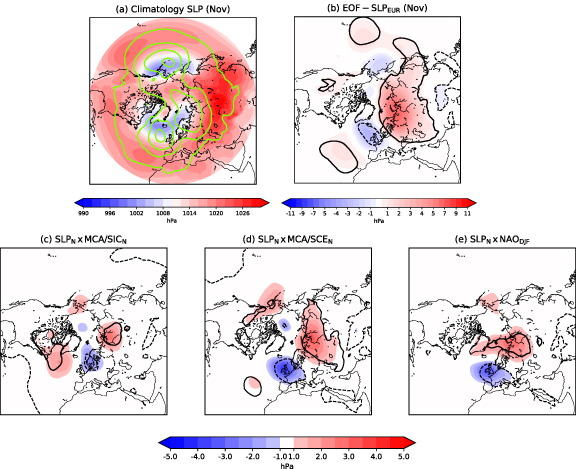
Figure 2. (a) Climatology (hPa ; shading) and standard deviation (ci = 2hPa ; green contours) of SLP in November. Regression map of detrended Northern Hemisphere sea level pressure anomalies (hPa) in November onto (b) the leading PC from the EOF analysis of November SLP over Eurasia ( N,
N,  E ; 41.5 % fraction of explained variance), (c) the
  expansion coefficient, (d) the
  expansion coefficient and (e) the winter NAO index - multiplied by -1. Statistically significant areas at 95 % confidence level based on a two-tailed Student's test are contoured.
Download figure:
Standard image High-resolution imageThe statistically significant SLP anomalies preceding the winter NAO also show a dipole-like structure (figure 2(e)), projecting on the centers of the U-S pattern over the Siberian coast and the British Isles (figure 2(b)). At 300hPa, the winter NAO is preceded by a wave-like structure over Eurasia, which also projects on the SCAND pattern at upper levels (figure S4c). These results are consistent with Kuroda and Kodera (1999), Takaya and Nakamura (2008), Orsolini et al (2011) and García-Serrano et al (2015) who showed that the winter NAO tends to be preceded by a wave-like anomaly over Eurasia, which triggers a stratospheric pathway. These findings suggest that the U-S/SCAND pattern in November may eventually evolve into the winter NAO with a 1-month lead time and might be considered a precursor of the winter NAO. This line of reasoning has been recently confirmed by Peings (2019).
Figures 2(c) and (d) show the regression map of contemporaneous SLP anomalies onto expansion coefficients of SIC and SCE from  and
and  , respectively. The anomalous dipole-like pattern associated with
  (figure 2(d)) has a strong resemblance to EOF1 (figure 2(b)), which is consistent with previous studies using other autumnal Eurasian SCE indices (e.g. Cohen et al
2001, 2014a). It is worth noting that there is no signal over the Siberian High region (reddest areas at mid-latitudes of figure 2(a)), which would be expected from the radiative feedback linked to Eurasian snow cover anomalies (figure 1(c) and S2b). However, the anomalous Ural-Siberian anticyclone in figure 2(b) has been usually interpreted as a north-westward expansion of the Siberian High in response to increased SCE over central Eurasia (Cohen et al
2001, 2002, 2007, 2010, 2014a), although the U-S pattern develops over the subpolar low-pressure belt along the Siberian coast (blue shading in figure 2(a)), linked to local transient-eddy activity (e.g. Vallis and Gerber 2008) and cyclone tracks (e.g. Inoue et al
2012). In fact, no AGCM study prescribing positive Eurasian SCE anomalies has reported such a circulation response. Instead, they have found a regional baroclinic structure associated with a reinforced Siberian High at surface and cyclonic circulation anomalies in the upper troposphere (Gong et al
2003a, 2003b, 2004, Fletcher et al
2007, 2009, Orsolini and Kvamstø 2009, Allen and Zender 2010, Peings et al
2012); the most significant being the reinforcement of the Siberian High (Henderson et al
2018, Peings 2019). Thus, there is no modelling evidence supporting the impact or triggering role of SCE/EUR anomalies on the U-S/SCAND pattern. This line of reasoning suggests that the SCE/EUR anomalies in November related to the winter NAO (figure 1(c) and S2b) might be potentially driven by the Ural-Siberian anticyclone (figure 2(b)) rather than the other way around, which is in agreement with Henderson et al (2018) and Peings (2019) and further discussed in section 3.4.
(figure 2(d)) has a strong resemblance to EOF1 (figure 2(b)), which is consistent with previous studies using other autumnal Eurasian SCE indices (e.g. Cohen et al
2001, 2014a). It is worth noting that there is no signal over the Siberian High region (reddest areas at mid-latitudes of figure 2(a)), which would be expected from the radiative feedback linked to Eurasian snow cover anomalies (figure 1(c) and S2b). However, the anomalous Ural-Siberian anticyclone in figure 2(b) has been usually interpreted as a north-westward expansion of the Siberian High in response to increased SCE over central Eurasia (Cohen et al
2001, 2002, 2007, 2010, 2014a), although the U-S pattern develops over the subpolar low-pressure belt along the Siberian coast (blue shading in figure 2(a)), linked to local transient-eddy activity (e.g. Vallis and Gerber 2008) and cyclone tracks (e.g. Inoue et al
2012). In fact, no AGCM study prescribing positive Eurasian SCE anomalies has reported such a circulation response. Instead, they have found a regional baroclinic structure associated with a reinforced Siberian High at surface and cyclonic circulation anomalies in the upper troposphere (Gong et al
2003a, 2003b, 2004, Fletcher et al
2007, 2009, Orsolini and Kvamstø 2009, Allen and Zender 2010, Peings et al
2012); the most significant being the reinforcement of the Siberian High (Henderson et al
2018, Peings 2019). Thus, there is no modelling evidence supporting the impact or triggering role of SCE/EUR anomalies on the U-S/SCAND pattern. This line of reasoning suggests that the SCE/EUR anomalies in November related to the winter NAO (figure 1(c) and S2b) might be potentially driven by the Ural-Siberian anticyclone (figure 2(b)) rather than the other way around, which is in agreement with Henderson et al (2018) and Peings (2019) and further discussed in section 3.4.
On the other hand, the dipole-like pattern of SLP anomalies associated with  (figure 2(c)) is slightly different from the other patterns, as the centers of action are located downstream, with the anticyclonic anomalies shifted toward the continent and the cyclonic anomalies displaced toward the Nordic Seas. The vertical structure of the anticyclonic anomalies over the Siberian coast reveals some baroclinicity (cf figure S4a), in agreement with AGCM simulations (e.g. Honda et al
2009), which suggests a possible contribution of SIC/BK variability on the U-S pattern (García-Serrano et al
2015) that is further discussed in section 3.4.
(figure 2(c)) is slightly different from the other patterns, as the centers of action are located downstream, with the anticyclonic anomalies shifted toward the continent and the cyclonic anomalies displaced toward the Nordic Seas. The vertical structure of the anticyclonic anomalies over the Siberian coast reveals some baroclinicity (cf figure S4a), in agreement with AGCM simulations (e.g. Honda et al
2009), which suggests a possible contribution of SIC/BK variability on the U-S pattern (García-Serrano et al
2015) that is further discussed in section 3.4.
3.3. Linkage between SIC/BK and SCE/EUR
To explore the relationship between November SIC/BK and SCE/EUR in relation to the winter NAO, regional near-surface conditions of temperature (T925), specific humidity (q925) and horizontal wind are analyzed at 925hPa (figure 3). As our framework does not allow disentangling cause and effect, the analysis below is focused on lagged regressions in November onto the winter NAO index, thereby assessing the observed NAO precursors in an objective way. Regressions onto the expansion coefficients of  or
or  yield very similar results.
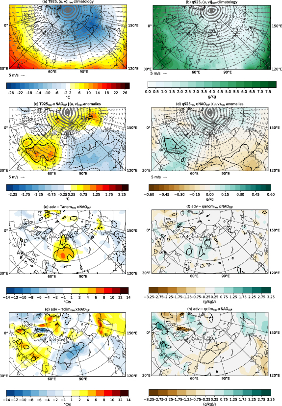
Figure 3. (a), (b) Climatology of November air temperature (T925 ;  C ) and specific humidity (q925 ; g kg−1). Climatological wind at 925 hPa (
 ; m s−1) is overplotted with vectors. (c), (d) Regression map of detrended T925 (
 C) and q925 (g kg−1) anomalies in November onto the winter NAO index-multiplied by -1. Anomalous wind at 925hPa (u',v'; m s−1) is overplotted with vectors. (e,f) Regression map of the advection of anomalous T925 (
 C s−1) and q925 ((g kg−1)/s) by the climatological flow in November onto the winter NAO index - multiplied by -1. (g), (h) Regression map of the advection of climatological T925 (
 C s−1) and q925 ((g kg−1)/s) by the anomalous flow in November onto the winter NAO index - multiplied by -1.
Download figure:
Standard image High-resolution imageClimatology in this region shows a cold and dry environment east of Scandinavia (eastern Arctic/eastern Siberia), whereas in western Europe warm and wet conditions prevail (figures 3(a) and (b)). Figures 3(c) and (d) show regression maps of November T925 and q925 onto the winter NAO index, respectively. Warm and wet anomalies are found over the Barents-Kara Seas in relation to sea-ice reduction (c.f. figures 1(b), S2a) while cold and dry anomalies extend across Eurasia in association with the increase in snow cover (c.f. figures 1(c), S2b), although only the latter is statistically significant. SIC/BK reduction and SCE/EUR increase are source and sink of humidity, respectively, as discussed in previous observational and modelling studies (e.g. Liu et al 2012, Li and Wang 2012, Wegmann et al 2015). Noteworthy, it is usually assumed that the connection between SIC/BK and SCE/EUR is as follows: sea-ice reduction providing extra evaporation, increased moisture flux inland, and enhanced snowfall over Eurasia (e.g. Cohen et al 2014a, Tyrlis et al 2019). However, model results show that the direct impact of sea-ice reduction on snowfall would mainly apply to the Siberian coast (e.g. Deser et al 2010, Ghatak et al 2012, Orsolini et al 2012). Hence, there is room for further exploring the winter NAO-related SIC/BK and SCE/EUR anomalies.
The target diagnostics are the linear advection terms of T925 and q925: namely, the advection of climatological T925/q925 by the anomalous flow [ ] and the advection of anomalous T925/q925 by the climatological flow [
 ]; the non-linear advection terms are negligible in terms of amplitude (not shown) (e.g. Wallace and Hobbs 2006). The advection of anomalous T925/q925 driven by the southwesterly climatological flow (figures 3(e) and (f)), bringing warm and wet air masses from the Mediterranean, yield statistically significant anomalies upstream and over the Ural Mountains, i.e. windward. These warm and wet conditions do not contribute to the snow dipole preceding the NAO shown on figure 1(c). On the other hand, the advection of climatological T925/q925 by the anomalous flow yield statistically significant anomalies downstream (downwind) the Urals, namely over Siberia (figures 3(g) and (h)). It implies that the wind anomalies preceding the NAO transport cold and dry air from the Arctic into Eurasia, indicative of land cooling and humidity sink associated with snowfall, particularly west of Baikal Lake (cf figures 1(c), S3). This south-eastward transport, together with the induced warm and wet advection over the Mediterranean region (figure 3(g) and (h)), suggests that the anomalous U-S anticyclone is the responsible of pushing the snow edge northward over western Eurasia and southward over eastern Eurasia, thereby generating the anomalous continental-scale dipole of snow cover (figure 1(c)) and surface conditions (figure 3(c) and (d)). These results contrast with previous works suggesting that increased SCE/EUR is a consequence of the moisture increase due to SIC/BK reduction (e.g. Cohen et al
2012, Wegmann et al
2015), since our results suggest that the relationship is determined by the advection of climatological cold air from the Arctic, mediated by the anomalous atmospheric circulation.
]; the non-linear advection terms are negligible in terms of amplitude (not shown) (e.g. Wallace and Hobbs 2006). The advection of anomalous T925/q925 driven by the southwesterly climatological flow (figures 3(e) and (f)), bringing warm and wet air masses from the Mediterranean, yield statistically significant anomalies upstream and over the Ural Mountains, i.e. windward. These warm and wet conditions do not contribute to the snow dipole preceding the NAO shown on figure 1(c). On the other hand, the advection of climatological T925/q925 by the anomalous flow yield statistically significant anomalies downstream (downwind) the Urals, namely over Siberia (figures 3(g) and (h)). It implies that the wind anomalies preceding the NAO transport cold and dry air from the Arctic into Eurasia, indicative of land cooling and humidity sink associated with snowfall, particularly west of Baikal Lake (cf figures 1(c), S3). This south-eastward transport, together with the induced warm and wet advection over the Mediterranean region (figure 3(g) and (h)), suggests that the anomalous U-S anticyclone is the responsible of pushing the snow edge northward over western Eurasia and southward over eastern Eurasia, thereby generating the anomalous continental-scale dipole of snow cover (figure 1(c)) and surface conditions (figure 3(c) and (d)). These results contrast with previous works suggesting that increased SCE/EUR is a consequence of the moisture increase due to SIC/BK reduction (e.g. Cohen et al
2012, Wegmann et al
2015), since our results suggest that the relationship is determined by the advection of climatological cold air from the Arctic, mediated by the anomalous atmospheric circulation.
3.4. Causality between SIC/BK, SCE/EUR and the U-S pattern
To gain insight on the causality between SIC/BK, SCE/EUR and the regional atmospheric circulation, turbulent (THF; sensible (SHF) plus latent (LHF)) and radiative (RHF; shortwave (SWR) plus longwave (LWR)) surface heat fluxes in November are analyzed (figure 4).

Figure 4. Regression map of detrended turbulent heat flux anomalies ( ; (a), (c), (e), (g)) and radiative heat flux anomalies (
 ; b,d,f,h) in November onto (a), (b) the leading PC from the EOF analysis of November SLP over Eurasia (see figure 2(b)), (c), (d) the
  expansion coefficient, (e), (f) the
  expansion coefficient and (g), (h) the winter NAO index—multiplied by -1. Statistically significant areas at 95 % confidence level based on a two-tailed Student's test are contoured.
Download figure:
Standard image High-resolution image
Over the ocean, THF anomalies associated with the U-S pattern are dominated by downward heat flux, that is by ocean heat uptake, over the Norwegian Sea and the southern, ice-free Barents Sea (figure 4(a)). These negative THF anomalies are likely related to the southerly advection of warm and moist air induced by the anticyclonic circulation in the Siberian coast and the cyclonic circulation over the British Isles (figure 2(b)); note that both SHF and LHF anomalies contribute almost equally (figure S5). This anomalous THF pattern strongly resembles the atmosphere-driven THF EOF1 of Sorokina et al (2016). And, consistently with this interpretation, the U-S/SCAND mode also shows negative RHF anomalies (figure 4(b)), which are determined by increased downwelling LWR (figure S6; e.g. Blackport et al
2019, and references therein). On the other hand, THF anomalies associated with  display enhanced upward heat flux over the Kara Sea and northern Barents Sea (figure 4(c)). These positive THF anomalies, with contribution from both SHF and LHF (figure S5), are related to sea-ice reduction and its retreat of the edge (figure 1(b)). In this case, the anomalous THF pattern projects on the ice-driven THF EOF2 of Sorokina et al (2016), associated with heat release over the newly-opened oceanic area (e.g. Blackport et al
2019). Note that this positive THF anomaly over BK is accompanied by a negative THF anomaly sharply south of the sea-ice edge (cf figures 1(b), 4(c)), which is the expected response to sea-ice reduction due to the modification of the air mass as it encounters open water (Magnusdottir et al
2004, Deser et al
2004, 2007, 2010), although in this framework we cannot discard a role from atmospheric advection as in figure 4(a). Consistent with the ice forcing of the atmosphere, note likewise that there is a positive RHF anomaly over BK (figure 4(d)), controlled by emission of LWR (figure S6). THF anomalies associated with
display enhanced upward heat flux over the Kara Sea and northern Barents Sea (figure 4(c)). These positive THF anomalies, with contribution from both SHF and LHF (figure S5), are related to sea-ice reduction and its retreat of the edge (figure 1(b)). In this case, the anomalous THF pattern projects on the ice-driven THF EOF2 of Sorokina et al (2016), associated with heat release over the newly-opened oceanic area (e.g. Blackport et al
2019). Note that this positive THF anomaly over BK is accompanied by a negative THF anomaly sharply south of the sea-ice edge (cf figures 1(b), 4(c)), which is the expected response to sea-ice reduction due to the modification of the air mass as it encounters open water (Magnusdottir et al
2004, Deser et al
2004, 2007, 2010), although in this framework we cannot discard a role from atmospheric advection as in figure 4(a). Consistent with the ice forcing of the atmosphere, note likewise that there is a positive RHF anomaly over BK (figure 4(d)), controlled by emission of LWR (figure S6). THF anomalies associated with  (figure 4(e)) and the winter NAO (figure 4(g)) show contributions from both signals, i.e. ocean heat uptake related to the U-S pattern (figure 4(a)) and ocean heat release linked to SIC/BK (figure 4(c)), with a larger and statistically significant influence of atmospheric advection/forcing over the Norwegian Sea for the former. It is worth stressing that both
  and the winter NAO display positive THF anomalies over BK, which suggests that SIC/BK anomalies may contribute to tropospheric anomalies projecting on U-S/SCAND-like variability (figure 2). Several AGCM studies have reported U-S/SCAND circulation anomalies over Eurasia in response to SIC/BK reduction (e.g. Deser et al
2010, Grassi et al
2013, Li and Wang 2012, Kim et al
2014, Mori et al
2014, Nakamura et al
2015, Nakamura et al
2016, Sun et al
2015, McCusker et al
2016, Ruggieri et al
2017).
and the winter NAO display positive THF anomalies over BK, which suggests that SIC/BK anomalies may contribute to tropospheric anomalies projecting on U-S/SCAND-like variability (figure 2). Several AGCM studies have reported U-S/SCAND circulation anomalies over Eurasia in response to SIC/BK reduction (e.g. Deser et al
2010, Grassi et al
2013, Li and Wang 2012, Kim et al
2014, Mori et al
2014, Nakamura et al
2015, Nakamura et al
2016, Sun et al
2015, McCusker et al
2016, Ruggieri et al
2017).
Over the continent, the snow-related THF anomalies depict statistically significant upward heat flux over central Eurasia, west of Baikal Lake, consistently among the regression maps onto the four time-series (figure 4-left column). These positive THF anomalies are the result of the balance between snow melting and sublimation, with negative LHF anomalies (atmospheric cooling; figure S5), and the heat transfer related to the advection of climatological cold air from the Arctic (figure 3(g)) encountering a warmer surface, with positive SHF anomalies (atmospheric warming; figure S5) that overcome the former. On the other hand, RHF anomalies systematically show downward heat flux over the same central Eurasian region, maybe weaker for the winter NAO (figure 4-right column). In this case, the downwelling of LWR (atmospheric cooling) is stronger than the reflection of SWR (albedo effect leading to atmospheric warming; figure S6). Note that over the snow-covered area south of Baikal Lake (figures 1(c), 2(c) and (d)) LWR and SWR anomalies are fully compensated (figure S6). Finally, it is worth highlighting that over central Eurasia the net radiative cooling has to counteract the net turbulent warming (figure 4), which may imply a weak, low signal-to-noise feedback of SCE/EUR anomalies onto the U-S pattern.
4. Conclusions
According to previous observational studies (e.g. García-Serrano et al 2015, Koenigk et al 2016, King et al 2016), November SIC/BK represents the most robust 'potential' predictor of the winter NAO based on eastern Arctic SIC variability. This work revealed that it corresponds to the leading EOF of SIC at regional and hemispheric scale, i.e. over the whole Arctic.
Concerning SCE/EUR, the leading covariability with winter SLP in the North Atlantic-European region is not statistically significant for October SCE, in contrast to previous observational studies using different approaches (e.g. Cohen and Jones 2011, Furtado et al 2016); while it is marginally significant for November SCE, in agreement with Gastineau et al (2017). However, SCE/EUR does not display a dominant mode of variability in November which implies that it should not be considered as an 'actual' predictor. It seems that the high correlation between November SCE/EUR and the winter NAO relies on the atmospheric precursor of the NAO itself, namely the Ural-Siberian anticyclone, in agreement with Henderson et al (2018) and Peings (2019).
Another aspect stressed in this study is that the Ural-Siberian anticyclone appears not to be associated with the Siberian High but with the regional, subpolar low-pressure system. The Ural-Siberian pattern stands for the third most prominent atmospheric pattern in the Northern Hemisphere after the PNA in the North Pacific and the NAO in the North Atlantic (e.g. Smoliak and Wallace 2015). Particularly in November, the Ural-Siberian anticyclone represents the leading EOF of SLP and is associated with the leading EOF of geopotential height at the upper troposphere (e.g. García-Serrano et al 2017, King et al 2018); which corresponds to the SCAND pattern (e.g. Bueh and Nakamura 2007, Liu et al 2014).
Finally, the variability of the Ural-Siberian pattern, which may include some SIC/BK forcing, appears to be responsible for the connection between the winter NAO and November SCE/EUR anomalies via advection of climatological temperature and humidity by the anomalous winds, transporting cold and dry air from the Arctic into Eurasia. The (potential) contribution of SCE/EUR to the Ural-Siberian pattern is questioned due to the competing effect of the associated radiative and turbulent heat flux anomalies over the snow-covered areas.
Acknowledgment
The research leading to these results has received funding from the European Commissions H2020 projects APPLICATE (GA 727862) and PRIMAVERA (GA 641727), and the ANR Belmont RACE project (ANR-20-AORS-0002). JG-S has been supported by the Ramón y Cajal programme (RYC-2016-21181). MM has been supported by the MINECO project VOLCADEC (CGL201570177-R). JB has been supported by MINECO projects CGL2016-81828-REDT (AEI) and RTI2018-098693-B643-C32 (AEI). The authors thank Hervé Douville (CNRM/Météo-France) and Guillaume Gastineau (LOCEAN/IPSL, France) for useful discussions, and two anonymous reviewers for their valuable insights.
Data availability statement
The data that support the findings of this study are openly available.
- Sea Ice data HadISST (Hadley Center Sea Ice and Sea Surface Temperature (DOI: http://doi.org/10.1029/2002JD002670).
- Snow Cover data from the Global Snow Laboratory at Rutgers University (DOI: https://doi.org/10.7289/V5N014G9).
- Atmospheric variables data from ERA-Interim reanalysis available from the European Center for Medium-Range Weather Forecasts (ECMWF) (DOI: https://doi.org/10.1002/qj.828).