


Abstract
Large-scale crop yield failures are increasingly associated with food price spikes and food insecurity and are a large source of income risk for farmers. While the evidence linking extreme weather to yield failures is clear, consensus on the broader set of weather drivers and conditions responsible for recent yield failures is lacking. We investigate this for the case of four major crops in Germany over the past 20 years using a combination of machine learning and process-based modelling. Our results confirm that years associated with widespread yield failures across crops were generally associated with severe drought, such as in 2018 and to a lesser extent 2003. However, for years with more localized yield failures and large differences in spatial patterns of yield failures between crops, no single driver or combination of drivers was identified. Relatively large residuals of unexplained variation likely indicate the importance of non-weather related factors, such as management (pest, weed and nutrient management and possible interactions with weather) explaining yield failures. Models to inform adaptation planning at farm, market or policy levels are here suggested to require consideration of cumulative resource capture and use, as well as effects of extreme events, the latter largely missing in process-based models. However, increasingly novel combinations of weather events under climate change may limit the extent to which data driven methods can replace process-based models in risk assessments.
Export citation and abstract BibTeX RIS

Original content from this work may be used under the terms of the Creative Commons Attribution 4.0 license. Any further distribution of this work must maintain attribution to the author(s) and the title of the work, journal citation and DOI.
1. Introduction
Large-scale crop yield failures are increasingly associated with food price spikes and food insecurity (Battisti and Naylor 2009, Tadasse et al 2016). For farmers, yield failures constitute a large source of income risk and are a barrier to adapting systems and practices (Marra et al 2003). Given their widespread and serious implications, there is increasing demand for improved risk assessments to support effective adaptation planning at farm, market and policy levels (Global Commission on Adaptation 2019). Sizing irrigation infrastructure, informing breeding efforts (Tardieu et al 2018), developing robust yield forecasting systems (Ben-Ari et al 2018), designing risk finance instruments such as insurance products targeted to specific hazards (Dalhaus and Finger 2016) each require robust estimates of the frequency and magnitude of yield failures.
Many widespread yield failures have been associated with record heat waves and droughts, for example the 2003 Europe-wide heat wave (Ciais et al 2005), the 2010 Russian wheat yield failure, the 2012 losses in US maize (Rippey 2015) or 2018 losses across crops in Germany (Berlin-Brandenburg 2018). Even a few days of extreme high temperatures or prolonged periods of drought at critical crop growth stages (Dalhaus et al 2018) can lead to large production losses (Schlenker and Roberts 2009, 2011, Hawkins et al 2013). Similarly, excessive rainfall events have been identified as a main cause of large yield losses for maize in the US (Li et al 2019). Heavy rains can delay field operations, increase disease loads, cause harvest losses due to lodging (Kristensen et al 2011) or nitrate leaching. Likewise, both frost (Olesen et al 2011) and pests and diseases (Chakraborty and Newton 2011, Savary et al 2019) can also cause yield failures. While the evidence on the links between extreme weather and yield losses (Lobell et al 2011, 2013, Hawkins et al 2013) is clear, not all recent cases of yield failure can be explained by what we commonly associate with extreme weather events. Record-low wheat yields in France in 2016 went largely undetected by forecasters until almost harvest and were only later attributed to the combination of an unusually warm autumn and wet spring (Ben-Ari et al 2018). Was this an anomaly or are unusual combinations of seemingly 'non-extreme' weather more broadly responsible for yield failures? With climatic extreme events projected to increase (Field 2012), a growing number of studies have quantified the impact of extreme weather on crop yields (Lesk et al 2016, Jin et al 2017, Rötter et al 2018, Li et al 2019) and investigated links between large scale climate systems and crop yield variability (Najafi et al 2019). However, there is little conclusive evidence of the most frequent and significant causes of yield failures.
Here we use a novel combination of a dynamic, process-based crop model and a data-driven machine learning approach called support vector machine (SVM, Vapnik 1998) to explore the underlying weather related causes of yield failures over the past 20 years for four major arable crops in Germany. We expect that capturing yield failures requires simultaneous consideration of all stressors and factors that cumulatively determine yields (Zscheischler et al 2018). Process-based models allow attribution of responses to underlying processes (Webber et al 2018a) and feedbacks as they integrate cumulative effects of sequences of weather conditions on radiation capture or water use, which in turn mediate the response to subsequent conditions (Ewert et al 2015). They support the identification of the mechanisms of crop yield failures and can be applied under novel conditions (Lobell and Asseng 2017). While many process-based models can attribute weather variables to radiation capture, season duration, heat and drought stress (Webber et al 2018a), most do not account for the impacts of extreme events related to intense rains, frost (Barlow et al 2015) or yield losses due to pest and diseases (Savary et al 2018). On the other hand, statistical models and machine learning approaches are particularly powerful at detecting important variables (Storm et al 2019) and accurate as prediction tools when applied under conditions they were developed for (Mullainathan and Spiess 2017). The combined use of the two model types should allow attribution of the weather variables detected by the machine learning approach to actual mechanisms responsible for yield failures, after variation due to the cumulative effects of resource capture and use are accounted for with process-based models.
In what follows, we investigate and contrast the weather variables explaining spatial variation in relative yields of winter rapeseed, winter barley, winter wheat and silage maize across Germany in years with widespread yield failures. Yield failures are defined here as yields at county (NUTS3) level that are 20% lower than the Olympic1 average yield of the previous 5 years. A widely applied process-based model solution (Zhao et al 2015b, Siebert et al 2017, Zimmermann et al 2017, Webber et al 2018a) within the SIMPLACE crop modelling framework is used to explicitly control for radiation capture, development rates, drought and heat stresses and their interaction. The remaining variation associated with other processes is attributed to monthly weather variables using an SVM (Vapnik 1998) approach complemented by expert knowledge. It is important to note that in this study, the SVM is not used as a predictor, rather as a means to quantify how much variation in observed yields can be explained by the monthly climate data to identify which climatic variables described yield anomalies in years with yield failures and inform model improvements for process-based crop models.
2. Methods
2.1. Yield statistics
Crop yield statistics at the subnational NUTS3 (https://ec.europa.eu/eurostat/web/nuts/background) level for silage maize, winter wheat, winter barley and winter canola across Germany were analysed for years 1998 to 2018. The NUTS3 level of Germany equals counties ('Kreise') or cities. Consequently, NUTS3 yield data of Germany show the highest spatial resolution in the European Union. For the period 1999–2018, NUTS3 crop yields were extracted from the regional data base of Germany ('Regionaldatenbank Deutschland',https://www.regionalstatistik.de/genesis/online ). Prior to 1998, reported yield data from statistical yearbooks of the German Federal States were used. If county reforms occurred during the respective period, the annual yield data were transformed to the currently valid county outlines by GIS intersection of old with new NUTS3 geometries and subsequent area-weighting. The statistical yields were reported as fresh weights, which were converted to dry weights for comparison with the simulated crop model simulations with assumed dry matter contents of 35%, 86%, 86% and 91% respectively for silage maize, winter wheat, winter barley and winter rapeseed. Production areas for each crop from the same source, corresponding to the year 2016, were used to mask any NUTS3 that contained less than 0.1% of national production area from visualization in maps and in weighting NUTS3 yields for relative importance in subsequent analysis.
2.2. Climate data
Daily records of minimum temperature, maximum temperature, radiation, precipitation and windspeed were obtained from the Deutscher Wetterdienst (DWD) and interpolated to a 1 km grid as described in Zhao et al (2015a) and used as input to the process-based crop model. For the SVM analysis, the weather data was aggregated to monthly values at NUTS3 level. The aggregation procedure involved first computing monthly averages of the weather variables at 1 km resolution. To aggregate to NUTS3 level, weighted averages were computed using weights corresponding to the fraction of each grid cell that was under agricultural landuse (non-irrigated arable land, permanently irrigated land, rice fields, annual crops associated with permanent crops, complex cultivation patterns, land principally occupied by agriculture, with significant areas of natural vegetation) which were assigned based on CORINE Land Cover 2006 landuse data at an original resolution of 250 m (CORINE 2006).
2.3. Soil data
The original soil data source is the soil reconnaissance map of Germany 1:1 000 000 differentiated by land use known as BÜK1000N (BGR). For input to the process-based model, soils were aggregated to the DWD grids by selecting majority soil type, considering only soils corresponding to same agricultural landuse categories from CORINE 2006 used for the climate data. For the process-based crop model, soil parameters were input at 1 km resolution and included volumetric (%) crop available water at each of saturation, field capacity and permanent wilting point and effective rooting depth (m). For the SVM, only water holding capacity for the effective rooting space (mm) was considered at the NUTS3 by selecting majority soil type, considering only soils corresponding to agricultural land use.
2.4. Crop phenology data
Observations of crop sowing, anthesis (rapeseed and silage maize), heading (barley and wheat) and harvest were accessed from the DWD phenology database. Data of the highest quality check levels were selected and aggregated to NUTS3 level by taking the median values of observations. Data at NUTS3 level were resampled to DWD 1 km simulation grids by joining grids to NUTS3 based on their centroid.
2.5. Relative yields and yield failure definitions
Analysis in the study considered relative yields, defined for each year and NUTS3 as the deviation of dry matter grain (rapeseed, barley, wheat) or total above ground biomass (silage maize) yield from the Olympic-average of the previous 5 years, expressed as a percentage. Olympic averages considered the previous 5 years, with the years of highest and lowest yield discarded. For the first 5 years (1998–2002), relative yields were defined relative to the Olympic yield of this period, and not strictly the previous years. Yield failures are defined here at NUTS3 level as relative yields of −20% (Erec Heimfarth et al 2012, Finger 2012) or less, while −30% is the threshold considered for farm level losses. To select worst years for each crop across all of Germany, the production area (from 2016) weighted sum of all NUTS3 experiencing crop failure was computed. Years were ranked from 1 (worst) to 5 (5th worst) for each crop based on the total area of experiencing yield failure. To facilitate visualization in the paper, we also determine the five worst years across crops. The worst years were weighted most heavily and 5th worst year least heavily, and weighted for each year summed across crops.
2.6. Process-based crop model
The process-based crop model used in this study is part of the SIMPLACE crop modelling framework (www.simplace.net/). SIMPLACE has been widely applied in impact studies at European scale (Zhao et al 2015b, Siebert et al 2017, Zimmermann et al 2017, Webber et al 2018a) and is used to explicitly control for radiation capture, development rates, drought and heat stresses and their interaction. The model solution used in SIMPLACE includes the Lintul-5 (Wolf 2012) crop growth model coupled with a modified version of SlimWater (Addiscott and Whitmore 1991), the FAO-56 Penman Monteith and dual crop coefficient evapotranspiration (ET) method (Allen et al 1998) and a heat stress module (Gabaldón-Leal et al 2016) driven by simulated crop canopy temperature (Webber et al 2016b). In Lintul-5 crop growth occurs as a function of phenological development driven by daily thermal time computed with mean air temperature above a base temperature. To reach anthesis, crops accumulate variety specific thermal times, with winter rapeseed, barley and wheat development rates also modified by a low temperature vernalization requirement and photoperiod effects. All crops develop from anthesis to maturity based on thermal time only. Crop growth is driven by leaf area expansion, which intercepts radiation, which is subsequently converted to biomass as a function of the crop and development stage radiation use efficiency (RUE). Water stress, daily mean temperature and atmospheric CO2 concentration modify RUE. Heat stress acts to reduce the grain yield when simulated temperature is greater than a crop specific threshold in the time around anthesis. Heat stress is estimated using simulated hourly crop canopy temperature, which allows accounting for the interaction of crop water status and heat stress impacts (Lobell et al 2013, Troy et al 2015, Carter et al 2016, Siebert et al 2017).
Simulations were conducted at 1 km spatial resolution with the weather, soil and phenology data (described above) as inputs. The number of simulation units varied by crop based on the availability of phenology data, though it is approximately 160 000, limited primarily by the simulation grid having soils corresponding to agricultural landuse according to CORINE landuse mask. Simulations were limited by water availability, but not nitrogen. Simulations were reinitialized before sowing each year by assuming that the soil profile was at 30% depletion of the crop readily available water throughout the maximum root zone. The model was calibrated for phenology only (not yield levels) for each grid cell by adjusting the model parameters controlling the required thermal time to anthesis and maturity, to minimize the error between simulated and observed dates of anthesis and maturity. The annual NUTS3 level phenology observations (described above) were disaggregated to grid cell level by simple resampling based on which NUTS3 the grid cell centre point belonged to.
For each crop, grid cell and year, simulated results for yield, as well as, growing season duration, cumulative seasonal intercepted photosynthetic active radiation, cumulative seasonal water use (ETa) and ratio of rainfed to irrigated yield (termed drought stress) were aggregated to the NUTS3 level. These aggregated values were also expressed as relative values (compared to previous 5 year Olympic average) for correlation analysis with relative yield observations (described below).
2.7. Support vector machine
We implemented a SVM within the R software (R Core Team 2019) trained on all county level yields, soil and monthly weather data covering most of Germany over four decades. The SVM is an efficient and robust machine learning approach (Vapnik 1998) and accurate prediction tool to (1) identify drivers of relative yield changes and (2) estimate the extent that weather signals were driving interannual and spatial yield variability. The observed yield and weather data used to develop the SVM models (one per crop) were from 1978 to 2017 and aggregated to the NUTS3 level. In order to de-trend the yields and factor out agricultural management and breeding progress, yields were normalized to a Local Polynomial Regression (LOESS, Cleveland et al 1992) fit to the 95th percentiles of yields in each year. The independent variables considered here as candidate variables in the SVM were monthly mean values of daily precipitation, daily maximum and daily minimum air temperature together with water holding capacity, field capacity and permanent wilting point. As weather variables for winter rapeseed, winter barley and winter wheat ranged from September of the sowing (preceding) year to July of the harvest year, these crops each had a total set of 36 candidate driving variables. For silage maize, April to September of the harvest year was used resulting in a total of 19 candidate driver variables. A comprehensive and iterative pruning procedure was implemented for each crop separately to select a final set of 12 driver variables out of the total set of candidate driver variables. The final set of 12 variables were those that as a combined set explained the greatest amount of variation in the observed yield data. The process proceeded by first fitting the observed yields to all 36 (winter sown crop) or 21 (silage maize) predictor variables and quantifying the amount of variation explained by the full model. In a next step, one variable was removed such that the skill of the model decreased by the least amount. This process of removing variables was continued until the resulting SVM model explained NUTS3 level yields based on its 12 predictors trained on data from 1998 to 2017. It is noted that the purpose of the model in the current study was not as a predictor, rather as a means to explore how much variation in observed yields could be explained by the monthly climate data and key soil water holding capacity and then identify which climatic variables described yield anomalies in years with yield failures.
2.8. Receiver operating characteristic (ROC) analysis
Following (Ben-Ari et al 2016), we used the ROC curve (Fawcett 2006) and associated summary Area Under the ROC curve (AUC) values to assess which factors or drivers can discriminate yield failures from non-yield failures in the observations. A real threshold value of −20% was used to classify relative yield statistics for each crop across years and NUTS3s into yield failures or not yield failures. Next, for each predictor, the share of observed yield failures correctly classified as well as the number of non-failures that were incorrectly classified were determined across all threshold values, in integer steps, taken on by the predictor (Fawcett 2006, Ben-Ari et al 2016). The ROC curve as plots the cumulative true-positive probability on the y-axis versus the cumulative distribution function of the false-positive probability on the x-axis for varying thresholds. Correspondingly, all curves start at (0%, 0%) in the lower left corner and end at (100%, 100%) in the upper right corner. A good predictor will have a sharply rising curve in the left part of the diagram indicating it correctly classifies yield failures without also classifying non-failures as failures. Curves that follow the 1:1 line are equivalent to random guesses. All curves reach 100% true positives in the upper right corner, where they also have a false positive rate of 100%. This strange sounding case arises when a classifier always predict yield failure, with the result it would always correctly classify a true yield failure correctly, but also incorrectly classify all non-yield failures. The AUC value is calculated as 1.0 for a perfect indicator, 0.5 for an indicator equivalent to a random guess and 0.0 when an indicator always arrives at an incorrect classification (Makowski et al 2009). The ROC curves and AUC values were calculated with the R plotROC package. Curves were plotted using the geom_roc command with ggplot2 and AUC values computed.
2.9. Statistical analysis
All analyses were conducted using the RStudio software (R version 3.2.2). Correlation analysis was conducted with either Pearson or Spearman methods based on the outcome of a Shapiro test. The correlations were used to assess the degree to which interannual variability in the relative yield observations could be explained by the SVM or drivers considered in the process-based model. Additionally, correlations were conducted between the relative yield observations and various indicators of the process-based model: variation in each of photosynthetically active radiation; growing season duration; drought and heat stress. Correlations were then plotted for each NUTS3 to visualize model performance in explaining yield variability.
Analysis of variance (ANOVA) was used to determine the degree to which the SVM and drivers simulated by the process-based model could explain spatial variation in relative yields in the most extreme years for each crop. The ANOVAs were performed in R with the command aov and Type I sequential sums of squares. In Type I ANOVAs, the order of factors matters, with subsequent factors explaining remaining variation not already explained by preceding factors. The order of factors used in this study was based on understanding of crop yield determining (intercepted radiation and growing season duration) and then limiting (drought and heat stress) factors. Two sets of ANOVAs were conducted: the first controlled for the SVM first to determine the total proportion of spatial variation explained by monthly climate factors. The second ANOVA first controlled for drivers simulated by the process-based model (ordered as: intercepted photosynthetically active radiation; growing season duration; drought stress; and heat stress) and then controlled for remaining variation with the SVM. In both ANOVAs, after controlling for the modelled drivers and SVM, federal state was introduced as a fixed effect to account for some level of spatial autocorrelation. The degree of spatial autocorrelation as tested with the variogram function in R using the centroids of NUTS3, differed between crops and years.
3. Results
3.1. Drivers of yield variability
Before investigating the causes of yield failures, we looked at the drivers of interannual yield variability. Year-to-year variation in the relative yields was largely driven by variation in average weather variables, as indicated by the high correlation between observations and the SVM (figure 1). Next, we examined correlations between observations and processes simulated by the process-based model: radiation capture; growing season duration; degree of yield reduction due to insufficient water, further called drought stress; and degree of yield limitation due to crop temperatures above an upper threshold damaging flowering and grain set, further referred to as heat stress (Eyshi Rezaei et al 2015) to understand how much variation could be explained by these processes. The results varied greatly across the country and between crops (figure 1). Generally, drought stress could explain relative yield variation for summer grown silage maize and somewhat for autumn sown barley and wheat in the east of Germany. This region's predominantly sandy soils are associated with drought conditions. Yet, there is a lack of correlation with drought for wheat in Germany at large. This confirms the results of Webber et al (2018a). As expected, heat stress did not emerge as a significant driver of yield variation for maize, as its physiological threshold of 35 °C for reproductive damage (Gabaldón-Leal et al 2016) was infrequently surpassed in Germany in the dataset. On the other hand, heat stress explained considerable variation in wheat yields, particularly in eastern Germany. Crop temperatures can exceed wheat's threshold for reproductive damage of 31 °C in the continental part of the country under drought conditions (Siebert et al 2017). Variation in growing season duration explained some additional variation in maize and barley, and was the only factor to explain sizable variation for rapeseed. Variation in intercepted photosynthetically active radiation (PAR) did not describe much yield variation for any of the crops. Negative correlations are observed for drought in wheat and barley in the southern Germany.

Figure 1. Spatial patterns of the temporal correlation coefficient (r) between relative change in observed yield and the relative change in the SVM and the process-based crop model (PBCM); and simulated processes: intercepted PAR; growing season duration (Season); seasonal drought stress; and seasonal heat stress. All correlations were assessed on the relative to the Olympic average of the 5 previous years for the rapeseed, winter barley, winter wheat and silage maize crops considering data from 1998 to 2018. Grey indicates that there were not yield statistics available or that the total area share of production is less than 0.1% of the 2016 value for the respective crop.
Download figure:
Standard image High-resolution image3.2. Yield loss patterns in low yielding years
To investigate the causes of yield failures, we first identify extreme low yielding years across Germany. Based on the 2016 production area (figure S1 (available online at stacks.iop.org/ERL/15/104012/mmedia)) weighted proportion of NUTS3 experiencing a yield failure (figure S2), we select the five worst years for each crop (table S1). Across crops, the 5 worst years are 2018, 2003, 2011, 2013 and 2016. We use Olympic averages to identify yield failures to ensure the definition of yield failures are not biased by the occurrence of exceptionally good or bad yields in the recent past. In reality, a farmers' perception of risk may be influenced by such years (Finger and Lehmann 2012, Duinen et al 2015). Therefore, we repeated the analysis considering only the previous 3 years instead of using the 5 year Olympic average, which selects the three average years out of the past 5 years. We found no large discrepancies in the years identified (table S2).
The severity of losses and their spatial extent vary between the years, crops and regions (figure 2). The years 2018 and 2003 are characterized by large yield losses for all crops and most regions, while other years have considerable variation across crops (e.g. 2011 and 2013) or regions (e.g. 2016). There is a visible tendency for yield failures to be most severe in eastern Germany and least severe in southern Germany.
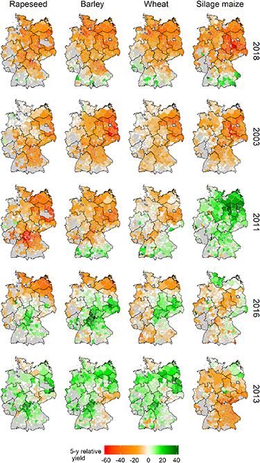
Figure 2. Relative yields (%) at NUTS3 level in statistical records for years (2018, 2003, 2011, 2016, and 2013) associated with widespread yield failure, ordered from worst to 5th worst. These observed relative yields are with respect to the Olympic average yield over the preceding 5 years for each respective NUTS3 unit. Only NUTS3 accounting for at least 0.1% of national production area of the respective crop are included in this figure.
Download figure:
Standard image High-resolution image3.3. Predicting crop yield failures
Visually, it is evident by inspecting the SVM curves that climatic variables explain more yield failures than captured by the set of processes simulated by the process-based model, with the discrepancy being largest for rapeseed and barley (figure 3). This result is irrespective of threshold selected for yield failure (Fig. S3). This is also seen in the summary Area Under the ROC curve (AUC) values (table 1). Drought stress seems to be the main process considered in the process model responsible for correct prediction of yield failures. Heat stress appears as key to capturing some failures in wheat, whereas it was less informative than variation in growing season duration for rapeseed, barley and maize. The reduced skill of the SVM in predicting yield failure in the case of maize and winter wheat may be related to the importance of considering sub-monthly processes such as heat stress or severe rain storms, the former being not strongly correlated with monthly average daily maximum temperature, particularly for maize (table S3).
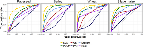
Figure 3. ROC curves to depicting the prediction accuracy of the relative yields in each of support vector machine (SVM, yellow), process-based crop model (PBCM, green) and its simulated processes: growing season duration (GS, red), intercepted photosynthetically active radiation (PAR, black), heat (purple) and the severity of drought (light blue) in classifying yield failures at the 20% loss level. Results are shown here for winter barley, silage maize, rapeseed and winter wheat across Germany for the period between 1998 and 2018.
Download figure:
Standard image High-resolution imageTable 1. Area under the ROC curve (AUC) FOR each predictor variable (support vector machine, SVM; process-based crop model, PBCM; simulated intercepted photosynthetically active radiation, PAR; simulated growing season duration, GS; drought stress, Drought; or heat stress, Heat) in classifying yield failures at the 20% loss level (20% losses relative to previous 5 year Olympic average) for winter barley, silage maize, rapeseed and winter wheat across Germany in the period 1998 to 2018.
| AUC | ||||
|---|---|---|---|---|
| Indicator | Rapeseed | Barley | Wheat | Silage maize |
| SVM | 0.89 | 0.96 | 0.92 | 0.90 |
| PBCM | 0.75 | 0.88 | 0.83 | 0.88 |
| PAR | 0.49 | 0.43 | 0.42 | 0.56 |
| GS | 0.69 | 0.68 | 0.68 | 0.72 |
| Drought | 0.69 | 0.81 | 0.83 | 0.83 |
| Heat | 0.62 | 0.55 | 0.71 | 0.67 |
3.4. Drivers of spatial patterns in yield failures across crops
To understand which processes and drivers explained spatial patterns in observed yield failures, two separate Type I ANOVAs of the spatial variation of relative yields were performed for the 5 worst years for each crop. In the first ANOVA (figure 4(a)), we first controlled for the SVM, with the remaining variation successively controlled for by the processes captured in the crop model, finally controlling for any remaining variation with state fixed effects. This analysis indicated that spatial variation in monthly weather variables could usually explain 50%–80% of the spatial variation in the relative yield changes in these extreme years, particularly for the winter cereals. With few exceptions, factors considered by the process-based model explained little additional variation.

Figure 4. ANOVA (Type I sum of squares) to show the amount of variation in relative yield levels across Germany in extreme years explained by variation in (a) monthly climate means as captured by the SVM (purple) with remaining variation captured by factors simulated by the process-based model: intercepted photosynthetically active radiation (yellow), growing season duration (dark blue), drought stress (green blue), heat stress (light blue), state fixed effects (lime green). Residual variation is shown as teal. Panel (b) indicates the amount of variation in relative yield levels across Germany in extreme years explained first by factors simulated by the process-based model (colors as in panel a), and the remaining unexplained variation explained by the SVM and state fixed effects. In both panels, the order factors were controlled for is indicated by the order in the legend (bottom factor controlled for first, top factor controlled for last). Results are presented for five most extreme years for each crop with years are ordered from worst to 5th worst.
Download figure:
Standard image High-resolution image
While the first analysis indicated that monthly climate variation captured by the SVM was important to describe a large proportion of the observed yield variation in bad years, it cannot directly indicate which climatic factors are most important, nor which underlying drivers or crop processes are responsible for the observed patterns. As a first step towards understanding this, we conducted a second Type I ANOVA, with a new order to control for the explanatory factors. We started with factors explained by the process-based model (in order as: intercepted photosynthetically active radiation; growing season duration; drought stress; and heat stress), then allowed the SVM followed by the state fixed effects to capture remaining variation (figure 4(b)). Our results indicate that the combination of factors that described the spatial yield variation varied between crops and years, which themselves varied in the underlying severity of yield failures and spatial patterns (figure 2). Interestingly, variation in intercepted radiation was often important to capture why yield failures are greater in some regions than others in extreme years (e.g. rapeseed in 2017, barley in 2007 or wheat in 2018), though it was generally not good at predicting yield variability (figure 1) or yield failure (figure 3) when all years were considered. Variation in drought stress and growing season duration were also important in a number of years for maize. Heat stress explained at most an additional 5% of variation. Importantly, we found that in many years (e.g. 2003, 2011, and 2016), the SVM explained large amounts of remaining variation for the winter cereals. This suggests that the process-based crop model was missing important climatic driven processes, explored further in the next section. Finally, some year and crop combinations were characterized as having large residuals, indicating that factors other than weather and soil water holding characteristics were responsible for the patterns of spatial yield variation in extreme years, which went beyond state level effects.
3.5. Underlying causes of yield failure
In what follows, we explore the cases in which climatic factors (as detected by the SVM) could explain large parts of the spatial variation that were not captured by the drivers simulated with the process-based model (figure 4(b)). In some cases, the SVM was explaining up to 60% additional variation in relative years, for example, rapeseed in 2003, or rapeseed and barley in 2011. This indicates a weather signals beyond spatial variation in radiation, growing season duration, drought or heat stress that caused some regions to experience large losses while others did not. To explore this, we considered year and crop combinations in which the SVM explained 25% of additional spatial variation in relative yields after the drivers of the process-based model were controlled for. We then selected three exemplary NUTS3 from across the country that exhibited strong regional differences: one each in Brandenburg (BB) in the East, Bavaria (BV) in the South and Lower Saxony (LS) in the Northwest. For each of the three exemplary NUTS3, we extracted the relative yield and weather records for the months and variables identified as most important by the SVM for the respective crops (underlying data in tables S4–S6). We further subset the data to consider only the crop and year combinations for these three NUTS3 in which their relative yields compared to one another could be explained by the values of their weather for the most important SVM predictors. The resulting set of crop and year combinations are presented in table 2.
Table 2. Explanation of factors driving yield losses in exemplary year and crop cases for three regions in the SVM, assessment of the PBCM performance and expert explanations2 of the reasons for the yield failures.
| Year | Crop | Regiona& rel yield | Explanation from SVM | Performance of PBCM | Expert explanation |
|---|---|---|---|---|---|
| 2003 | Rapeseed | BV (−26%) | Nov P too high in BV; Dec Tmax low in BB; May & July Tmax above opt in all, particularly BV & BB for May | Overestimated losses | Wet conditions in autumn in BB & BV delayed field operations and sowing. A cold & long winter, particularly in BB, lead to large losses in cereals, particularly barley. Frost damage was severe for BV & particularly BB, damaging winter cereals, and especially rapeseed. In LS, mildew was common until into April. Severe early summer drought was exacerbated by poor soils in BB & BV, and extreme summer heat leading to early harvestb. |
| BB (−31%) | |||||
| LS (−5%) | |||||
| Barley | BV (−18%) | June Tmin all above opt, water-holding capacity (WHC) of BV & BB 20% lower than in LS; May Tmax above optimum for all, Dec Tmin colder than opt for all; Oct Tmin warmer than optimum; Mar Tmin & P particularly cold & dry for BV & BB | Overestimated losses | ||
| BB (−39%) | |||||
| LS (−10%) | |||||
| Wheat | BV (−17%) | WHC of BV & BB 20% lower than in LS; low June P in BB, near optimum in BV & LS; April P particularly low in BV & BB; Nov P in BV & LS above optimum; Dec Tmin cold in all, especially in BB; May P low for all, esp BB & LS; Oct Tmin particularly low for BB & BV | Overestimated losses | ||
| BB (−35%) | |||||
| LS (−7%) | |||||
| 2011 | Rapeseed | BV (−11%) | Nov P above opt, particularly for BB; Dec Tmax below opt for all especially BB; Oct Tmin below optimum for BV & BB; May Tmax warm for all; Sept Tmin above opt for BB & NS | Losses underestimated | Excessive autumn rainfall delayed sowing. Long cold winter without a snow lead to widespread frost damage, particularly for rapeseed. Drought followed in the spring as well as an early May frost. July brought intense and heavy rainfall and flooding causing large harvest losses in BB & LSc. |
| BB (−33%) | |||||
| LS (−9%) | |||||
| Barley | BV (10%) | June Tmin warm for all; WHC of BV & BB 20% lower than in LS; May Tmax warmer than opt for all; Dec Tmin freezing and much below optimum for all; Oct Tmin warmer than optimum for LS; Mar Tmin colder than optimum, particularly for BB | Overestimated losses | ||
| BB (−20%) | |||||
| LS (−9%) | |||||
| 2016 | Rapeseed | BV (11%) | Nov P above opt for all, particularly LS; Dec Tmax too high for BV & BB, very high for LS; May Tmax well above opt for BB, somewhat for LS; Sept Tmin above opt for BB & LS | Losses underestimated, with losses overestimated losses in BV | Rapeseed experienced winter overkill. The growing season was characterized by frequent rains, with radiation thought to limit yields. However, in the BB rains were insufficient leading to drought. In large parts of the country, mildew was suspected to reduce rapeseed yields. Heavy rains delayed some rapeseed harvest, barley was largely unaffectedd. |
| BB (−33%) | |||||
| LS (−8%) | |||||
| Barley | BV (11%) | June Tmin above opt for all; WHC of BV & BB 20% lower than in LS; May Tmax well above opt for BB; Dec Tmin high for BB & LS; Oct Tmin warm for all; Mar Tmin above opt in BB, but also BV; Mar P below opt in BB | Satisfactory in regions with losses & the East; overestimated yields in BV | ||
| BB (−21%) | |||||
| LS (2%) | |||||
aFor Bavaria (BV), Pfaffenhofen a. d. Ilm (DE21J) weather variables are considered, for Branderburg (BB), Uckermark (DE40I), and for Lower Saxony (LS), Schaumburg (DE928). bDaten + Analysen IV/2003; https://www.deutschlandfunk.de/ernteausfaelle-absehbar.697.de.html?dram:article_id=72094; BLE Besondere Ernte- und Qualitätsermittlung (BEE) 2003. cDBV, 2011. Pressekonferenz zur Erntebilanz 2011. dDBV-Erntebericht: Unbeständige Witterung behindert den Fortgang der Erntearbeiten (https://mobil.bauernverband.de/ernte-2016-enttaeuschende-ertraege-ruecklaeufige-preise).
One of the most striking results is that each year and crop combination is characterized by different important variables. Notable is the absence of 2018 in table 2, considered an exceptional drought year for central and Northern Europe (Toreti et al 2019a), as the process-based model generally captured this well for maize and wheat and the SVM could explain little additional variation. This extreme drought year had severe yield failures across large parts of Germany and common across crops. The SVM is not expected to detect events that occur outside of the bounds of its training data. However, the other extreme years and crops presented in Table are characterized by a combination of unusual or sub-optimal conditions (Zscheischler et al 2018), that individually are not considered extremes. While it becomes quickly tedious to contrast and compare the weather variables across years and regions to explain the spatial patterns in yield failure, we illustrate a few cases in the following to highlight the unique combination of factors combining to contribute to yield failures. Considering barley in 2003, experts have attributed the near 40% lower relative yields in Brandenburg and 18% lower yields in Pfaffenhofen, Bavaria to an incredibly cold and long winter with significant frost damage for particularly Brandenburg. The severe winter conditions were followed by spring characterized by drought and heat stress. For barley, the SVM identified minimum temperature in June as the factor explaining the greatest amount of variation in yield levels and likely played an important role in determining losses in Pfaffenhofen, Bavaria, as minimum temperature was almost 6 °C higher than 9 °C, which is the optimal minimum temperature. It was similarly, 3 °C and 4 °C higher in Brandenburg and Lower Saxony. Of course, this alone is not able to explain the relative relationship between the three regions. The soils in Lower Saxony have a considerably higher water holding capacity than either other regions and this was the second most important factor for barley yields. Other important factors are maximum temperatures in May, for which Brandenburg and Bavaria were more than 4 °C and 5 °C higher than optimal as contrasted to Lower Saxony which was only 3 °C above optimal. However, the factor, which seems to have been decisive in 2003, was the December minimum temperature, which was 7 °C below optimum in Brandenburg compared to 3 °C and 4 °C below optimum for Bavaria and Lower Saxony, respectively. October minimum temperatures were above optimum in all regions. March minimum temperatures were 3 °C and almost 4 °C colder than optimum for Bavaria and Brandenburg, respectively, while they were near optimal in Lower Saxony. Interestingly, while experts characterized the autumn as wet leading to delayed sowing and field operations, autumn precipitation was only identified by the SVM (for November) as an important predictor in rapeseed and wheat, while the values were near optimal for November for Brandenburg, which experienced more severe yield failures for both crops than the other two regions, which did suffer from excessive rainfall. Nevertheless, the SVM largely successfully identified these drivers and the weather values taken in the different regions for key predictor variables supports the spatial patterns in relative yields for 2003 (table S4). Drought stress was overestimated by the process-based model, perhaps due to missing the damage due to the wet autumn in Bavaria and frost and extreme cold in Brandenburg, which would have reduced subsequent water use.
As a second illustrative example, 2011 saw 33% relative losses in Brandenburg for rapeseed as contrasted with approximately 10% losses in Bavaria and Lower Saxony. November precipitation, the most important variable in the rapeseed SVM, was higher than optimal for all regions leading to what experts explained as delayed sowing. December maximum temperature was almost 8 °C colder than optimal for Brandenburg, as compared to 5 °C and 6 °C colder for Bavaria and Lower Saxony respectively. Experts reported extensive losses due to frost that year. May maximum temperature was 3 °C to 4 °C above optimal for all regions and contributed to spring drought. However, the SVM missed the losses associated with a few frost days in early May, a month that was on average too warm. Similarly, both the SVM and process-based model missed the large reported yield losses attributed to heavy rainfall events in July.
4. Discussion and conclusions
Contrary to our initial expectation, a single answer to which process or processes drives yield failures and therefore must be considered in process-based models to improve climate risk assessments did not emerge. The most important processes varied across years, regions and crops. However, we can offer some insights on some of the climatic drivers that appeared important and that our process-based model was not able to capture: excessive rainfall, cold temperature and frost damage. While various options and approaches have been proposed to consider the impacts of extreme weather on crop yield, most crop models do not include these (Ewert et al 2015). Algorithms to account for frost damage have been proposed by Barlow et al (2015). A number of papers outline approaches to simulate heat stress (Barlow et al 2015, Eyshi Rezaei et al 2015, Gabaldón-Leal et al 2016) and this is perhaps the extreme impact that has seen the most concerted model improvement efforts in the past years (Maiorano et al 2017). Together with modeling impacts of pests and disease (Donatelli et al 2017, Savary et al 2018), capturing the various impacts of heavy rainfall is believed to be most problematic. This study demonstrated that damages from heavy rainfall, associated with delayed sowing and field operations, poor crop establishment, disease, waterlogging, flooding, and harvest losses due to lodging (van der Velde et al 2012) contribute to severe yield failures in Germany. Correct simulation of the impacts of waterlogging need to consider local scale heterogeneity in topography, soils, severe compaction below plough layer and the presence of functional drainage, which can influence ponding versus runoff and therefore soil workability, crop establishment and even nutrient leaching. Finally, correct simulation of the impacts of excessive water will require that models are improved to correctly simulate the dynamics of crop water supply and use (Kimball et al 2019).
Despite the shortcomings of the SIMPLACE-based model solution used here, our study also makes clear the need to continue to apply, albeit improved, process-based model. Indeed, the inability of the SVM to capture large losses in 2018 which is considered the worst year in the 20 year period (Toreti et al 2019a) and was here treated as independent data, illustrates the potential limitations of relying on purely data driven approaches under climate change. Climate change can be expected to bring novel weather event combinations (Zscheischler et al 2018) or extremes that have not occurred in the past. Rather, in as much as we can assume that the drivers of recent past yield failures are indicative of future yield failures, our results are a quiet affirmation of crop modelling community efforts such as AgMIP (Rosenzweig et al 2013), MACSUR (Ewert et al 2015) and Crops in silico(Marshall-Colon et al 2017) over the past decade to intercompare and improve crop models for climate impact assessment. Indeed, as the climate becomes more variable, we may have more extreme impacts, even without extreme events (Zscheischler et al 2018). The 2016 wheat yield drop in France provides an excellent example (Ben-Ari et al 2018). This supports the need for dynamic, process-based models that integrate the daily signals of various weather variables on biomass accumulation and leaf area growth, which in turn govern radiation capture, water use and yield formation. Leaf area dynamics driving cumulative radiation capture and water use are none the less difficult to simulate accurately as errors in either one may propagate over the course of the season. While water use is difficult to measure and depends on many processes (Webber et al 2016a), many efforts are now underway to improve its simulation (Kimball et al 2019). Leaf area dynamics play a central role for the effects of frost damage, determining radiation capture and early water use and for generic approaches to simulate pest damage (Savary et al 2018). Here on-going efforts to better assimilate and/or constrain leaf area with remotely sensing data should be intensified.
The current study suffered various limitations including using only monthly variables in the SVM, potentially underestimating the influence of heavy rainfall events in autumn and winter. A recent study for US maize demonstrated that losses due to heavy rainfall are equal to those due to drought (Li et al 2019). Here, losses due to excessive precipitation events in autumn for barley were not well captured by the anomaly in monthly average precipitation values (results not shown). However, in almost all other cases heavy rainfall events and average monthly precipitation are correlated at 0.49 to 0.65 in autumn months (Table S3). Correlations between number of frost events and minimum temperatures is very strong, while correlations between number of hot days and maximum temperature is not as strong. However, as mentioned above, process-based models have seen many recent efforts to improve representation of heat stress events (Gabaldón-Leal et al 2016, Maiorano et al 2017, Webber et al 2018b). Another limitation of the current study is that we have not further investigated the causes of the state fixed effects and residuals in the ANOVA. Inclusion of state fixed effects served as a very approximate means to account for spatial autocorrelation, which is present to varying degrees in the different years and crops (data not shown). These suggest that our model may have missed management information influenced by state level policies or an underlying environmental variable. Due to a lack of spatially explicit cultivar data with German-wide coverage, we have assumed the same variety over the study period and the same varietal characteristics related to vernalization and photoperiod responses across the country and in time. This likely limits our ability to correctly simulate phenology and growing season duration. Similarly, the lack of spatially explicit nitrogen fertilizer data, together with having ignored likely interactions of heavy rainfalls and nitrogen losses due to leaching, is expected to introduce systematic error into our process-based model simulations. In fact national nitrogen budgets yielded a surplus decreasing from 100 kg ha−1 a−1 in 1990 to 52 kg ha−1 a−1 in 2014 (Keppner et al 2016) and most of the rivers and aquifers suffer from excessive nitrate leaching from arable fields. Previous work at an aggregate scale over Europe suggested that simulation of interannual yield variability did not improve with consideration of nitrogen limitation (Webber et al 2015). This should be more thoroughly evaluated with field level trial data or even data derived from precision farming operations (Finger et al 2019) as well as studying if this is an aggregation effect, related to poor quality fertilizer data or other reasons. Our choice of 20% reductions in relative yields as a threshold to define a yield failure is also rather subjective at the county level. While a 30% threshold is commonly used at farm level (European Commission 2014), spatial aggregation bias, which reduces crop yield variability at higher aggregation levels, justifies the lower threshold here (Heimfarth et al 2012, Finger 2012). The choice of threshold produced only very small differences in ordering of years for each crop and did not influence selection of the four worst years across crops (data not shown). Finally, we used only a single model, not a model ensemble and another model may have performed better. However, the SIMPLACE based model solution used is fairly typical of models used in large area impact studies assessing climate change impacts in Europe (Webber et al 2018a). Despite these limitations, we believe the study has presented a novel approach to assess underlying causes of yield failures that can be extended with an ensemble and consideration of more factors, such as crop management and nutritional quality (Dalhaus et al 2020), in the SVM.
In concluding that we need to continue our efforts to improve process-based models to capture the impacts of extreme events, particularly if statistical approaches are unable to predict impacts of increasingly unique combinations of weather conditions (Ben-Ari et al 2018, Toreti et al 2019b), we must also reiterate the call for better collaboration between experimentalists and modellers to ensure models include state of the knowledge and datasets are available for the development and evaluation of model improvements (Rötter et al 2018). However, beyond the need for improved models, simulation of the risk of crop failure presents other challenges as well. Climate data which explores many realization of possible climate scenarios is needed. Perhaps more critically, modellers require protocols on how to assess risk of yield failures. While the information demands on magnitudes, likelihoods, certainties of failures will differ between breeders identifying adaptive traits and insurance companies trying to price premiums, modellers need insights on exactly what is of interest to knowledge users. Here we suggest that community-based protocol development are needed, similar to the protocols developed in projects like AgMIP (Rosenzweig et al 2013) to assess climate change impacts. Crop and climate scientists will need to formulate them together with those conducting risk assessments, many of who operate outside of academic research domains. While the obstacles to conducting robust risk assessments for cropping systems seems challenging, the demand is great and requires urgent action.
Acknowledgments
We are grateful to Susanne Schulz and Micheal Berg-Mohnicke of ZALF for their support with the cluster simulations. We thank Andreas Enders from University of Bonn and Lidia Voelker and Heike Schafer from ZALF for weather and yield data research and preparation. FE and TG acknowledge support from the German Research Foundation under Germany's Excellence Strategy, EXC-2070 – 390732324 – PhenoRob.
Footnotes
- 1
Olympic averages exclude the highest and lowest values before taking an average value.
- 2
Expert opinions were taken from press releases and newsletters of Farmer Organizations and media reports.