Robust Decadal Hydroclimate Predictions for Northern Italy Based on a Twofold Statistical Approach

 ,
,
Abstract
:1. Introduction
2. Data and Methods
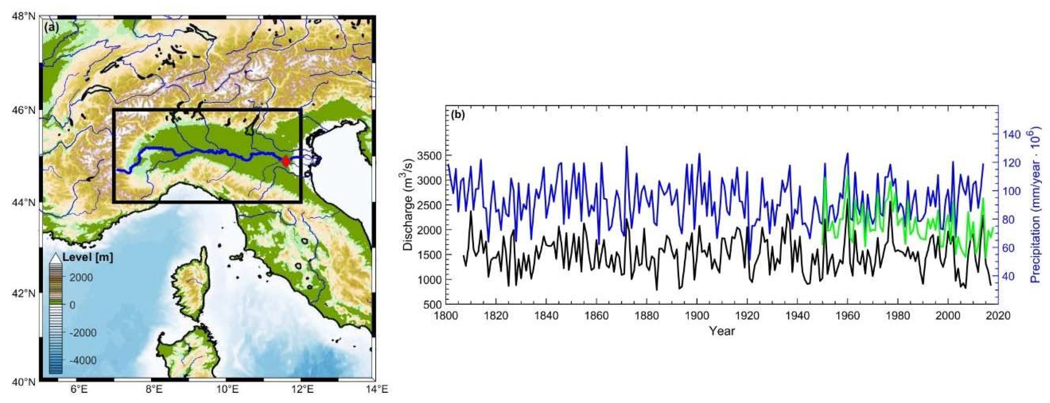
2.1. Data
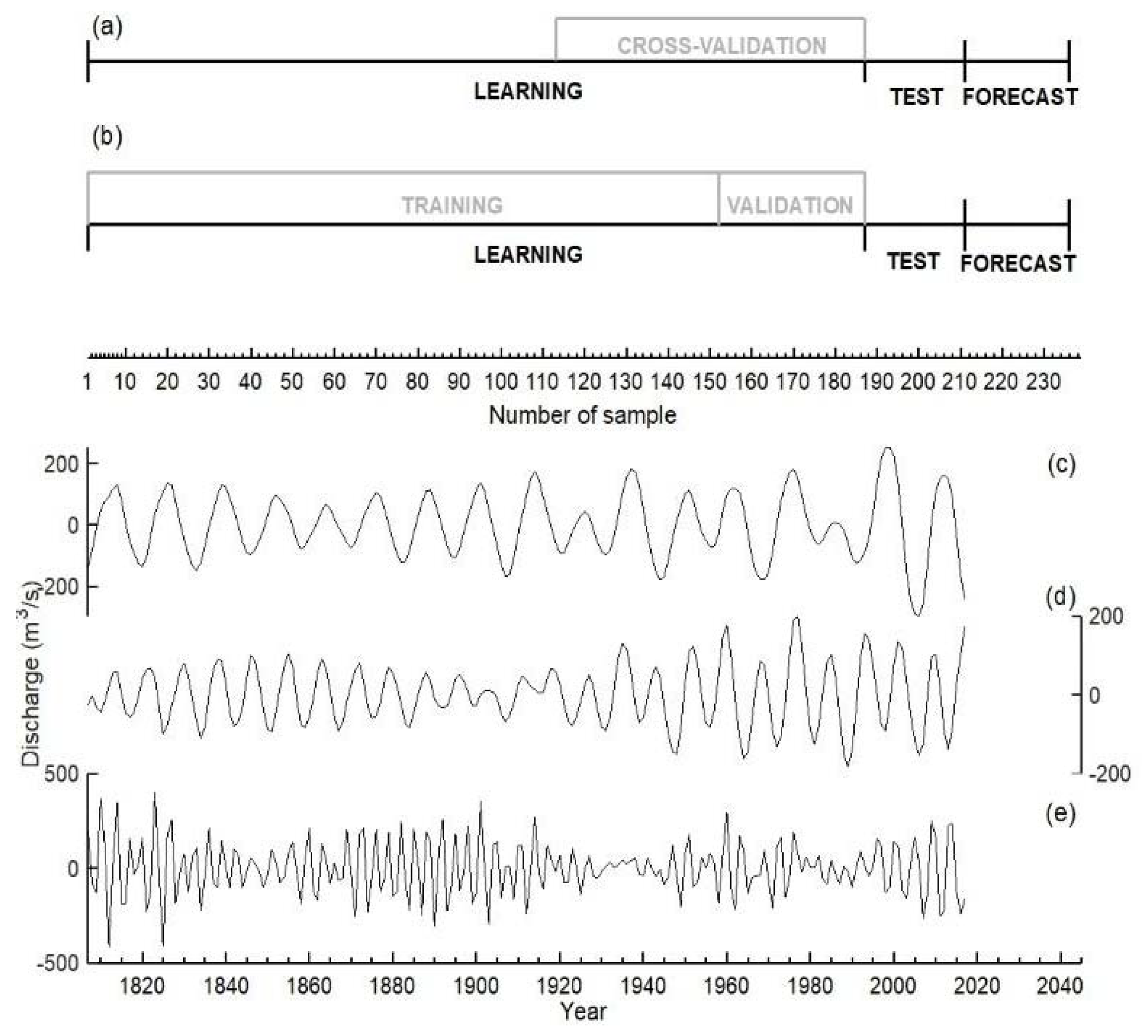
2.2. Prediction Strategy
2.2.1. Detection of Deterministic Components of the Time Series
2.2.2. AR Method
2.2.3. NN Method
2.3. Metrics for Forecast Skill and Robustness
2.4. Drought Severity Quantification
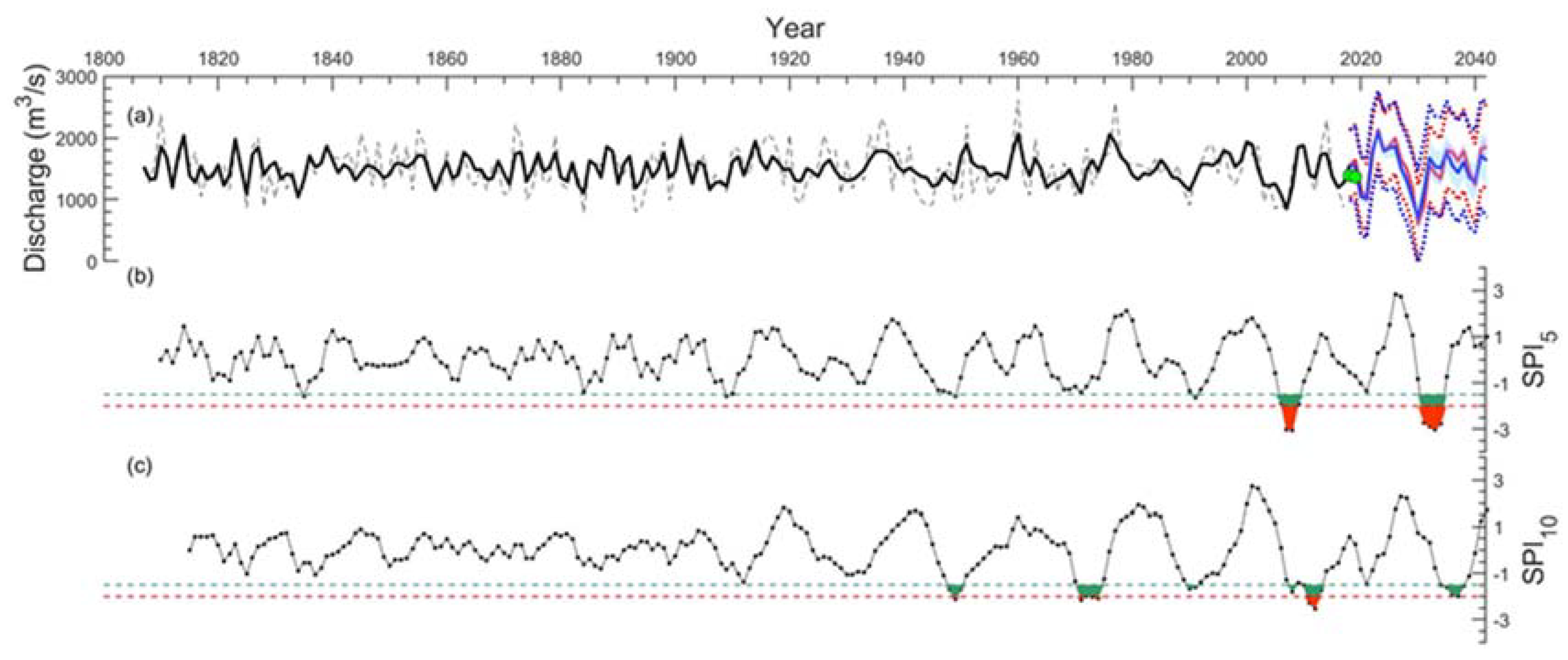
3. Results
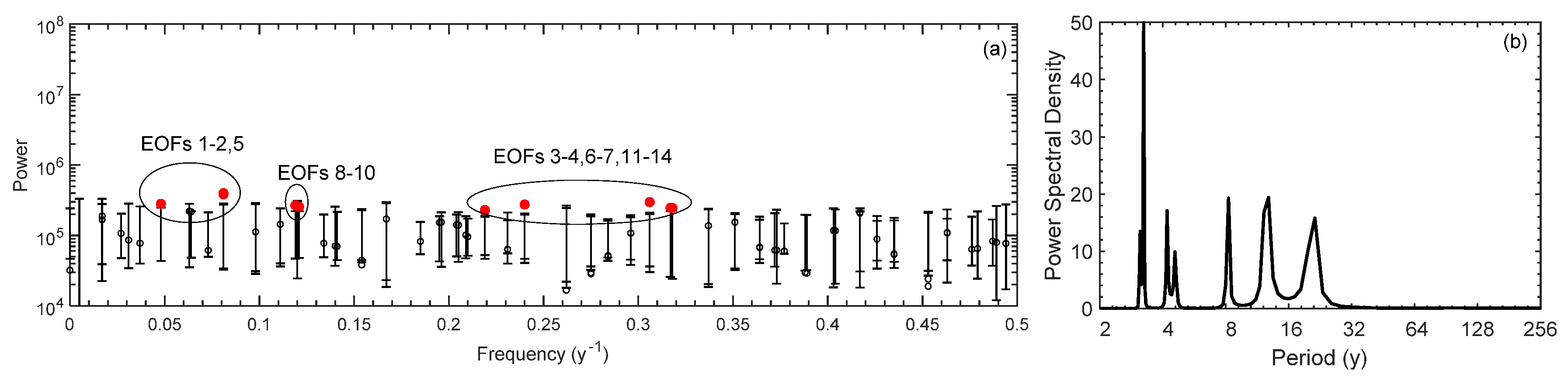
3.1. Po River Spectral Analysis
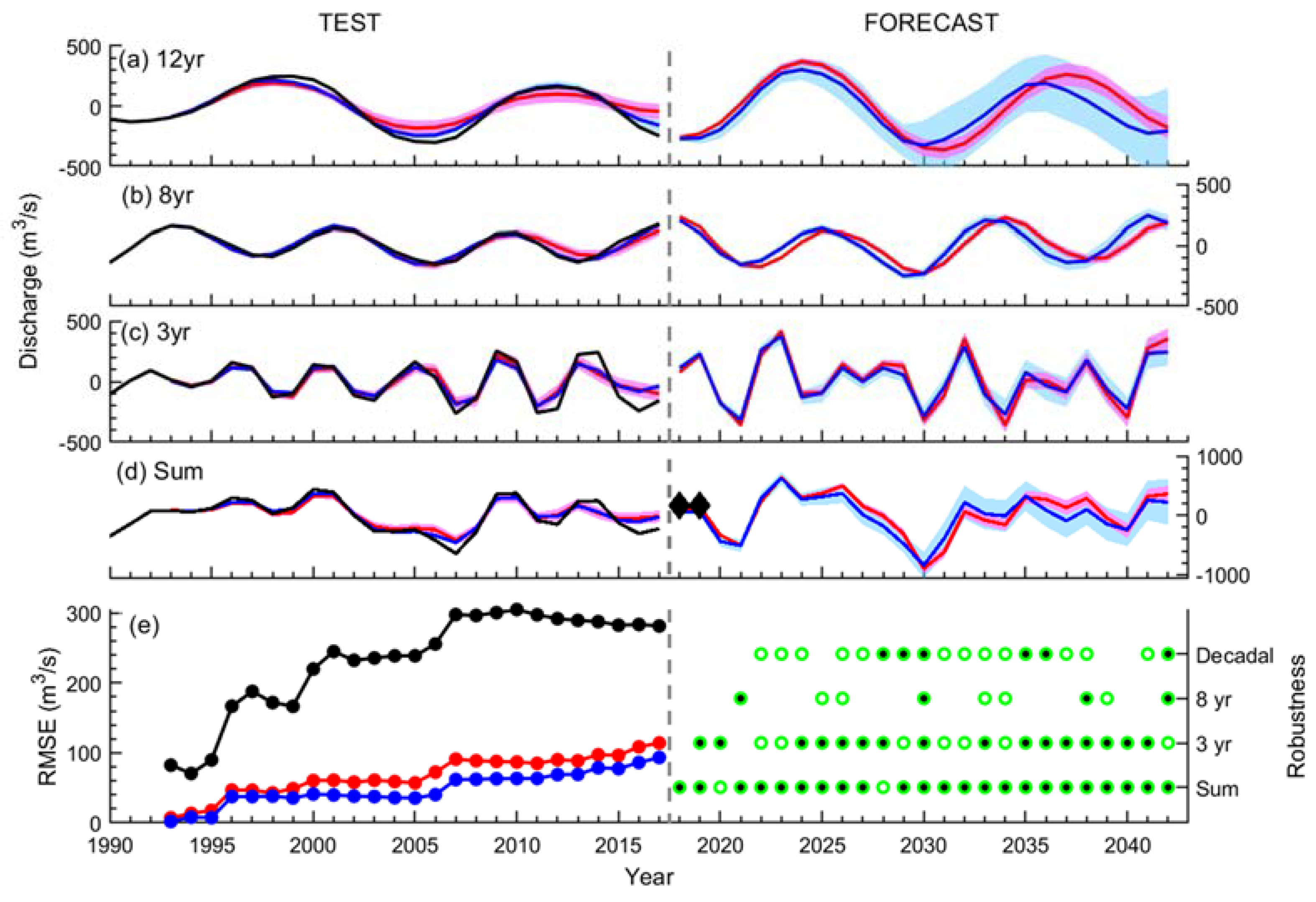
3.2. Hindcasts for the Last 25 Years
3.3. Forecast for the Next 25 Years
3.4. Evaluation of Drought Severity
4. Discussion
4.1. Rainfall vs. Runoff Processes
4.2. Methodological Aspects
4.3. Drought Severity and Attribution
4.4. Broader Climatic and Socioeconomic Implications
5. Conclusions
Author Contributions
Funding
Acknowledgments
Conflicts of Interest
Appendix A
Singular Spectrum Analysis (SSA)
Appendix B
Autoregressive Model Method
- Selection of the best order of the AR method. The AR method turns out to be most reliable and robust when the order MAR of the autoregressive model is not too large with respect to the length N of the time series, since the variance of the AR-coefficient estimates increases with the order. For this analysis, the choice of a suitable AR order is done a posteriori using goodness-of-fit criteria [35], namely the final prediction error (FPE; [36]) and the Akaike information criterion (AIC; [37]). We perform the predictions over the test section using a wide range of values of the AR model (between 1 and 60) and calculate both AIC and FPE values. The value of MAR which minimizes these indices is selected to perform the forecasts.
- Evaluation of the AR model coefficients. The values of the MAR coefficients of model are evaluated with Burg’s algorithm [38] applied to the learning section.
- Quantification of the prediction error. In order to quantify the uncertainty associated with this method, we perform 25-year predictions over different portions of this time interval (namely the cross-validation section, Figure 2a). More specifically, we repeat the procedure of the previous point varying the length of the learning section. In this way we obtain an ensemble of 25-year-predictions translated in time. By evaluating the root-mean-square-error between the predicted and original data as a function of the lead time (RMSE(l)) we obtain the uncertainty associated with the predictions. A useful scheme describing this procedure can be found in Alessio et al. [10].
Appendix C
Neural Network Method
- Partition of the learning section. While in the AR method all the data in the learning section are used to evaluate the coefficients of the model, in this case this, section is divided into two subsections: training (82% of the data in the learning section) and validation (18%). The partition can consist of continuous blocks, as shown in Figure 2b, or also in a random division of the data into the two subsets.
- Training of the network. The training set is used to compute the error gradient and update the weights and biases according to the Levenberg–Marquardt algorithm [63,64]. The validation set serves to assess the predictive skills of the NN being trained. More specifically, the error on the validation set—namely the mean squared error between predicted and observed data—is monitored during the training process and normally decreases during the initial phase of training, as does the training set error. When the network begins to overfit the data, the error on the validation set typically begins to rise. Thus, the final network weights and biases are those yielding the minimum error on the validation set. The parameter ranges of the NN architecture, namely the length I of the input vector and the numbers H1 and H2 of neurons in the hidden layers, are specifically evaluated for each component. The transfer functions used to evaluate the neuron scalar output are the sigmoid hyperbolic-tangent function for the hidden layers and the linear function for the output one.
- Prediction and quantification of the error. Each trained network is used to forecast the component in the test section, and the corresponding RMSE is calculated between predicted and observed data. Then, among all the values of I, H1 and H2, the network architecture that best reproduces the samples in the test section is chosen. The trained network is finally used for the predictions over the forecast section. Since the training process depends upon the random choice of the initial guesses for weights and biases, the procedure described above is repeated 100 times for each component, thus yielding 100 predictions. Then, the average of all the predictions in both the test and the forecasting section is evaluated, after discarding potential anomalous scenarios. Error bands associated with the predictions correspond to one standard deviation, while the standard error of the mean is used as the uncertainty associated with the average prediction.
References
- Hurrell, J.W. Decadal trends in the North Atlantic Oscillation: Regional temperatures and precipitation. Science 1995, 269, 676–678. [Google Scholar] [CrossRef] [Green Version]
- Giorgi, F. Climate change hot-spots. Geophys. Res. Lett. 2006, 33, L08707. [Google Scholar] [CrossRef]
- Gray, L.J.; Scaife, A.A.; Mitchell, D.M.; Osprey, S.; Ineson, S.; Hardiman, S.; Butchart, N.; Knight, J.; Sutton, R.; Kodera, K. A lagged response to the 11 year solar cycle in observed winter Atlantic/European weather patterns. J. Geophys. Res. Atmos. 2013, 118, 13405–13420. [Google Scholar] [CrossRef] [Green Version]
- Brunetti, M.; Maugeri, M.; Nanni, T.; Auer, I.; Böhm, R.; Schöner, W. Precipitation variability and changes in the greater Alpine region over the 1800–2003 period. J. Geophys. Res. Atmos. (1984–2012) 2006, 111. [Google Scholar] [CrossRef]
- Zanchettin, D.; Traverso, P.; Tomasino, M. Po River discharges: A preliminary analysis of a 200-year time series. Clim. Chang. 2008, 89, 411–433. [Google Scholar] [CrossRef]
- Taricco, C.; Alessio, S.; Rubinetti, S.; Zanchettin, D.; Cosoli, S.; Gačić, M.; Mancuso, S.; Rubino, A. Marine Sediments Remotely Unveil Long-Term Climatic Variability Over Northern Italy. Sci. Rep. 2015, 5. [Google Scholar] [CrossRef] [Green Version]
- Kirtman, B.; Power, S.B.; Adedoyin, A.J.; Boer, G.J.; Bojariu, R.; Camilloni, I.; Doblas-Reyes, F.; Fiore, A.M.; Kimoto, M.; Meehl, G.; et al. Near-term climate change: Projections and predictability. In Climate Change 2013 the Physical Science Basis: Working Group I Contribution to the Fifth Assessment Report of the Intergovernmental Panel on Climate Change; Cambridge University Press: Cambridge, UK, 2013; pp. 953–1028. [Google Scholar]
- Zanchettin, D. Aerosol and solar irradiance effects on decadal climate variability and predictability. Curr. Clim. Chang. Rep. 2017, 3, 150–162. [Google Scholar] [CrossRef]
- Xie, S.-P.; Deser, C.; Vecchi, G.A.; Collins, M.; Delworth, T.L.; Hall, A.; Hawkins, E.; Johnson, N.C.; Cassou, C.; Giannini, A.; et al. Towards predictive understanding of regional climate change. Nat. Clim. Chang. 2015, 5, 921–930. [Google Scholar] [CrossRef]
- Alessio, S.; Vivaldo, G.; Taricco, C.; Ghil, M. Natural variability and anthropogenic effects in a Central Mediterranean core. Clim. Past 2012, 8, 831–839. [Google Scholar] [CrossRef] [Green Version]
- Boer, G.J.; Smith, D.M.; Cassou, C.; Doblas-Reyes, F.; Danabasoglu, G.; Kirtman, B.; Kushnir, Y.; Kimoto, M.; Meehl, G.A.; Msadek, R.; et al. The decadal climate prediction project (DCPP) contribution to CMIP6. Geosci. Model. Dev. (Online) 2016, 9, 3751–3777. [Google Scholar] [CrossRef] [Green Version]
- Benestad, R.; Caron, L.-P.; Parding, K.; Iturbide, M.; Gutierrez Llorente, J.M.; Mezghani, A.; Doblas-Reyes, F.J. Using statistical downscaling to assess skill of decadal predictions. Tellus A Dyn. Meteorol. Oceanogr. 2019, 71, 1–19. [Google Scholar] [CrossRef] [Green Version]
- Po River Watershed Authority Caratteristiche del bacino del fiume Po e primo esame dell?impatto ambientale delle attività umane sulle risorse idriche. Period. Agency Rep. 2006.
- Zanchettin, D.; Rubino, A.; Traverso, P.; Tomasino, M. Impact of variations in solar activity on hydrological decadal patterns in northern Italy. J. Geophys. Res. Atmos. (1984–2012) 2008, 113, D12102. [Google Scholar] [CrossRef] [Green Version]
- Zanchettin, D.; Toniazzo, T.; Taricco, C.; Rubinetti, S.; Rubino, A.; Tartaglione, N. Atlantic origin of asynchronous European interdecadal hydroclimate variability. Sci. Rep. 2019, 9, 10998. [Google Scholar] [CrossRef] [PubMed] [Green Version]
- Tomasino, M.; Zanchettin, D.; Traverso, P. Long-range forecasts of River Po discharges based on predictable solar activity and a fuzzy neural network model. Hydrol. Sci. J. 2004, 49, 684. [Google Scholar] [CrossRef]
- Smith, D.M.; Scaife, A.A.; Eade, R.; Knight, J.R. Seasonal to decadal prediction of the winter North Atlantic Oscillation: Emerging capability and future prospects. Q. J. R. Meteorol. Soc. 2016, 142, 611–617. [Google Scholar] [CrossRef]
- Coppola, E.; Giorgi, F. An assessment of temperature and precipitation change projections over Italy from recent global and regional climate model simulations. Int. J. Climatol. A J. R. Meteorol. Soc. 2010, 30, 11–32. [Google Scholar] [CrossRef]
- Pawlowicz, R. M_Map: A Mapping Package for MATLAB. Version 1.4k. 2019. Available online: www.eoas.ubc.ca/~rich/map.html (accessed on 27 July 2019).
- Gorny, A. World Data Bank II General User GuideRep; Central Intelligence Agency: Washington, DC, USA, 1977.
- Soluri, E.; Woodson, V. World vector shoreline. Int. Hydrogr. Rev. 1990, 67, 27–35. [Google Scholar]
- Wessel, P.; Smith, W.H. A global, self-consistent, hierarchical, high-resolution shoreline database. J. Geophys. Res. 1996, 101, 8741–8743. [Google Scholar] [CrossRef] [Green Version]
- Amante, C.; Eakins, B. ETOPO1 1 Arc-minute global relief model: Procedures, data sources and analysis. NOAA Technical Memorandum NESDIS NGDC-24. Natl. Geophys. Data Cent. Noaa 2009, 10, V5C8276M. [Google Scholar]
- Auer, I.; Böhm, R.; Jurkovic, A.; Lipa, W.; Orlik, A.; Potzmann, R.; Schöner, W.; Ungersböck, M.; Matulla, C.; Briffa, K.; et al. HISTALP—historical instrumental climatological surface time series of the Greater Alpine Region. Int. J. Climatol. 2007, 27, 17–46. [Google Scholar] [CrossRef]
- Brunetti, M.; Lentini, G.; Maugeri, M.; Nanni, T.; Auer, I.; Boehm, R.; Schoener, W. Climate variability and change in the Greater Alpine Region over the last two centuries based on multi-variable analysis. Int. J. Climatol. 2009, 29, 2197–2225. [Google Scholar] [CrossRef]
- Efthymiadis, D.; Jones, P.D.; Briffa, K.R.; Auer, I.; Böhm, R.; Schöner, W.; Frei, C.; Schmidli, J. Construction of a 10-min-gridded precipitation data set for the Greater Alpine Region for 1800–2003. J. Geophys. Res. Atmos. 2006, 111, D01105. [Google Scholar] [CrossRef] [Green Version]
- Haylock, M.; Hofstra, N.; Klein Tank, A.; Klok, E.; Jones, P.; New, M. A European daily high-resolution gridded data set of surface temperature and precipitation for 1950–2006. J. Geophys. Res. Atmos. 2008, 113, D20119. [Google Scholar] [CrossRef] [Green Version]
- Taricco, C.; Ghil, M.; Alessio, S.; Vivaldo, G. Two millennia of climate variability in the Central Mediterranean. Clim. Past 2009, 5, 171–181. [Google Scholar] [CrossRef] [Green Version]
- Taricco, C.; Alessio, S.M.; Rubinetti, S.; Vivaldo, G.; Mancuso, S. A foraminiferal δ18O record covering the last 2,200 years. Sci. Data 2016, 3, 160042. [Google Scholar] [CrossRef] [Green Version]
- Penland, C.; Ghil, M.; Weickmann, K.M. Adaptive filtering and maximum entropy spectra with application to changes in atmospheric angular momentum. J. Geophys. Res. Atmos. 1991, 96, 22659–22671. [Google Scholar] [CrossRef]
- Ghil, M.; Allen, M.R.; Dettinger, M.D.; Ide, K.; Kondrashov, D.; Mann, M.E.; Robertson, A.W.; Saunders, A.; Tian, Y.; Varadi, F.; et al. Advanced Spectral Methods For Climatic Time Series. Rev. Geophys. 2002, 40, 1003–1043. [Google Scholar] [CrossRef] [Green Version]
- Ghil, M.; Taricco, C. Advanced spectral-analysis methods. In Past and Present Variability of the Solar-Terrestrial System: Measurement, Data Analysis and Theoretical Models; Castagnoli, G.C., Provenzale, A., Eds.; IOS Press: Amsterdam, The Netherlands, 1997; pp. 137–159. [Google Scholar]
- Allen, M.; Smith, L. Monte Carlo SSA: Detecting irregular oscillations in the presence of colored noise. J. Clim. 1996, 9, 3373–3404. [Google Scholar] [CrossRef]
- Groth, A.; Ghil, M. Monte Carlo singular spectrum analysis (SSA) revisited: Detecting oscillator clusters in multivariate datasets. J. Clim. 2015, 28, 7873–7893. [Google Scholar] [CrossRef] [Green Version]
- Alessio, S.M. Digital Signal Processing and Spectral Analysis for Scientists: Concepts and Applications; Springer International Publishing: Cham, Switzerland, 2015. [Google Scholar]
- Akaike, H. Statistical predictor identification. Ann. Inst. Stat. Math. 1970, 22, 203–217. [Google Scholar] [CrossRef]
- Akaike, H. A new look at the statistical model identification. IEEE Trans. Autom. Control. 1974, 19, 716–723. [Google Scholar] [CrossRef]
- Burg, J.P. Maximum entropy spectral analysis. In Proceedings of the 37th Annual International Meeting, Society of Exploration Geophysicists, Oklahoma City, OK, USA, 31 October 1967. [Google Scholar]
- Hagan, M.T.; Demuth, H.B.; Beale, M.H.; De Jesús, O. Neural Network Design; PWS publishing company: Boston, MA, USA, 1996. [Google Scholar]
- Haykin, S. Neural Networks: A Comprehensive Approach; Prentice Hall: Upper Saddle River, NJ, USA, 1999. [Google Scholar]
- Matei, D.; Pohlmann, H.; Jungclaus, J.; Müller, W.; Haak, H.; Marotzke, J. Two tales of initializing decadal climate prediction experiments with the ECHAM5/MPI-OM model. J. Clim. 2012, 25, 8502–8523. [Google Scholar] [CrossRef]
- Wu, C.; Chau, K.; Fan, C. Prediction of rainfall time series using modular artificial neural networks coupled with data-preprocessing techniques. J. Hydrol. 2010, 389, 146–167. [Google Scholar] [CrossRef] [Green Version]
- Legates, D.R.; McCabe, G.J., Jr. Evaluating the use of “goodness-of-fit” measures in hydrologic and hydroclimatic model validation. Water Resour. Res. 1999, 35, 233–241. [Google Scholar] [CrossRef]
- Nash, J.E.; Sutcliffe, J.V. River flow forecasting through conceptual models part I—A discussion of principles. J. Hydrol. 1970, 10, 282–290. [Google Scholar] [CrossRef]
- Kitanidis, P.K.; Bras, R.L. Real-time forecasting with a conceptual hydrologic model: 1. Analysis of uncertainty. Water Resour. Res. 1980, 16, 1025–1033. [Google Scholar] [CrossRef]
- McKee, T.B.; Doesken, N.J.; Kleist, J. The relationship of drought frequency and duration to time scales. In Proceedings of the 8th Conference on Applied Climatology, Boston, MA, USA, 17–22 January 1993; Volume 17, pp. 179–183. [Google Scholar]
- Orfanidis, S.J. Optimum Signal Processing: An Introduction; Collier Macmillan: New York, NY, USA, 1988. [Google Scholar]
- Musolino, D.; de Carli, A.; Massarutto, A. Evaluation of socio-economic impact of drought events: The case of Po river basin. Eur. Countrys. 2017, 9, 163–176. [Google Scholar] [CrossRef] [Green Version]
- Bueh, C.; Nakamura, H. Scandinavian pattern and its climatic impact. Q. J. R. Meteorol. Soc. 2007, 133, 2117–2131. [Google Scholar] [CrossRef]
- Krichak, S.O.; Alpert, P. Decadal trends in the east Atlantic–west Russia pattern and Mediterranean precipitation. Int. J. Climatol. 2005, 25, 183–192. [Google Scholar] [CrossRef]
- Keppenne, C.L.; Ghil, M. Adaptive filtering and prediction of noisy multivariate signals: An application to subannual variability in atmospheric angular momentum. Int. J. Bifurc. Chaos 1993, 3, 625–634. [Google Scholar] [CrossRef]
- Marques, C.; Ferreira, J.; Rocha, A.; Castanheira, J.; Melo-Gonçalves, P.; Vaz, N.; Dias, J. Singular spectrum analysis and forecasting of hydrological time series. Phys. Chem. Earth Parts A/B/C 2006, 31, 1172–1179. [Google Scholar] [CrossRef]
- Ljungqvist, F.C.; Krusic, P.J.; Sundqvist, H.S.; Zorita, E.; Brattström, G.; Frank, D. Northern Hemisphere hydroclimate variability over the past twelve centuries. Nature 2016, 532, 94–98. [Google Scholar] [CrossRef]
- Bensi, M.; Rubino, A.; Cardin, V.; Hainbucher, D.; Mancero-Mosquera, I. Structure and variability of the abyssal water masses in the Ionian Sea in the period 2003-2010. J. Geophys. Res. 2013, 118, 931–943. [Google Scholar] [CrossRef] [Green Version]
- Hainbucher, D.; Rubino, A.; Klein, B. Water mass characteristics in the deep layers of the western Ionian Basin observed during May 2003. Geophys. Res. Lett. 2006, 33, L05608. [Google Scholar] [CrossRef] [Green Version]
- Rubino, A.; Hainbucher, D. A large abrupt change in the abyssal water masses of the eastern Mediterranean. Geophys. Res. Lett. 2007, 34, L23607. [Google Scholar] [CrossRef] [Green Version]
- Bozzola, M.; Swanson, T. Policy implications of climate variability on agriculture: Water management in the Po river basin, Italy. Environ. Sci. Policy 2014, 43, 26–38. [Google Scholar] [CrossRef]
- Vautard, R.; Ghil, M. Singular spectrum analysis in nonlinear dynamics, with applications to paleoclimatic time series. Phys. D 1989, 35, 395–424. [Google Scholar] [CrossRef]
- Vautard, R.; Yiou, P.; Ghil, M. Singular-spectrum analysis: A toolkit for short, noisy chaotic signals. Phys. D 1992, 58, 95–126. [Google Scholar] [CrossRef]
- SSA-MTM Toolkit. Available online: http://research.atmos.ucla.edu/tcd/ssa/ (accessed on 14 June 2017).
- Keppenne, C.L.; Ghil, M. Adaptive filtering and prediction of the Southern Oscillation index. J. Geophys. Res. Atmos. 1992, 97, 20449–20454. [Google Scholar] [CrossRef] [Green Version]
- kSpectra Toolkit for Mac OS X! Available online: http://www.spectraworks.com/web/products.html (accessed on 6 May 2020).
- Hagan, M.T.; Menhaj, M.B. Training feedforward networks with the Marquardt algorithm. IEEE Trans. Neural Netw. 1994, 5, 989–993. [Google Scholar] [CrossRef] [PubMed]
- Rumelhart, D.; Hinton, G.; Williams, R. Learning Internal Representations by Error Propagation, Parallel Distributed Processing, Explorations in the Microstructure of Cognition, ed. DE Rumelhart and J. McClelland. Vol. 1. 1986. Biometrika 1986, 71, 599–607. [Google Scholar]


| r (p-Value) | CE | PI | |
|---|---|---|---|
| AR | 0.95 (<10−4) | 0.84 | 0.79 |
| NN | 0.96 (<10−3) | 0.89 | 0.86 |
© 2020 by the authors. Licensee MDPI, Basel, Switzerland. This article is an open access article distributed under the terms and conditions of the Creative Commons Attribution (CC BY) license (http://creativecommons.org/licenses/by/4.0/).
Share and Cite
Rubinetti, S.; Taricco, C.; Alessio, S.; Rubino, A.; Bizzarri, I.; Zanchettin, D. Robust Decadal Hydroclimate Predictions for Northern Italy Based on a Twofold Statistical Approach. Atmosphere 2020, 11, 671. https://doi.org/10.3390/atmos11060671
Rubinetti S, Taricco C, Alessio S, Rubino A, Bizzarri I, Zanchettin D. Robust Decadal Hydroclimate Predictions for Northern Italy Based on a Twofold Statistical Approach. Atmosphere. 2020; 11(6):671. https://doi.org/10.3390/atmos11060671
Chicago/Turabian StyleRubinetti, Sara, Carla Taricco, Silvia Alessio, Angelo Rubino, Ilaria Bizzarri, and Davide Zanchettin. 2020. "Robust Decadal Hydroclimate Predictions for Northern Italy Based on a Twofold Statistical Approach" Atmosphere 11, no. 6: 671. https://doi.org/10.3390/atmos11060671