Skilful interannual climate prediction from two large initialised model ensembles

The use of initialised numerical climate models to make dynamical climate predictions is now an established methodology in seasonal and, more recently, decadal forecasting. However, the intermediate timescale of 'interannual' prediction has received significantly less attention but yet has the potential to give users important advanced warning of impending climate extremes. Here we explore what climate variability is predictable beyond the seasonal prediction timescale, with a particular focus on what can be skilfully predicted for the coming year from a forecast initialised in November. To study this we take advantage of two large ensembles of initialised decadal prediction systems over the long retrospective forecast (hindcast) period 1960–2018.

The prime driver for skilful seasonal forecasts is the predictability of the coupled ocean-atmosphere El Nino Southern Oscillation (ENSO) in the tropical Pacific. ENSO is the dominant mode of intraseasonal climate variability and major events (most recently the El Nino of 2015/16) are associated with near-global climate impacts, thus providing a strong motivation for the development of global seasonal prediction systems. A particular success of seasonal prediction (from both statistical and dynamical models) has been the development of skilful forecasts of monsoon rainfall which is often strongly modulated by ENSO variability in most regions. For example, dynamical seasonal monsoon rainfall predictions have been shown to be skilful for the Indian monsoon (e.g. DelSole and Shukla 2012, Jain et al 2018), the East Asian summer monsoon (e.g. Li et al 2016), the West African Monsoon (e.g. Rodrigues et al 2014) and South American monsoon (e.g. Jones et al 2012). Skilful seasonal forecasts of monsoon rainfall in these regions can provide planning information for users in many sectors, including: agriculture, hydropower, flood/drought prevention and international aid work. If skilful forecasts of monsoon rainfall variability could made at lead times beyond that of standard seasonal forecasts then that would allow users more time to prepare and take appropriate actions.

Most seasonal forecasting focuses on the coming 3-month season with a one month lead time (forecast months 2–4), although typically these systems run out to 7 months into the future. For example, the Met Office seasonal forecast system GloSea5 (MacLachlan et al 2015) has a 7 month forecast period with weekly start dates, but a relatively short 23 year hindcast period (1993–2015). The ECMWF System 5 (Johnson et al 2019) has a longer hindcast period (1981–2015) and for each hindcast year four (of the 12 monthly) initial dates are extended out to a one year forecast period, however only 15 hindcast ensemble members are available. In contrast, the maturing field of decadal climate prediction focuses on initialising longer modes of ocean variability, such as the Atlantic Multi-decadal Variability (AMV), and on the impact of changes in external forcing from natural (e.g. solar) or anthropogenic (e.g. greenhouse gas and aerosol emissions) sources (Kushnir et al 2019). This requires longer forecast periods and lead times, such as years 2–5 or 2–9 and a longer hindcast period (starting in 1960) in order to simulate different phases of multi-decadal variability. Given the considerable computational cost, only a single annual start date is used (normally 1st November) and relatively small ensemble sizes (typically 10) are used (Boer et al 2016).

The interannual prediction timescale falls between seasonal and decadal prediction activities and has received relatively little attention to date. However, some skill is likely to come from extended range predictions of ENSO (Luo et al 2008) and from the initialisation/persistence of ocean heat content anomalies in, or just below, the upper ocean mixed layer. External forcings, such as volcanic/anthropogenic aerosol emissions, greenhouse gases and solar variability may also contribute. We use the first 16 months of prediction data from two decadal prediction systems: the UK Met Office third decadal prediction system (DePreSys3, Dunstone et al 2016) and the US Community Earth System Model Decadal Prediction Large Ensemble (DPLE, Yeager et al 2018) to investigate the skill of interannual predictions. The two systems are based on different climate models and have significantly different model resolutions and initialisation strategies (described below). However, both systems have a large 40 member ensemble and cover a long 59 year hindcast (retrospective forecast) period of 1960–2018. Note that the primary aim of this paper is to combine these two systems to create a large 80 member ensemble to best estimate the forecast skill and so assess what is predictable in the year ahead (beyond the seasonal prediction timescale), rather than provide a critical comparison of the two prediction systems themselves.

We briefly introduce the two prediction systems in section 2 and then assess their skill for global and regional annual temperature forecasts in section 3. We investigate tropical prediction skill in section 4 with a particular focus on regional monsoon rainfall prediction for the extended boreal summer (MJJAS, forecast months 7–11) and winter seasons (ONDJF, forecast months 12–16). In section 5 we examine skill for surface variables in the extratropics and conclusions are given in section 6.

The DePreSys3 system (Dunstone et al 2016) is based on the HadGEM3-GC2 coupled climate model (Williams et al 2015). The atmosphere has a horizontal resolution of approximately 60 km (and 85 vertical levels) and an ocean resolution of 0.25° (75 vertical levels). A full-field data assimilating simulation is performed where the model is nudged in the ocean, atmosphere and sea-ice components towards observations. In the ocean, temperature and salinity are nudged towards a monthly analysis created using global covariances (Smith and Murphy 2007) with a 10 day relaxation timescale. In the atmosphere, temperature and zonal and meridional winds are nudged towards the ERA40/Interim (Dee et al 2011) reanalysis with a six hourly relaxation timescale. Sea ice concentration is nudged towards monthly values from HadISST (Rayner et al 2003) with a one day relaxation timescale. Hindcasts are then started from the 1st November initial conditions of this assimilation simulation.

The DPLE system (Yeager et al 2018) is based on the CESM1.1 model using the same configuration as that used in the uninitialised CESM-Large Ensemble (CESM–LE, Kay et al 2015). The atmosphere has a horizontal resolution of approximately 110 km (and 30 vertical levels) and an ocean resolution of 1° (60 vertical levels). The ocean and sea-ice components are not initialised directly (using in-situ ocean and sea ice observations), but are taken from a separate simulation forced at the surface with historical atmospheric state and flux fields. Such forced ocean-sea ice (FOSI) simulations using CESM have been shown to capture key aspects of observed ocean and sea ice variability (Danabasoglu et al 2016). No atmospheric initialisation is performed and hence atmospheric initial conditions are taken from the corresponding years in the uninitialised CESM–LE simulations.

Both systems have time-evolving natural and anthropogenic external forcings as specified in the CMIP5 (Taylor et al 2012) protocol and this includes prior knowledge of volcanic eruptions. Both systems have hindcasts initialised every 1st November from 1959 to 2017 with a 40 member ensemble size, so giving an 80 member ensemble size when combined. For this study of interannual prediction we only consider the first 16 months of each hindcast.

We first assess the systems by examining their skill in predicting global annual temperature of the coming year (forecast months 3–14). Annual global temperature is a somewhat unusual index as it is unlikely that any individual user (e.g. an industry or sector) would be directly sensitive to its variability but yet it has significant policy importance for tracking global warming. The Paris Agreement (UNFCCC 2015) aims to limit global surface temperature rise to 'well below 2 °C above preindustrial levels and to pursue efforts to limit the temperature increase to 1.5 °C above preindustrial levels'. The warmest year so far was 2016 at +1.16 °C above preindustrial and 18 of the 19 warmest years on record have occured since the year 2000. Each December the Met Office issues a global annual temperature prediction for the coming calendar year, for example 2019 was predicted to have a central estimate of +1.10 °C (with a 5–95% confidence interval of +0.98–1.22 °C) and this forecast verified well with +1.12 °C being the observed central estimate. These operational Met Office forecasts are based on the average of the DePreSys3 dynamical forecast and a statistical method (Folland et al 2013), however here we focus solely on the DePreSys3 forecast and that of the DPLE system. Observations of global mean near surface temperature are taken as the average of HadCRUT4 (Morice et al 2012), NASA-GISS (Hansen et al 2010), and NCDC (Karl et al 2015) interpolated on to a common 2.5 × 2.5° grid as used in Smith et al (2019). To quantify skill we use the centered anomaly correlation coefficient (r) which can be regarded as a skill score relative to climatology over the hindcast period. Significance is assessed at the 95% level using a one-tailed Student's t-test.

We calculate the observed and forecast global annual temperature anomalies relative to the 1981–2010 climatological reference period and then translate values to preindustrial conditions by adding the observed difference of 0.61 °C between the periods 1981–2010 and 1850–1900 (as in Smith et al 2018). The resulting anomalies are plotted in figure 1(a) for the ensemble mean of the two systems (40 members) and their combined mean (80 members). As expected due to the strong temperature trend due to increasing greenhouse gas forcing, both DePreSys3 and DPLE systems have very high skill (r > 0.95) at predicting the rising global annual temperature over the 1960–2018 hindcast period, with the combined ensemble being nominally most skilful (r = 0.98). The ensemble means from the systems follow each other closely for most of the hindcast, although we note that the largest divergence occurs in the 1980 s where DePreSys3 appears to be biased cold and the DPLE system appears to have a warm bias. The corresponding map of global temperature skill (figure 1(b)) shows significant skill for almost all locations except for parts of the Southern Ocean and Antarctica where observations are relatively sparse and robust fingerprints of global warming are more challenging to detect. We note that whilst significant, skill is relatively low for many continental land regions (e.g. Asia).

Zoom In Zoom Out Reset image size

We subtract a linear trend (calculated over 1960–2018) from both the observations and forecast systems and then recalculate skill in predicting interannual variability (figure 1(c, d)). Global annual temperature (figure 1(c)) is still well predicted by both systems (DePreSys3: r = 0.82, DPLE: r = 0.70) with the combined ensemble again giving the nominally highest skill (r = 0.84). Both systems have considerably higher skill than that provided by a simple persistance forecast (r = 0.32). Much of the interannual variability in global annual temperature is driven by the El Nino Southern Oscillation (ENSO) mode in the tropical Pacific which we will show later is skilfully predicted out to the second year. Regional skill (figure 1(d)) is also significant in most locations apart from Central Europe, Asia and parts of North America, South America, Australia and Antarctica. Skill for ocean points is also high, except over regions of strong variability (e.g. the North Atlantic Gulf Stream extension region) and the South Atlantic/Southern Ocean. The sub-polar and tropical North Atlantic regions show particularly high skill beyond the warming trend due to strong decadal variability associated with AMV.

Seasonal forecasting has long focussed on skill driven by teleconnections to ENSO variability in the tropical Pacific (e.g. Barnston 1994). Major El Nino and La Nina events cause a significant reorganisation of the climatological Walker circulation causing the regions of atmospheric ascent and descent to shift or change amplitude. Such changes can have a direct influence on regional rainfall within the tropics (e.g. tropical Australia, South America, Africa, South Asia) but also the associated anomalous convection (and upper-level divergence) can act as a source of Rossby Waves that then propagate polewards to modify extratropical circulation (e.g. Hoskins and Karoly 1981). Predictability of ENSO has long been shown to be very high on seasonal timescales (e.g. Barnston and Ropelewski 1992), but has also been reported to extend to multi-seasonal to interannual timescales (e.g. Luo et al 2008, Dunstone et al 2016). We show the rolling (3-month) seasonal mean ENSO skill from the two systems in figure 2(a). As expected, both systems have very high skill for the seasonal forecast timescale, with DePreSys3 giving higher skill than DPLE which is likely linked to the fact that DePreSys3 initialises the atmosphere. Both systems show a sharp reduction of skill in the Spring time, consistent with the well-known 'Spring predictability barrier' (Webster and Yang 1992). However, significant skill (r ≈ 0.4–0.5) remains for both systems out to the longest one year forecast lead time.

Zoom In Zoom Out Reset image size

The combined system (green line, figure 2(a)) gives the most skilful ENSO predictions (r > 0.5) for all seasons from boreal summer (JJA) to the second winter (DJF2). There are two possible explanations for this finding, either: i) due to the combined ensmeble having double the ensemble size (80 rather than 40 members), or ii) due to the partial cancellation of individual system errors in the representation of ENSO dynamics. We explore this by examining how Nino3.4 skill changes with ensemble size (figure 2(b)) using the boreal summer (MJJAS) period as an example and a bootstrap resampling methodology (without replacement). We find that skill saturates quickly with ensemble size for this Nino3.4 index, with little further gain in skill beyond ≈10 members and hence an 80 member ensemble shows no significant improvement over a 40 member ensemble (figure 2(b), green line). Furthermore, we find that for any given ensemble size, higher skill is achieved by the combined multi-system ensemble than the individual systems (this is significant at the 95% level for all ensemble sizes). It is therefore the partial cancellation of errors between the systems that leads to the increased ENSO skill of the combined system at these long lead times (in agreement with previous studies of multi-system ENSO seasonal forecasts, e.g. Peng et al 2002).

Given the significant ENSO skill exhibited by these systems beyond the seasonal timescale, we now probe whether this translates into skilful predictions of monsoon rainfall. We focus on examining extended skill beyond the traditional seasonal forecasting timescale (the coming season or 6 months). Hence we focus on an extended boreal summer (May-September, MJJAS) period corresponding to forecast months 7–11 and an extended early boreal winter period (October-February, ONDJF) corresponding to forecast months 12–16. We use previously defined global monsoon domains (Wang et al 2011, Monerie et al 2019), selected using observed GPCC (Schneider et al 2013) grid points where the annual precipitation range (difference between May-September and November-March) exceeds 2.5 mm/day. We then split these points into seven monsoon domains: C.Am (Central America), N.Af (North Africa), S.As (South Asia), and E.As (East Asia) in the Northern Hemisphere (figure 2(c)) and S.Am (South America), S.Af (southern Africa), and N.Aus (Northern Australia) in the Southern Hemisphere (figure 2(d)). Model rainfall is regridded onto the GPCC grid resolution and then the same monsoon domains are used. We note that biases in the climatological positions of the monsoon regions in the model are not accounted for in this global overview study and hence higher skill would likely be achieved by a post-processing step that accounts for spatial shifts in the modelled monsoon domain locations.

We compute the area-averaged precipitation of each monsoon domain and calculate the skill of the systems in predicting the observed monsoon variability (figure 2(d, e) - blue bars), restricting the analysis to the summer season in each hemisphere. We note that this is a simplification of monsoon behaviour, in reality there is significantly more complexity, for example some regions experience two monsoon seasons (e.g. a winter and summer monsoon). In the boreal summer season (MJJAS, months 7–11) there is significant skill for both the Central American and East Asian monsoon domains which is present for both systems. However, the South Asian monsoon region does not show significant skill for either system. The North African monsoon (primarily the Sahel region) has skill in the DePreSys3 system, but not in the DPLE system and hence not in the combined system. This is the only monsoon region with a large disagreement in skill between the two systems and is in contrast to the skilful prediction of Sahel rainfall found in decadal predictions by the DPLE system Yeager et al (2018). Sahel interannual rainfall skill in DePreSys3 has already formed part of a previous publication (Sheen et al 2017), where ENSO variability was found to be the prime driver of high-frequency variability, whilst low-frequency changes were found to be driven by the North Atlantic SSTs and meridional shifts in the intertropical convergence zone (ITCZ). It is likely that the DPLE system may not well represent the ENSO teleconnection and/or that there are large biases in the simulated position of the DPLE North African monsoon region (but this is left for future work). Combining all four boreal summer monsoon regions, we calculate the skill in predicting the 'hemispheric' monsoon variability (right most bar in figure 2(d)). Both systems are found to skilfully predict this hemispheric metric that could be of interest to those users (e.g. aid agencies) that have global interests. In the austral summer season (ONDJF, months 12–16) significant skill is shown for the South American and Northern Australian monsoon domains, but not for the South African region. Similarly, the hemispheric average also shows significant skill. The combined skill appears to be approximately equal to the skill of the highest of the two systems but generally does not exceed it. This suggests that tropical rainfall skill is not strongly limited by ensemble size, in agreement both with other studies (e.g. Scaife et al 2019b) and that already shown for ENSO skill itself (figure 2(b)).

The skill scores calculated thus far are for all 59 years of the hindcast. However, it is possible that higher levels of skill might be present in some years. A prime candidate for such state dependent predictability is ENSO activity (DiNezio et al 2017). Given the significant ENSO skill (r ≈ 0.5) found on this interannual timescale (figure 2(a)), we test whether skill is higher when an active ENSO season is forecast. Using a threshold of ±0.5 K for the combined forecast ensemble mean signal in the Nino3.4 region we find 23 'active' years for both boreal and austral summer seasons. The calculated rainfall skill over this 23 year subset is shown by red bars in figure 2(d, e) (note that the reduced sample size is accounted for in the significance testing). All monsoon regions show a nominal improvement in skill when an active ENSO season is forecast, with most regions now approaching a skill score of r ≈ 0.5. The South Asian and East regions benefit particularly, with the former now showing significant skill.

Global skill maps for temperature, rainfall and mean sea level pressure (MSLP) are shown in figure 3(a–f). For temperature, we again focus on the forecast systems ability to predict interannual variability and so linearly detrend the observation and forecast data. We verify rainfall against the GPCC dataset over land points and the JRA55 reanalysis (Kobayashi et al 2015) rainfall over ocean points (noting that satellite derived rainfall products are not available prior to 1979). We find that JRA55 rainfall is generally in good agreement with GPCC data over land points for the hindcast period (with the notable exception of some equatorial regions, see figure S1(available at https://stacks.iop.org/ERL/15/094083/mmedia)), giving some confidence in its reproduction of rainfall over ocean points. We also verify forecast MSLP against JRA55 reanalysis data.

Zoom In Zoom Out Reset image size

Over the oceans we find significant skill for temperature (figure 3(a, b)) in most basins in boreal summer with skill reducing by boreal winter. We also find significant skill for rainfall over the tropical Pacific and Atlantic and in particular within the intertropical convergence zone (ITCZ) for both periods (figure 3(c, d)). However, regions of significant skill for extratropical temperature or rainfall over continental regions are more difficult to identify. One exception is for South-East Asia in MJJAS (see also figure S2), where a skill score of r = 0.64 (p < 0.001) is found for detrended temperature over China as a whole. This is consistent with previous results, for example Monerie et al (2018) showed interannual rainfall skill for a smaller region of North East China, using an early subset of DePreSys3 data (using only 26 of the 59 start dates used here). This study linked this skill to predictable variability in western Pacific Ocean temperatures which can trigger a Pacific-Japan pattern that can strongly impact East Asia's climate (Kosaka et al 2011).

We find further evidence for extratropical skill in the broad scale atmospheric circulation as shown by the MSLP (figure 3(e, f)). In MJJAS we find skill over eastern North America and southern South America, whilst in ONDJF we find skill over central Europe and over the Southern Ocean (likely linked to the Southern Annular Mode and the significant rainfall skill shown in this region in figure 3(d)). Whilst skill in these regions appears relatively high, the ensemble mean signal amplitude (ensemble mean standard deviation) is very low, as we show by calculating the ratio of predictable components (RPC, Eade et al 2014) at each gridpoint as follows:

$$\begin{equation*} RPC = \frac{\sigma_{sig}^{o}/\sigma_{tot}^{o}}{\sigma_{sig}^{f}/\sigma_{tot}^{f}}\approx\frac{r}{\sigma_{sig}^{f}/\sigma_{tot}^{f}} \end{equation*}$$

where σ_sig and σ_tot are the expected standard deviations of the predictable signal and the total variability, with superscripts 'o' and 'f' for the observations and forecasts respectively. For the forecasts, σ_sig and σ_tot are computed from the ensemble mean and individual members respectively. As $\sigma_{sig}^{o}/\sigma_{tot}^{o}$ cannot be readily assessed, a lower bound can be estimated from the anomaly correlation skill (r, as shown in figure 2(e, f)). An RPC ≈ 1 indicates that the model members have a similar signal-to-noise ratio to the observations, but an RPC > 1 indicates a signal-to-noise ratio that is too small in models. We find large RPC values (RPC > 2, figure 2(g, h)) for most regions of extratropical MSLP skill discussed above. These results are consistent with the high RPC found in previous analyses of the North Atlantic Oscillaion (NAO) on seasonal (Eade et al 2014, Athanasiadis et al 2017, Baker et al 2018) and decadal (Smith et al 2019) timescales and also for seasonal forecasts of the Southern Annular Mode (Seviour etal 2014). The fact that extratropical regions exhibit spuriously weak circulation signals suggests that the associated surface climate impacts (e.g. for temperature and rainfall variability) that are driven (to first order) by the large-scale surface winds (in geostrophic balance with the gradients of the MSLP field) are likely also underestimated.

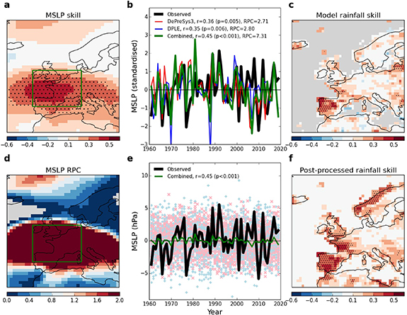
We further illustrate the weak signals and impacts on surface skill by focusing on the boreal autumn/winter (ONDJF) European signal in figure 4. Plotting MSLP skill just over the North-East Atlantic and European domain in figure 4(a), shows significant skill centred over Western Europe and less significant skill to the north of Iceland (this region is only significant at the 10% level). Both of these regions are highlighted by the map of RPC (figure 4(d)) as regions where the model has a spuriously small signal-to-noise ratio (RPC > 1). In order to assess whether these regions are associated with a mode of climate variability, we use Empirical Orthogonal Function (EOF) analysis of JRA55 reanalysis MSLP to calculate the first mode of variability over this domain. We find a dipole with centres located over Western Europe and north of Iceland (figure S3) and hence approximately co-located with the regions of MSLP skill and RPC (figure 4(a, d)). This is reminiscent of the winter (DJF) North Atlantic Oscillation (NAO) but with centres shifted further north, reflecting the northward shifted climatological position of the North Atlantic eddy-driven jet when the earlier months of October and November are also included.

Zoom In Zoom Out Reset image size

We focus on the southern node of this dipole and plot a timeseries of MSLP variability over this region (figure 4(b)) with model and observations in standardised units. We find that the combined 80 member ensemble has highly significant skill (r = 0.45, p < 0.001) and both individual systems exhibit lower but similar skill (r ≈ 0.35, p ≈ 0.005). This suggests that large model ensembles are required in order to predict the observed variations and that skill has not saturated at 40 ensemble members. The crux of this issue is illustrated in figure 4(e) which shows a version of figure 4(b) plotted in absolute units. Here the individual ensemble members are plotted for both systems, showing similar total variability to the real-world (black line) but little probabilistic skill due to the fact that each hindcast year has approximately equal numbers of members with positive and negative anomalies. If the model members were interchangable with the real-world then this would suggest low potential predictability. However, the ensemble mean (the forced predictable signal) of the 80 members correlates well with the observations but has a very small amplitude (green line, figure 4(e)) compared to that observed. This mismatch between the observations and the model systems is quantified by the large RPC (figure 4(b, d)). We note that the RPC of the combined ensemble (RPC ≈ 7) could be somewhat artificially inflated by combining two systems with slightly different modes of variability, but the fact that each system individually has an RPC ≈ 2.7 (figure 4(b)) shows that both models do indeed suffer from a small signal-to-noise ratio in this region. Another, perhaps more intuitive, way of illustrating this signal-to-noise paradox is to calculate the skill of the model predicting itself (a randomly chosen single member) and compare this to the skill of the model predicting the real world (Dunstone et al 2016). This is illustrated in figure S4, where we find very weak skill for the model predicting itself (r = 0.11) which is statistically significantly smaller than the r = 0.46 skill in predicting the observations. Furthermore, figure S4 shows how slowly the model skill for predicting real-world increases with ensemble size and that even by 80 members it is still increasing (in sharp contrast to the rapid saturation of ENSO skill with ensemble size found in figure 2(b)).

Rainfall skill over the European region is also plotted (figure 4(c)) using the raw model output for the combined ensemble. Here we find a small region of significant skill which is mainly confined to parts of the Iberian peninsular, with little skill elsewhere. However, given that we know we have a skilful, yet spuriously weak, model circulation signal we now attempt to use this to enhance the rainfall skill over this region. We follow Scaife et al (2014) and correlate the predicted ensemble mean circulation (predicted MSLP timeseries, figure 4(b, e) green line) with the observed GPCC rainfall timeseries at each gridpoint to create the skill map shown in figure 4(f). This shows a considerable improvement over the raw model rainfall skill (figure 4(c)) and we now find significant rainfall skill over a broader region of Western Europe. This includes almost all of the Iberian peninsular, western France, parts of southern England and even Norway (due to the meridional NAO-like dipole with MSLP north of Iceland).

We have investigated the skill of initialised climate predictions on the hitherto less explored interannual timescale. Using a large 80 member ensemble, along with a long 59 year hindcast, we have investigated the predictability in the coming year for surface climate variables. In general, we find an encouraging level of agreement between the two prediction systems regarding the location and strength of interannual prediction skill. This in itself is interesting given how different the two systems are in their model physics, spatial resolution and initialisation strategies.

Annual global air temperature (months 3–14) is well forecast, even beyond the warming trend. However, on the regional scale, skilful predictions over continental regions become more challenging and even average annual temperature cannot be skilfully predicted for a significant fraction of the global land regions when the warming trend is removed (figure 1(d)). Skilful predictions (r > 0.5) of seasonal ENSO variability are possible out to (and beyond) a one year lead time, in agreement with previous studies (Luo et al 2008, Dunstone et al 2016, DiNezio et al 2017). Beyond the first 6 months we find that the combined ensemble is the most skilful and we show that having a multi-system ensemble is likely more important for ENSO skill than pure ensemble size. Monsoon rainfall, key to regional agriculture and water management, shows modest but significant interannual skill in the majority of the global monsoon regions examined. Skill increases further in all regions when we consider a subset of forecast active ENSO seasons. This is promising for improved future predictions of monsoon rainfall on this potentially important interannual planning timescale.

Extratropical skill for regional surface temperature or rainfall is particularly challenging on the interannual timescale when assessed directly using model ensemble mean raw output. However, some skilful predictions are shown for atmospheric circulation in regions located near to the mid-latitude jets, particularly in the North Atlantic and Southern Ocean. Whilst the variability in many of these regions can be skilfully predicted, the amplitude of the predictable signals (the ensemble mean) are shown to be spuriously small (figure 3(g, h) and figure 4(e)). This is consistent with previous studies identifying this so-called 'signal-to-noise paradox' for extratropical circulation on seasonal to decadal timescales (Scaife and Smith 2018). Until this issue can be resolved (perhaps with considerably higher horizontal model resolution, Scaife et al 2019a), large ensembles will be needed to skilfully predict extratropical circulation (as illustrated in figure S4) and this should be considered when designing future prediction systems for interannual prediction (in common with the seasonal and decadal timescale). Related to boosting ensemble size, the use of multi-system ensembles for interannual prediction should be encouraged, as is done for seasonal predictions (e.g. the North American Multi-Model Ensemble (NMME), Kirtman et al 2014) and is now beginning for decadal predictions (Kushnir et al 2019, Smith et al 2013), when examining regional skill and producing climate services. Here we show, using the example of autumn/winter European rainfall predicted one year ahead, that these spuriously weak circulation signals can be employed to improve surface climate predictions over land.

In summary, we find encouraging signs that skilful surface climate predictions of global, tropical and extratropical regions are possible on the interannual timescale. We note that this study was limited to a single November start date and that multiple start dates would likely be of interest for interannual prediction (e.g. bi-annually or quarterly). With careful consideration of the ensemble design (e.g. using multi-model and large ensembles) useful climate services could be developed that have the potential to provide advanced warning of climate extremes.

The Met Office contribution was supported by the UK-China Research & Innovation Partnership Fund through the Met Office Climate Science for Service Partnership (CSSP) China as part of the Newton Fund. The NCAR contribution was partially supported by the U S National Oceanic and Atmospheric Administration (NOAA) Climate Program Office under Climate Variability and Predictability Program Grant NA13OAR4310138 and by the U S National Science Foundation (NSF) Collaborative Research EaSM2 Grant OCE-1243015. NCAR is a major facility sponsored by the U S NSF under Cooperative Agreement 1852977. HL Ren is sponsored by the China National Key Research and Development Program on Monitoring, Early Warning and Prevention of Major Natural Disaster (2018YFC1506004).

The data that support the findings of this study are available upon request from the authors.