


I do not know where I can find a better place than just here, to make mention of one or two other things, which to me seem important, as in printed form establishing in all respects the reasonableness of the whole story of the White Whale...
Moby-Dick; or, The Whale (Melville, Reference Melville1851).
Introduction
The 30 September 2017, Air France Flight 66 was an Airbus A380-800 (registration F-HPJE) flying from Paris, France, to Los Angeles, USA. While over southern Greenland at approximately 61.75 N, 46.85 W and 11 300 m (37 000 ft) altitude, the Number Four engine failed (Fig. 1). The failure resulted in the fan hub, fan blades and surrounding structure separating from the plane. The plane redirected to Goose Bay, Canada and landed safely. An investigation of the engine parts remaining on the plane determined that the missing fan hub, a ~220 kg piece of titanium, needed to be recovered for metallurgical examination to establish the cause of the accident. Engine remnant analysis and event modeling indicated that the fan hub likely split into two and ejected with estimated approximate initial velocities up to 133 m s−1 lateral, 244 m s−1 forward and ~43 rotations per second. Further technical details of the accident are summarized in a technical report from the Bureau d'Enquêtes et d'Analyse (BEA, 2019).
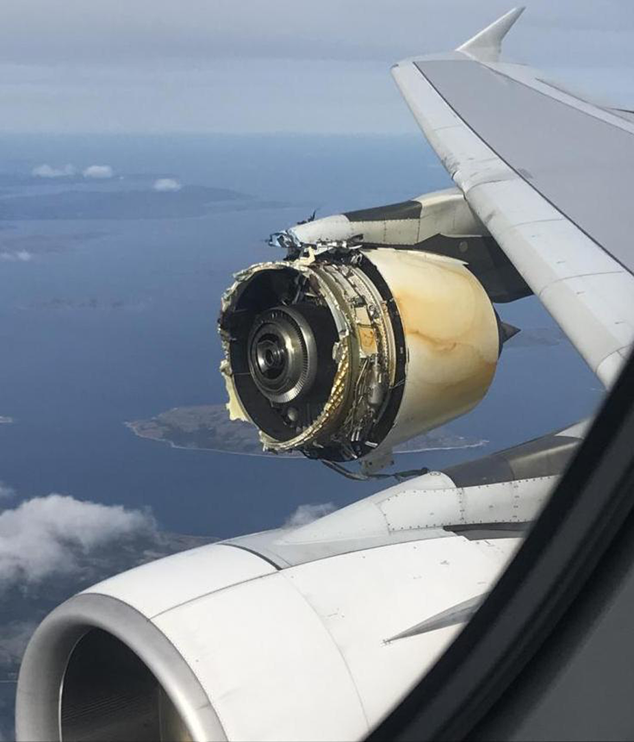
Fig. 1. The parts of engine that remained attached to the plane after the accident. Photo taken in-flight by passenger Enrique Guillen.
This is not the first accident to occur in these environments. Greenland has up to 20 planes (many from World War II (WWII)) buried within its ice sheet (Hayes, Reference Hayes1994; Boe, Reference Boe2003; Brooks, Reference Brooks2010; Talalay, Reference Talalay2020), and the frequency with which aircraft cross Greenland is likely to increase in the future. The vast Antarctic ice sheet, although more removed from global flight paths, presents a similar environment for search-and-recovery operations associated with both historical and future accidents (c.f. Alexander and Foote, Reference Alexander and Foote1998). Many aircraft have also crashed on glaciers around the world (Heggie, Reference Heggie2008; Clason and others, Reference Clason2015; Safronov, Reference Safronov2018; Compagno and others, Reference Compagno2019). Locating some of these aircraft can be challenging (e.g. Compagno and others, Reference Compagno2019 were only able to find exposed, not buried, debris). Search and recovery work at these sites is important for a variety of reasons, including environmental hazard cleanup (Clason and others, Reference Clason2015), ice velocity estimates (Ward, Reference Ward1955), ice-flow model validation (Compagno and others, Reference Compagno2019), glacial archaeology and anthropology (Dixon and others, Reference Dixon, Callanan, Hafner and Hare2014; Pilloud and others, Reference Pilloud, Megyesi, Truffer and Congram2016), repatriation of the crew and passengers (Brooks, Reference Brooks2010; Pilloud and others, Reference Pilloud, Megyesi, Truffer and Congram2016), or investigations to determine the cause of an accident to reduce the likelihood of future similar events (this project). Investigators were only able to confidently determine the cause of the failure after the fan hub fragment was recovered by this project.
The purpose of this paper is twofold, first to document the procedures and methods employed during the search campaigns, and second to serve as a guideline for similar missions to remote, crevassed, harsh-weather environments in glaciated areas. We provide an overview of the field site and environment, the search campaigns, the sensors used to first broadly and finally locally detect the part, and the tools used for the excavation.
Site and target description
Study area
The location of the search area was computed from several debris fall models from both the National Transportation Safety Board (NTSB) and Airbus and covered ~15 km2, subdivided into primary and secondary regions (Figs 2 and 3 and BEA, 2019). The search area was located to the west-north-west of where the engine failed, but ~3 km cross-track by ~5 km along-track due to uncertainty of the precise accident time (thus location), ejection speed and direction, atmospheric drag properties of the ejected pieces, atmospheric properties (wind speed and direction at various levels) and a variety of other unknown and difficult-to-model properties of the system. For example, between the 2018 and 2019 search campaigns, an adjustment of the aircraft trajectory and thus of the accident location caused the search area to shift a few hundreds of meters.

Fig. 2. Overview of field site. Fan hub fragment found to left of T1 label. T2A and T2B dots were secondary targets. Orange dots near T1 are locations of snow-covered crevasses from ground-penetrating radar (GPR) survey to T1. Airplane icon shows accident location on solid black line flight path. Dots in upper right show initial debris field. White and black dashed lines are primary and secondary search areas, respectively. Pale colored lines show GPR tracks from C4 wide-area search (right-most circles indicate C4 basecamp). C5 basecamp marked with tent icon. Bottom left shows white Greenland with circle representing the approximate location. Basemap is a contrast-enhanced Landsat image (15 m per pixel) and curved features in lower right corner are the surface depression over snow-covered crevasses.

Fig. 3. Overview of field site search area and crevasse fields. Similar to Fig. 2 except zoomed in and here basemap is an ultra-high frequency (UHF) synthetic aperture radar image from the SETHI instrument acquired during the third campaign. Approximate crevass locations are shown by light-colored streaks. Fan hub fragment location marked with X near T1. MEaSUREs 2015–2017 average velocity shown by arrows, with minimum 20 m a−1 and maximum 75 m a−1 marked at top left and bottom right, respectively.
The light-debris field was first visually identified by Air Greenland helicopter pilots sent to search the ice-sheet surface underneath where the accident occurred. The debris field was found to the north-east of the accident site due to winds blowing toward the north-east (BEA, 2019). These pilots recovered 30 pieces of light debris – fan blades and parts of the engine housing. The heavier fan hub fragments were not among this recovered debris. Because of their different aerodynamic properties and weights, the hub fragments were expected to have different fall trajectories than the light debris, and to impact to some depth below the ice-sheet's snow-covered surface where they would quickly become buried by drifting snow.
The accident occurred over the ice-sheet area that feeds Eqalorutsit Killiit Sermiat, a south-flowing glacier near the southern tip of Greenland (Bjørk and others, Reference Bjørk, Kruse and Michaelsen2015). Below the accident site (Figs 2 and 3) the ice-sheet elevation is ~1840 m above sea level (Morlighem and others, Reference Morlighem2017a, Reference Morlighem2017b), in the accumulation zone and well above the equilibrium line altitude of ~1000 m (Hermann and others, Reference Hermann2018). There is pronounced variability in local surface slope and elevation due to subglacial mountains under ~800 m of ice (Morlighem and others, Reference Morlighem2017a, Reference Morlighem2017b).
Climatology
Estimated annual surface mass balance from regional climate modeling is 0.65 m a−1 ice equivalent (Burgess and others, Reference Burgess2010), and our in situ observations showed substantial local variations. The end-of-summer 2017 until end-of-summer 2018 annual net snowfall varied from 1 to 1.5 m within the search area. The 2018–2019 net snowfall varied from 1.5 to 2.2 m. There is high spatial heterogeneity in snow properties, especially where meltwater refreezing occurred, causing ice layers and lenses throughout the firn (Fig. 4). The previous few end-of-summer layers appear as fairly uniform 5–10 cm thick ice layers, but occasional up to 5 cm thick ice lenses, spanning up to several square meters, were found between summer ice layers (Fig. 4).

Fig. 4. Density profile from April 2018 (C4). Snow pit down to 1.5 m and then nearby core from 1.5 to 12 m. Blue lines denote visible ice layers.
Prior to our field campaign, there were no ground measurements available from the area. Therefore, data from a PROMICE weather station (Programme for Monitoring of the Greenland Ice Sheet, van As and others, Reference van As and Fausto2011) were used as a first estimate of expected temperatures. From this, and to avoid summer melting and extreme cold and dark winter conditions, April and May were identified as the best months for fieldwork. During the field campaigns in April and May 2018, observed temperatures ranged from − 35 to 0 °C. May and June 2019 temperatures ranged from − 15 to + 5 °C. The dominant wind direction was east to west, ranging from calm to frequent storm events, some with steady winds of 25 m s−1 and gusts up to 32 m s−1 as a result of large low-pressure systems moving across the Atlantic Ocean just south of Greenland. During the campaigns, frequent ground-, mid- and high-level clouds and occasional snowfall and rainfall occurred at the site.
Target depth and drift
The fan hub impacted the ice sheet at an estimated 75 to 80 m s−1 according to BEA ballistic computations. Impact depth was estimated using an order-of-magnitude analysis assuming that the impactor removes a cylinder of snow with radius and mass equal to the radius and mass of the impactor, respectively, or,

where d is the estimated impact depth, m is the mass of the impactor, r is the radius of the impactor and ρ is the density of the snow. Using a mass of 100 kg (approximately half a fan hub), radius of 0.5 m and snow density of 500 kg m−3, the estimated impact depth is ~0.25 m. From this we planned for a maximum of 1 m impact depth (plus time-dependent burial) due to the large uncertainty in the non-π values, and the approximate nature of the equation.
The above estimate was tested by searching for news reports of un-exploded WWII bombs found across Europe. Typically, the bomb type and depth is mentioned in the news report. From this, radius and mass can be found (specifications for most WWII bombs can be found on Wikipedia) and the impact depth calculated from Eqn (1) can be compared to reported depth. Using this method, results from Eqn (1) have reasonable agreement with reported impact depths.
The total duration of the project was 21 months (Table I). Between remote and ground-based data acquisitions and field searches, the ice moved and the targets and search areas drifted. We used MEaSUREs velocity products from 2015 through 2017 (Joughin and others, Reference Joughin, Smith, Howat, Scambos and Moon2010, Reference Joughin, Smith, Howat and Scambos2015; Joughin, Reference Joughin2018) to estimate the minimum and maximum velocity for this drift. Ground-truth of the estimates occurred only once: A test fan hub fragment was buried in spring 2018 and re-located in spring 2019. Measurements of the two locations were done with a hand-held Global Navigation Satellite System (GNSS) device. The distance was ~60 ±5 m a−1 at ~204 degrees, within the MEaSUREs uncertainty.
Table I. Overview of field campaigns. Campaign duration is days in Greenland. Camp duration refers to nights camping on-ice. Equipment weight is the weight of equipment moved to the ice sheet for the campaign. C4 combines helicopter and Twin Otter flights

Field campaigns
This project included six field campaigns labeled C1 through C6 (Table I):
C1: The first campaign occurred 4, 8 and 11 days after the accident when Air Greenland helicopters were sent to the ground under the approximate accident location in early October 2017. The pilots found and recovered 30 pieces of debris (Fig. 2) but no fan hub fragments (BEA, 2019).
C2: The second field campaign was a single-day trip to the search area to bury a corner reflector, a Luneburg Sphere and a test fan hub fragment (one-fifth of a fan hub and only 93% scale) in March 2018 in preparation for C3.
C3: This was an airborne campaign, where synthetic aperture radar (SAR) data were acquired to identify both the test fan hub location buried during C2 (thereby empirically demonstrating sensor and algorithm capabilities), as well as detect real fan hub locations in time for C4, originally planned as the final field campaign to ground-detect (localize) and excavate the fan hub fragment(s). The SAR processing algorithms were unable to detect the test or real fan hub prior to C4.
C4: The fourth field campaign, in April and May 2018, was intended to be the final campaign. Without high-confidence radar-informed targets, we planned a ground-based campaign that included the establishment of a tent camp and extensive movement of personnel and equipment onto the ice sheet. Total duration was 4 weeks. Low-confidence targets identified in the SAR data were investigated and a wide-area grid search was done, in both cases by ground-based radar towed by snowmobile.
Post-C4: The C4 GPR was unable to reliably identify the buried test fan hub fragment, so a variety of alternate sensor options were considered for locating titanium in snow: different radar wavelengths, police sniffer dogs, RECCO detectors, micro-gravity sensors and other sensing devices. A fifth field campaign was designed following the construction of a transient electromagnetics (TEM) sensor capable of detecting a test fan hub fragment buried in snow with low false-negative and false-positive results, hereafter SnowTEM (Fig. 5). Tests were completed in Denmark at the instrument development site, and additional Greenland analog tests were done in Zermatt, Switzerland and rural Sweden (inconclusive due to remote power line interference and ground noise, respectively).

Fig. 5. A SnowTEM photograph (top) and down-looking schematic (bottom). Snowmobile with instrumentation (left), transmitter coil (center) and receiver coil (right). Dual receiver in photo is experimental setup not used during search. Photo by Thue Bording.
Meanwhile, further processing of the C3 SAR successfully identified the test fan hub fragment buried during C2, one target of interest (T1; Figs 2, 3 and 6) in the southern crevasse field, and two low-confidence, secondary targets (T2A and T2B) in the northern crevasse field (Fig. 3).
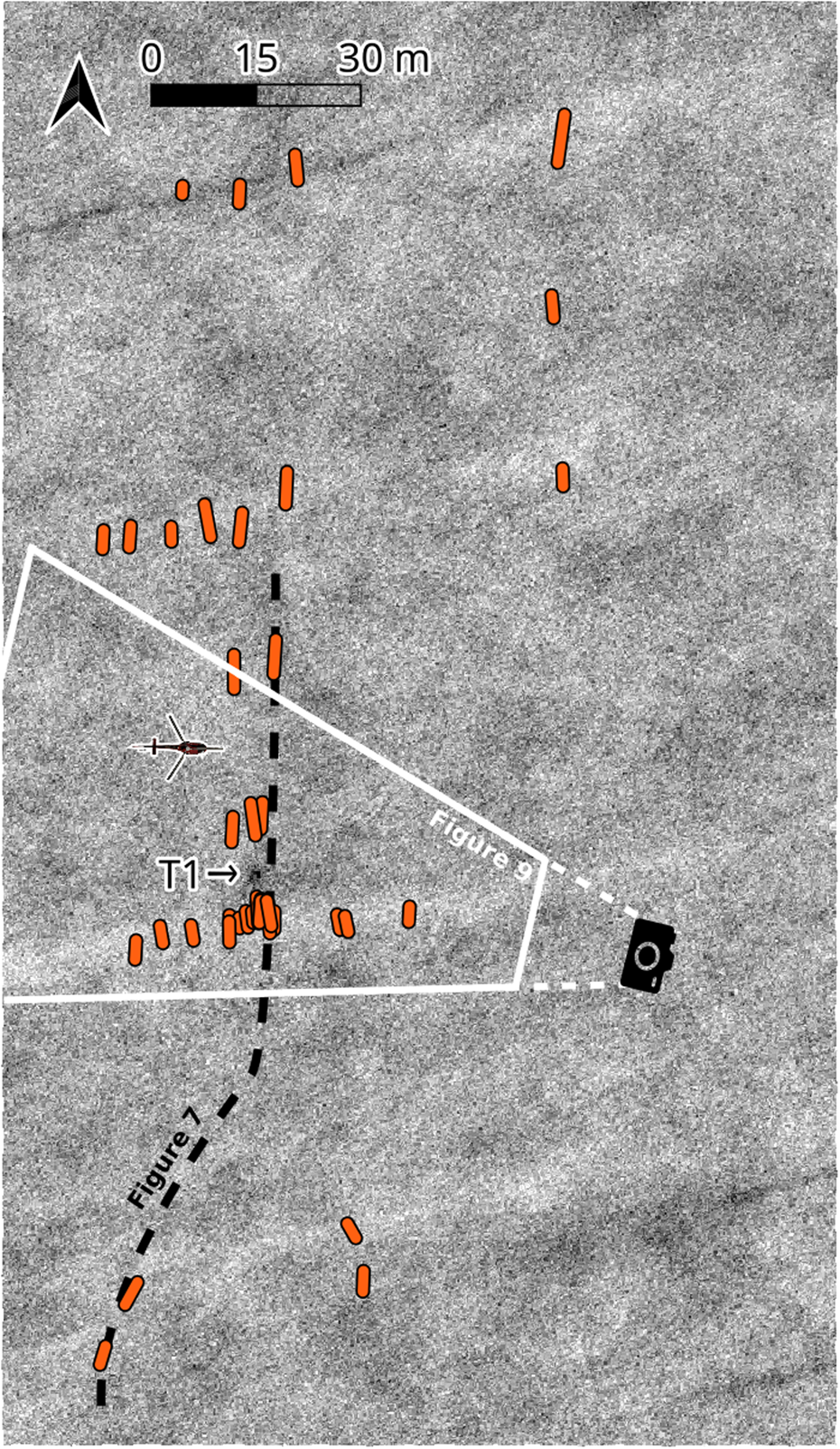
Fig. 6. Local view of Target 1 site. Basemap is 0.18 m/pixel resolution X-band composite, acquired during 2018 C3 but shifted so that target T1 lines up with location where fan hub fragment was found during 2019 C5. Dark spot near T1 arrow marks the fan hub fragment. Dark and light streaks mark crevasses, also detected during C5 FrostyBoy GPR survey and marked with orange. Black dashed line is approximate transect shown in Fig. 7. White lines and camera show approximate view and region of Fig. 9. Helicopter (credit: Rune Kraghede) added graphically at scale to show work environment (camera not to scale).

Fig. 7. Anomalous feature (in white circle and zoomed in circle) and crevasses (white boxes) from 400 MHz SIR-30 GPR towed by FrostyBoy. Near top axis, dashed box shows planned pit and work island, and tent (not to scale) marks camp island (Figs 6 and 9). On bottom axis, A and A′ refer to labels in Fig. 9. N and S refer to North and South ends of transect (see Fig. 6).
C5: The fifth field campaign was also a ground-based campaign and took place in May 2019. Although the SnowTEM had not been empirically proven to work outside of Denmark and on glacial ice, we opted to build C5 around it. The plan was to search 15 km2 (Fig. 3) over 25 days on the ice sheet by towing two SnowTEM sensors – one by snowmobile, and a second by robot in the southern crevasse field. The robot would also be used to tow a GPR, and thereby aid in the assessments of crevasse widths and snow bridge thicknesses before humans ventured into the crevasse field, should we need to excavate the fan hub or recover the robot. The C5 backup plan involved GPR point-searches of T1, T2A and T2B. Although the GPR had false-positive and false-negative issues when searching a wide area during C4, we were confident we could overcome the false-negative issue by repeat multi-directional coverage over a point target within a small search area.
C6: The final field campaign in June/July 2019 recovered the fan hub fragment. The target was located in the middle of a large field of crevasses and within ~1 m of a crevasse (Figs 6 and 7). Because of the location and the requirement that no metal (shovels) contact the fan hub, we designed the sixth campaign using fall-arrest systems, a gasoline heater to melt the fan hub out of the ice, and an electrical winch and sleds to move snow, and eventually the fan hub fragment itself, to the surface.
Remote sensing
Satellite
We used various MEaSUREs data products for estimates of ice flow velocity (Joughin and others, Reference Joughin, Smith, Howat, Scambos and Moon2010, Reference Joughin, Smith, Howat and Scambos2015; Joughin, Reference Joughin2018) and to determine strain rates; contrast-enhanced Landsat scenes and high-resolution (50 cm per pixel) optical imagery from the Pléiades satellite to check for indications of crevasses; and TerraSAR-X data to look for the buried fan hub fragment.
Airborne synthetic aperture radar: SETHI
The purpose of the airborne SAR was to detect the locations of the fan hub fragments during C3 in preparation for the C4 ground-based search. A serendipitous second benefit was insight into the extent of the crevasse field beyond what was visible in Landsat imagery (compare Figs 2 and 3).
The airborne SAR, named SETHI (Bruyant and others, Reference Bruyant2011), operated at frequencies 350 MHz (UHF-band), 1.25 GHz (L-band) and 9.6 GHz (X-band) with incidence angles of 60, 50, 45 or 40 degrees – with various incidence angles and frequency bands operated on various flights. Several frequency bands were used, as we had no a priori knowledge whether to prioritize snow/ice penetration using a lower frequency, which minimizes snow heterogeneities with respect to the wavelength, or to prioritize a higher frequency, whereby the target is large with respect to the achievable resolution and presumably more easily detectable. The antenna pattern is wider at lower frequencies, making the spatial coverage larger for lower frequencies than at higher frequencies. However, spatial resolution increases with frequency, and the higher frequency therefore resolves a larger number of pixels. A similar trade-off applies to incidence angle, whereby a higher incidence angle has a shorter underground path and lower attenuation relative to a lower incidence angle.
SETHI was installed in two pods under the wings of a Falcon 20 corporate jet. The configuration used in C3 meant that the radar could either simultaneously record left-looking L and UHF bands or only right-looking X band. Although SETHI is capable of in-flight image synthesis, the operator and console for in-flight data synthesis were removed to maximize aircraft range. Working out of Kangerlussuaq (airport code SJF) and Narsarsuaq (airport code UAK), the aircraft flew over the search area at 125 m s−1 between 2500 m and 3800 m above the ice-sheet surface, covering the site from several directions on multiple days. Precise aircraft trajectory was recorded using both an inertial navigation unit and a high accuracy GNSS receiver, allowing decimeter accuracy image geolocation.
Multiple overlapping imagery was required to increase the signal of the fan hub fragment and reduce the background noise.
Field instruments
Here, we describe the technical specifications of the instrumentation and equipment that we used throughout the field campaigns.
Ground-penetrating radar: MALÅ and GSSI
The purpose of the ice- or ground-penetrating radar was to locate the fan hub fragments during C4, and assess crevasse extent during C4 and C5.
During C4, we deployed a MALÅ RAMAC GPR with shielded antennas with center frequencies of 250 and 800 MHz. Although the 800 MHz antenna is better optimized to resolve snow and ice features up to ~20 m depth, it was actually the 250 MHz antenna, which more coarsely resolves features up to ~80 m depth, that returned a less ambiguous signal in the top ~5 m of the ice sheet when driven over the buried test fan hub fragment. The 800 MHz antenna was presumably more sensitive than the 250 MHz antenna to the spatially heterogeneous near-surface ice layers scattered across the search area. During data acquisition, every four traces were stacked to improve signal-to-noise ratio. The MALÅ GPR was towed by a snowmobile at ~2.5 m s−1. This provides ~10 cm along-track sampling with decimeter-scale depth resolution of internal ice features. The location of every GPR trace was recorded by a peripheral single-phase GNSS receiver. The horizontal resolution of GPR traces is better than ± 3 m, which was sufficient to allow returning to any targets of interest identified during post-collection GPR interpretation. This GPR configuration was towed in a tight grid pattern over a subset of the C4 search area (Fig. 2), and also used during C4 to investigate targets of interest identified during C3.
During C5, we deployed a Geophysical Survey Systems Inc. (GSSI) SIR-30 GPR with both 400 and 900 MHz shielded antennas. Similar to the experiences during C4, the lower frequency 400 MHz antenna proved superior for feature detection in the top ~20 m. The SIR-30 GPR was towed by an autonomous vehicle at ~2 m s−1, every five traces were stacked to improve the signal-to-noise ratio and provided ~16 cm along-track sampling with decimeter-scale depth resolution of internal ice features. High-accuracy differential GNSS (DGNSS) coordinates with each sample allowed us to return to locations within a few days and plant flags, marking crevasse locations. Rather than use a local base-station DGNSS setup, we used the OmniSTAR satellite-broadcast ‘correction service’.
Transient electromagnetic: SnowTEM
The purpose of the SnowTEM was to detect the fan hub fragments during C5.
TEM measurements work on the principle of inducing secondary eddy currents in surrounding materials. One method for accomplishing this is by transmitting a strong current in a coil, and rapidly turning off this current. Weak, secondary currents are induced when the primary magnetic field interacts with any other conductive object. The magnetic fields associated with these secondary currents are then measured, and any superposition of the signal can infer anomalous subsurface properties, such as buried objects (Fig. 8). The towed transient electromagnetic sensor (tTEM) has been previously designed for efficient and detailed 3D mapping of the shallow subsurface (Auken and others, Reference Auken2018). Here, we developed SnowTEM, a variant of tTEM, optimized for detection of the titanium fan hub fragment within the surrounding snow and ice. This time-domain method is in contrast to frequency-domain electromagnetic-induction systems (e.g. Haas and others, Reference Haas, Lobach, Hendricks, Rabenstein and Pfaffling2009).

Fig. 8. Plot of SnowTEM signal response showing signal strength (y-axis; dB is change in magnetic B-field, not decibel dB) vs. time (x-axis). The open symbols have opposite polarity from the closed symbols. Squares show the maximum signal from the T1 target, triangles show responses with no engine pieces, and circles show the signal from test piece. The first half (until 100 μs) of the no-engine piece signal is dominated by an internal instrument signal, and thereafter noise or couplings with opposite polarity. The three consecutive gates at 75, 100 and 132 μs were used for localization of the test piece.
The SnowTEM consists of transmitter and receiver coils mounted on sleds with a 5 m separation distance (Fig. 5). The 4 m × 4 m transmitter coil has an area of 16 m2 and four turns. The receiver coils have an area of 0.25 m2 and 160 turns. The transmitter coil is raised 0.5 m above ground to avoid sastrugi. The SnowTEM transmitter has an 800 μs on-time and repetition frequency of ~600 Hz. The SnowTEM can be towed on a 3 m lead by either snowmobile or autonomous vehicle. The main physical changes from the tTEM are the larger transmitting coil area, higher moment and more turns on the receiver coil.
The conductivity of ice and snow is too low to generate a detectable signal, leaving only the signal from the metal engine parts. The signal level from a buried object is dependent on the objects size and conductivity, and the lateral and vertical distance to the instrument coils, with signal level dropping by the distance cubed.
The SnowTEM was constructed based on numerical simulations of expected signal and noise levels, and feedback from numerous operational, tow and sensing tests done in Denmark, Switzerland and Sweden during winter 2018/2019 between C4 and C5.
Autonomous vehicles: FrostyBoy
The purpose of the FrostyBoy robot, used during C5, was threefold. (1) To tow a GPR to precisely assess crevasse locations, widths and snow bridge thicknesses, (2) to tow the SnowTEM in the crevasse field to avoid an area search by snowmobile among the crevasses, and (3) as a backup plan should the SnowTEM not work, to tow a GPR for point searches in the crevasse field.
FrostyBoy is a 100 kg uncrewed ground vehicle built to autonomously tow or carry a variety of sensors across glaciers and ice sheets. It is a derivative of Yeti and Cool Robot (Ray and others, Reference Ray, Lever, Streeter and Price2007), both of which were primarily used for GPR-based survey work in and around Antarctica's McMurdo Shear Zone (Lever and others, Reference Lever2012; Arcone and others, Reference Arcone2016).
The second purpose was never fulfilled because the drawbar pull capacity of FrostyBoy was less than the drawbar pull required to tow the SnowTEM.
Other equipment
In addition to the specialized instruments described above, the ice-sheet campaigns were also dependent on substantial reserves of more general equipment. This included helicopters, a Twin Otter and Falcon 20 fixed wing plane, two snowmobiles with sleds, multiple power generators, fuel for stoves and engines, food supplies, safety and communications gear, and all other necessary ice-sheet camping equipment.
Equipment (up to ~800 kg per sling load) was moved via Air Greenland AS-350 helicopters for C4, C5 and C6. C4 also used a Norlandair Twin Otter to move people and equipment up to ~900 kg per flight. Personnel and equipment (up to ~440 kg internal load) were moved via AS-350 for all campaigns except C3. C3 used an Aviation Défense Service Falcon 20 corporate jet.
DGNSS was used to detect precise crevasse locations from the FrostyBoy and man-hauled GPR in the crevasse field. However, due to a constantly moving ice-sheet surface, using the DGNSS coordinates to then physically flag the crevasses (Fig. 9) requires real-time (not used) or rapid post-processing for crevasse location selection and then a return to the site to plant the flags before the ice flowed far. We used the latter method.

Fig. 9. Photograph from helicopter of excavation work-site. (A and A′) Dark red graphic overlays between flags mark known crevasse locations as detected by GPR and DGNSS (also in Figs 6 and 7). Dashed lines enclose safe areas and pink marks unsafe areas defined with GPR data, the UHF basemap (Fig. 3), extensive snow probing and crevasse location uncertainty with distance from known crevasse locations. (B) Ramp out of pit. (C) Plywood used to cover pit overnight to prevent drifting snow filling. (D) Safety rope bridging crevasse between the northern (far) camp island and the southern (near) work island. (E) Sled. (F) Winch and winch platform. (G) Generator used to power winch. (H) Bamboo poles marking polar bear alarm trip-wire surrounding sleep tent. (I) Herman Nelson heater, hose and fuel barrel. (J) Helicopter landing zone. Photo by Austin Lines.
Throughout the campaigns, bamboo poles with flags were essential. They were used to mark strong GPR or SnowTEM returns when driving over targets of interest from multiple directions. Physical markers allowed us to accurately locate the subsurface point-returns of our experimental instruments by estimating precise offsets among emitters, receivers and the target(s) during multi-direction crossings. Critically, bamboo flags left erect on the ice sheet between campaigns C5 and C6 flowed with the surface, allowing us to return to precise relative positions within the crevasse field. Although DGNSS was available for our use, we found precisely geolocating a specific GPR or SnowTEM return at a specific point in time to be less useful than more coarsely locating it with bamboo flags that moved with the ice sheet, and therefore remained valid through time.
Results from remote sensing
Satellite image analysis
A high-resolution Pléiades satellite image of the region taken on 2017-10-11 (during C1) shows surface debris, a helicopter and a pilot (BEA, 2019), but no evidence of the fan hub fragment impact 11 days earlier. We were also unable to find the fan hub fragment in the TerraSAR-X data, but did not spend a significant amount of time, resources or expertise on this approach.
Crevasse detection
After the first rapid-response field campaign and before the second ground-based field campaign (i.e. between C1 and C2, See section Field Campaigns and Table I), an initial estimate of crevasse extent was done. Ice flow speed in the region is 20–75 m a−1 (Fig. 3). Strain rates in the area are < 0.02 a−1 (0.02 through 0.003 a−1). Some of these strain rates are above the critical value for crevasse formation (Colgan and others, Reference Colgan2016).
Examination of contrast-enhanced Landsat scenes in the wider area showed surface depressions indicative of snow-filled crevasses hundreds of meters long and ~30 m wide (two Landsat pixels across; Fig. 2). These large features were clearly visible in the Landsat scenes but only visible in the high-resolution (50 cm per pixel) scenes after we detected them in the Landsat scenes and knew where to look for them.
SETHI
The result of the C3 overflight was initially an ultra-high frequency (UHF) wavelength raster map (Fig. 3 basemap) showing a snow-covered crevasse field within the search area, significantly larger and with higher crevasse density than the nearby crevasse field visible in Landsat imagery (Fig. 2). The orientation of these crevasses relative to local topography suggests that these are transverse crevasses caused by tensional opening from ice flow over subglacial mountains, not shear crevasses caused by horizontal gradients in ice velocity typical of ice-stream shear margins.
Combining SAR imagery acquired from multiple elevations, directions and view angles suffers from the unknown refractive properties of the snow, ice and air (crevasse) boundaries. A known target at a known depth is needed to tune the algorithms. Initially, we identified the sphere and corner reflector in the radar imagery, but were unable to identify the test fan hub fragment or any other targets with high confidence. During the first ground campaign (C4), the SAR data were therefore primarily used for demarcating the snow-covered crevasse field (Fig. 3). However, further processing of the SAR data (between C4 and C5) successfully identified the test fan hub fragment buried during C2, one target of interest (T1, Fig. 6), and two low-confidence, secondary targets (T2A and T2B). The primary target (T1) was within the southern primary search area and 1 km into the southern crevasse field, requiring 11 crevasse crossings to reach it (Fig. 3). The two secondary targets (T2A and T2B) were just outside the search area, one in the northern crevasse field (Fig. 3). The test fan hub fragment, T2A and T2B target radar return signal strengths were ~10 decibel (dB) below the background noise from the ice, and T1 was ~8 dB below the background. To raise the signal to ~10% above background required ~100 overlapping images, collected from multiple flight tracks and multiple altitudes and sensor orientations. More details on SAR processing are contained in the Appendix.
Results from field instruments
MALÅ GPR – 2018
The C4 radar search was done with a MALÅ 250 MHz and 800 MHz GPR towed behind a snowmobile. On-site tests over the buried test fan hub fragment showed that this sensor was sub-optimal for a wide-area search. We were unable to detect the buried test fan hub fragment when driving over it with the 800 MHz antenna (false negative). The 250 MHz antenna was able to detect it depending on which direction the snowmobile was driving (i.e. orientation of the piece relative to the radar mattered). However, detection was not always successful (occasional false negatives). In addition, the signal from the test fan hub fragment was similar to the signal from the various ice lenses throughout the snow in the search area (many false positives). Finally, when we did see the test fan hub fragment it was only when directly over it, meaning dense 1 m track spacing was required, greatly reducing our possible search area given fixed time constraints.
These results were initially unexpected given that GPR has previously been used to map the extent and depth of metal and other debris within the Greenland ice sheet (Karlsson and others, Reference Karlsson2019). However, the depth, sizes and material are different. Karlsson and others (Reference Karlsson2019) observed a small town of various materials buried ~50 m deep, while we were looking for a titanium object of ~1 m3 buried ~1 m deep.
Even so, we searched the highest priority 0.5 km2 of the ~15 km2 search area at 1 m track spacing (Fig. 2), including dense repeat coverage over five possible low-confidence targets identified in the C3 SAR data. We identified anomalous signals in the C4 GPR data near most of the C3 targets, but after digging only found ice lenses – the GPR false positives also occurred in the SAR data. In total, we drove ~700 km (Fig. 2) over the course of ~15 days of driving in a 24-day field campaign. We dug six pits at potential items of interest detected in the radar data, but found only solid ice lenses at each location.
GPR probing of the crevasse field periphery by roped team members indicated crevasses with what appeared to be snow bridges < 3 m thick and with down-warping layers. We therefore did not search within the crevasse field, but determined that it was possible with other personnel and an autonomous vehicle.
In addition to the ice lenses, we were also able to identify the end-of-summer surface from 2017 (i.e. the approximate date of the fan hub impact). The May 2018 depth of the Fall 2017 surface varied from 1 to 1.5 m within the search area.
FrostyBoy and SIR-30 GPR – 2019
The SIR-30 towed by FrostyBoy was not able to detect the buried test fan hub fragment, but this may have been the result of a number of compounding factors when attempting the test (such as RF interference from FrostyBoy's communication system). In addition to not detecting the test fan hub fragment, the SIR-30 GPR also had no false positives from ice lenses. Any of a number of factors could have contributed to this difference from the MALÅ GPR, such as the difference in measurement frequency, radar systems, tow vehicles, tow speed or post-processing.
The SIR-30 400 MHz antenna was used to sound the ice sheet to depths of ~40 m and identify snow-covered crevasses (Fig. 7 and, e.g. Arcone and others, Reference Arcone2016). To estimate snow bridge thickness, we assumed a relative permittivity of 2.5, or radar speed through the firn of 1.896 × 10⁸ m s−1, slightly slower than other recent estimates of radar wave propagation through the Greenland firn (Karlsson and others, Reference Karlsson2019), which would over-estimate the snow bridge thicknesses reported below.
During the first survey to and from the T1 search area during C5, a highly reflective surface was detected at roughly 3.4 m depth (Fig. 7), ~90 m south of the T1 target location identified in the SAR data acquired during C3, a few meters outside the MEaSUREs-estimated search area. The signal was seen again at the same location during two more surveys. Given that the SIR-30 had not seen any false positives outside the crevasse field, and the strong signal was the only one of its kind seen during the different crevasse assessment surveys, this signal was deemed promising. However, based on the GPR experience from C4 we were not certain the signal came from a metallic object until a similar signal was observed with the SnowTEM.
After the object of interest was confirmed to be metallic with the SnowTEM (see below), the SIR-30 with 400 MHz antenna was repeatedly hand towed nearby to further assess crevasses around the planned excavation site (Figs 6 and 7). The data over the crevasses show that the maximum crevasse width (of those we crossed with GPR) was 10 m and had a 15 m thick bridge (ratio 1.5). The minimum crevasse width was 1 m and had a 2 m thick bridge (ratio 2). The maximum bridge thickness was 15 m on a 10 m wide crevasse (ratio 1.5). The minimum bridge thickness was 2 m on a 2 m wide crevasse (ratio 1). The maximum ratio was 3 from a 3 m wide crevasse with a 9 m thick bridge. The minimum ratio was < 1 from a 6 m wide crevasse with a 5 m thick bridge. In the Antarctic, bridge-to-thickness ratios below 1 require remediation per the US Antarctic Program (c.f. Kaluzienski and others, Reference Kaluzienski2019).
Furthermore, it was determined that the fan hub fragment could be seen when the GPR passed within 1.5 m of the fragment. Given the post-excavation-measured burial depth of 3.3–4 m, this is consistent with the GPR beam pattern and assumed radar wave propagation speed. In addition, the strong signal return on one side relative to the other was consistent in all GPR records that showed the anomalous diffraction. From knowledge gained during the excavation about the fan hub fragment's orientation in the snow, this stronger reflection was due to the different surfaces and orientation of the fan hub fragment (Fig. 7). The reason for GPR detection of the real fan hub fragment but not the test fan hub fragment may be due to their different sizes, given that their burial depths were similar.
SnowTEM
The SnowTEM functionality was first empirically verified in the field. At the conclusion of C4 we left a test fan hub fragment buried at a known location at ~2.5 m depth marked with bamboo flags taller than the 1.5 m snowfall we measured for the 2017/2018 season. These flags were buried when we returned in 2019. We were initially unable to detect the test piece while moving over it, but discovered we were able to detect it if stationary, and found it buried at 4.2 m depth. While moving, noise levels increased by 50 to 100%, due to motion-induced noise.
We then searched target T2A and T2B by driving 1–2 m spaced tracks and stopping for a few seconds every meter. The target T2A area, outside the crevasse fields, was searched twice in overlapping directions. Based on the data we confidently conclude that in the T2A area there is no engine piece with the same size or larger than the test piece, and with burial depth similar to the test piece or shallower. Target T2B, between two crevasses ~10 m apart, was searched along tracks parallel to the crevasses, to avoid driving and towing across potentially unstable snow bridges. Unfortunately, in post-processing, it was determined that the T2B target was likely not covered by the C5 T2B search area. However, the T2B target is unlikely to be an engine piece, based on its low confidence status from the strength of the C3 SAR and the C5 SnowTEM results at T2A.
Because we deemed it unreasonable to safely move the SnowTEM sensor and all other necessary equipment to T1 by snowmobile over the 11 crevasses given our access to helicopters, we created a setup that allowed helicopter transport and man-hauling. The modified SnowTEM replaced the transmitter antenna sled and frame (Fig. 5) with duct-tape and bamboo poles, and removed the sled from under the receiver coil. The modified SnowTEM worked identically to the original, albeit with some difficulty in maintaining constant geometry between transmitter and receiver coils. This modified SnowTEM fit inside a helicopter for transport to T1 and thereby avoided 11 crevasse crossings each way. We still worked over some snow-covered crevasses, but preferred to be roped and on foot (higher ground pressure) rather than on snowmobile (lower ground pressure), due both to mobility benefits and the decreased risk of injury from a manned crevasse-fall versus a snowmobile crevasse-fall, even though both were estimated as unlikely due to the snow bridge thicknesses.
Near where the SIR-30 GPR detected an anomalous feature, we recorded a signal about two orders of magnitude higher than from the buried test piece (Fig. 8), indicative of buried metal. The SnowTEM localized the fan hub fragment ~1 m north of a crevasse ~4 m wide with ~6 m bridge thickness (Figs 7 and 9). The signal was much stronger than from the test fan hub fragment due to a combination of a larger part, a shallower depth and additional non-titanium parts attached to the fan hub fragment: carbon fiber composite, aluminum, Teflon and stainless steel. The signal was strong enough that this fan hub fragment would have been detectable with the SnowTEM in motion even with the increased motion-induced noise. The fan hub fragment was clearly detectable over an area > 32 m2 – when it was within the 16 m2 transmitter coil, in a similar area between the transmitter and receiver coils, and still detectable outside this area.
Excavation
We intended to detect and excavate the fan hub fragment during the same campaign, C4 and then again C5. Due to weather delays, we were unable to excavate the fan hub fragment located during C5. The excavation required moving the necessary equipment to the site, setting up safety systems and spending an estimated 40 h of digging to excavate the fragment. We therefore left the C5 camp on-ice and planned C6 around the idea of melting the fan hub fragment out with a heater, after digging down to within a meter of the fragment. Melting would minimize metal-on-metal contact and avoid adding false flags to the investigation of the fan hub fragment after excavation.
In late June 2019, we moved the disassembled remnants of the C5 (May 2019) field camp to the T1 site ~2 km away (Fig. 3). We set up camp on an island of known solid ice 15 m wide between two crevasses, and set up our work area across one crevasse on an island of known solid ice 8 m wide where the target was located (Figs 7 and 9).
The target was within 1–1.5 m of a crevasse that was ~4 m wide with a ~6 m snow bridge (Figs 6, 7 and 9). That snow bridge width-to-thickness ratio may be safe to walk across, however, we anchored industrial fall-arrest cable-payout systems and wore construction-style (back attachment) harnesses while working at T1. This was due to concerns about digging a 4–6 m pit next to a crevasse and the possibility of large volumes of water flushing through it from surface melt, rain or melt from the heater. That water could weaken the floor and walls and the pit could collapse into the neighboring crevasse (Fig. 7).
We used ropes, chainsaws, shovels, an electric winch, sleds and a 400 000 BTU h−1 (~120 kW) Herman Nelson heater to dig down to and melt out the fan hub fragment (Fig. 9). The excavation itself was fast – only 20 h (2 days) elapsed between the beginning of digging until the part was on the surface. The top of the fan hub fragment was contacted by a shovel at an unexpectedly shallow depth of 3.3 m. The shovel contact point was marked to avoid confusing the eventual damage analysis. From the bottom of the part at ~4 m depth we estimate a ~1 m impact depth, the top of the part ~30 cm below the 30 September 2017 surface and ~3 m of subsequent snowfall. The recovered part was slightly more than half a fan hub, ~1 m3, and weighed 253.6 kg once all the snow and ice was melted off – more than the 220 kg entire fan hub because of nine attached partial fan blades.
The fan hub fragment shape is complex, the ~1 m3 is approximate, and the actual surface that impacted the snow may have been half as large, in which case Eqn (1) estimates a penetration depth of 0.64 m. Given the simplified physics assumed by that equation, it appears useful as an upper bound of impact depth for other impactors with similar properties.
We used surgical gloves while handling the fan hub to protect it from contamination from hands that had recently been in contact with a generator, winch, stove or other engines that might complicate the investigation. Contamination from other foreign material was not a concern, and the fan hub fragment was wrapped in camp mattresses, plastic tarps, plastic sleds and plywood, then slung via helicopter to the Narsarsuaq (UAK) airport. Legal chain-of-custody protocol was maintained from when the part was excavated until the part was transferred to BEA investigators.
Operational issues
Although we eventually detected and excavated the fan hub fragment, we add the following notes, some mentioned above but summarized here.
Only one of at least two fan hub fragments was found.
The test part that we used for empirically testing our instrumentation was one-fifth of a fan hub and only 93% scale. The actual part was an unknown portion of a full-scale fan hub. It ended up being just over 50%, plus parts of nine fan blades attached. Using the significantly smaller test part complicated our detection ability with both the SnowTEM and GPRs. The actual fan hub part would have been detectable with the SnowTEM in motion, and may have resulted in fewer GPR false-negatives and, from knowing what signal to look for, fewer false positives elsewhere.
The SAR overflight was unable to initially detect the test fan hub fragment, requiring large search-area campaigns instead of a targeted search campaign. Extensive algorithm development time and processing was required to generate three potential targets (see Appendix).
The SnowTEM was only able to detect the smaller, buried test fragment when stationary, and based on this we decided to use go-stop-go measurements. A full wide-area search with this approach was neither practical, nor possible within the time-frame available. This was less critical as extensive weather delays at the beginning of C5 (Table I) had changed the focus from wide-area searching to point searches.
The tow capabilities of FrostyBoy did not match the towed load of the SnowTEM, and as such could not be used to tow the SnowTEM in the crevasse field. It is possible to reduce the towed load of the SnowTEM for future applications, or use more powerful autonomous vehicles.
The RECCO sensor was discarded during the sensor search because it was unable to detect pure titanium. It is likely this low-cost hand-held or helicopter-based sensor would have detected the recovered fan hub fragment due to the variety of different attached metals.
Finally, there were extensive weather delays. Half of the campaigns had as many or more delays as scheduled flight days (Table I) due to high winds or clouds at UAK, the target site or between the two. Once we were on site, ~20 to 30% of days were unworkable due to storms, and each storm required several hours of work to deal with snow drifts and buried equipment.
Recommendations
We suggest the following workflow when searching for buried debris on ice sheets.
(1) Detection, localization and extraction campaigns should be separate because not all the information may be available until previous steps are complete. For example, if the fan hub fragment had been localized within a crevasse, or impacted and then buried to 10 m depth, the extraction effort would have changed compared to the simple extractions during C1 or the near-crevasse extraction during C6.
(2) Aerial crevasse mapping should be done before extensive ground work if possible. Based on the SAR data from C3, the crevassing in the area was substantially more extensive than first estimated (Figs 2 and 3). If such data are not available, extreme caution should be taken when first landing in an area. Given that ${\sim }50\ \percnt$
 of the region in Fig. 3 is a crevasse zone, and crevasse density may be ${\sim }20\ \percnt$, we estimate up to a ${\sim }10\ \percnt$ chance of landing on a crevasse or first-step out of a helicopter is over a crevasse, and an almost 100% chance of crossing a crevasse if moving just a few 10s of m, with possible fatal consequences (c.f May v Commonwealth of Australia, 2019). The SAR UHF-band estimated crevasse locations (Fig. 3) were only approximate, because crevasse mapping was a secondary product and the purpose of the SAR data acquisition and processing was fan hub detection. The horizontal position of an object is computed based on the range from the SAR sensor to the object and the elevation of the object. The range is measured precisely by the SAR but the elevations of the buried crevasses are unknown, and this introduces an imprecise location estimate.
(3) A thorough regional geophysical survey should be done before aerial surveys and the operational field work to assess the risk and to collect the initial data needed to interpret later geophysical data products. For example, placing DGNSS transmitters, corner reflectors and collecting snow density measurements. Sample parts should be placed near the actual site rather than at a distant analog. In this project, the sample fan hub fragment was critical to sensor validation and algorithm development – the corner reflector was too bright to be useful. If the accident site includes human remains that must be recovered (c.f. Pilloud and others, Reference Pilloud, Megyesi, Truffer and Congram2016), the search team should consider placing analog remains (i.e. pig cadavers; Schultz, Reference Schultz2008) for sensor validation and operator training.
(4) The aerial survey should use multiple resolutions, multiple sensor sand redundancy. Multiple resolutions means low (e.g. Landsat 30 m/pixel) through high (cm) resolution satellite imagery, followed by low through high resolution airborne overflights. Multiple sensors should be used because until these types of surveys become common, it is uncertain which sensors respond best to different debris shape, size, materials and surfaces. Surveys should be redundant (i.e. multiple passes with the same sensor) so that stacking and averaging algorithms can be applied (see Appendix).
(5) Once ground-based localization efforts take place, we recommend redundant, independent and autonomous sensors. Redundancy is a common field technique to avoid failures in these remote locations impacting project success – and in this project the two different GPRs behaved similarly for ‘traditional’ GPR observations of deep ice layers, but differently with respect to the ice lenses in the firn. Independent sensors are useful to cover a wide range of sensing capabilities for new target types outside the range of most glaciologists’ experience, or for common target types that are buried in a material and environment outside the range of most airplane accident investigators’ experience. Independent sensors can also cover limitations of individual sensors. For example, GPRs are a common tool operated by diverse personnel with significant polar field experience, sniffer dogs (not used here) are commonly trained to detect human remains, RECCO detectors (not used here) are lightweight and hand-held, and the SnowTEM has a large ground footprint and can be used to distinguish conductive from non-conductive material. Autonomous sensors should be used to reduce exposure to possibly high-risk work environments, increase the searchable area or decrease the search time. In the near future, heavy-lift-capable drones will likely be a new sensor platform useful for this type of field campaign.
(6) If developing new instruments, adapting existing instruments for new targets or training operators on new targets, we strongly urge future campaigns to do analog field trials of sensing instrumentation before mounting a full-scale search-and-recovery effort. When confronted with a novel search environment or sensing requirements, the best analog field site is on-site, in or adjacent to the actual search area, to avoid widely varying snow and ice conditions among different regions of the ice sheet, or the ice sheet and an alpine environment.


Summary
In September 2017, an Air France Airbus A380-800 (flight AF66, registration H-FPJE), flying from Paris to Los Angeles lost part of an engine over the Greenland Ice Sheet. An initial search area was determined by BEA using ballistic computations. The final (C5) search area, measuring ~3 km by ~5 km, was located between and within two fields of ~50 snow-covered crevasses up to ~30 m wide. With airborne SAR, this search area was reduced to three potential targets (one priority and two secondary). With the help of ground-penetrating radar, TEM and an autonomous vehicle, we confirmed that the priority target was clearly anomalous, metallic and ~1 m from a crevasse. This target was excavated using shovels, chain saws, an electric winch, sleds and a gasoline heater, by workers using fall-arrest systems. Thus, after six field campaigns, a 21-month search-and-recovery effort was successfully concluded when approximately half of a fan hub was transported from the ice sheet to Narsarsuaq, Greenland, and legal chain-of-custody was passed from a search team member to a BEA representative. The bottom of the fan hub fragment at ~4 m depth and the top at ~3.3 m depth reflect a ~1 m impact depth and ~3 m of snowfall between when impact and excavation occurred. The BEA investigation has not released the final report at the time this document was written, but an official final technical report will be published on the airplane registration F-HPJE.
The search-and-recovery of aircraft debris within snow and ice that we describe here is not unique. However, the work presented here is of general relevance for both innovative search-and-recovery operations and geophysical instrumentation. Following the failure of C4, which used conventional ground-penetrating radar instrumentation, the project was forced into a more experimental posture in C5, which used the innovative SnowTEM instrument, and introduced new sensing and integration issues. Adapting existing geophysics instrumentation for novel applications proved critical to the success of this project.
Finally, the success of this multi-phase search-and-recovery operation is a clear product of cooperation among a host of non-traditional partners, ranging from some of the world's largest aerospace and defense companies to small contractors and Ph.D. students, working in challenging conditions. The eventual success of this project reflects the combined contributions of these various actors, and highlights the value of assembling a team with extremely diverse skill sets and being willing to develop and field-test experimental technologies.
Acknowledgments
Funding for this project was provided by the Accident Investigation Board Denmark (AIB-DK), Air France, Airbus, Bureau d'Enquêtes et d'Analyse (BEA) and Engine Alliance. We are grateful for help and support from the following people and organizations. Order does not indicated level of support or level of gratitude: Arnar Ingi Gunnarsson (ICE-SAR FBSR), Anton Alsteinsson (ICE-SAR FBSR) and Tómas Eldjárn Vilhjálmsson (ICE-SAR FBSR) for their help during C6; Andreas Bergström for help during C5; Henrik Spanggård (GEUS) for logistic support during C5 and C6; Pradip Maurya (HGG), Søren Dath Møller (HGG), Lichao Liu (HGG) and Christian Lundager Nedergaard (HGG) for their help in testing and construction of the SnowTEM instrument; Zoe Courville (CRREL) for help with GPR analysis and crevasse detection; Jacky Simoud (Blue Ice Explorer) for logistic support in Narsarsuaq, and the many Greenlandic citizens who helped with last-minute equipment and supplies; Andreas Ahlstrøm (GEUS) for initiating the project; Robert Fausto (GEUS) for help with C2; Hans Jørgen Lorentzen (GEUS), Niels Jákup Korsgaard (GEUS), Jason E. Box (GEUS) and Mauro Hermann (ETHZ) for participating in C4; Lennart Brugge (RECCO) and Lars-Bertil Karlsson (RECCO) for help testing the RECCO sensors; Anjan Truffer for logistic support in Zermatt; Toke Brødsgaard, Peter Frederik Lyberth, Per Mikkelsen and many helicopter pilots from Air Greenland; many employees of Mittarfeqarfiit for help around the airport; Flemming Hougaard and the Arktisk Kommand team for providing logistic support, a hangar for the plane and a processing room during the C3 campaign in Kangerlussuaq; Norlandair; The Aviation Défense Service (AVDEF) for flying the aircraft with the L'Office National d’Études et de Recherches Aérospatiales (ONERA) sensors; The Polar Geospatial Centre for the DTM used for ONERA image synthesis (NSF OPP awards 1043681, 1559691 and 1542736); Sunny Gupta (Airbus) for helping supply Pleiades and TerraSAR-X imagery; Naor Movshovitz for suggesting the impact depth estimate equation; many additional unnamed members of the A380 F-HPJE Engine Search project at AIB-DK, Air France, Airbus, BEA, Engine Alliance, GE, GEUS, the NTSB, ONERA and other institutions. Finally, Stéphane Otin (BEA) and Anders Bjørn Kristensen (AIB-DK) for their support and encouragement throughout the project. We thank the editors and reviewers (Caroline Clason and two anonymous) for their help improving the text for publication.
Author contributions
KDM led C2, helped prepare and co-led C4, led the instrument search between C4 and C5, helped prepare and led C5 and C6, and helped write the manuscript. DVA participated in C4, C5 and C6, helped prepare C5 and C6, maintained chain-of-custody, and helped write the manuscript. AL participated in C5 and C6. TB participated in SnowTEM testing between C4 and C5, participated in C5, and helped write the manuscript. JE participated in C5 and helped write the manuscript. RK participated in C5. HC did UHF-band signal processing during C3, was responsible for signal reprocessing between C4 and C5, and helped write the manuscript. HO led the C3 signal processing and processed the L-band images. PDF initiated, organized and led C3. ORdP led the hardware group for C3 and planned the C3 data acquisition and flights. AVC built SnowTEM and participated in SnowTEM testing between C4 and C5. EA oversaw SnowTEM development. KH participated in C4 and helped prepare C5. WC assisted with planning C4, participated in C4 and helped write the manuscript. NBK initiated the field projects, helped prepare and co-led C4, helped prepare C5 and helped write the manuscript.
Conflict of interest
Financial: Authors DVA, AL and JE operate private companies that benefit financially from finding airplane engines in Greenland and other similar work. All authors and or their employers had at least some short-term financial benefits from this project.
Appendix: Synthetic aperture radar processing
The test fan hub fragment was eventually found in the radar data with a signal 10 dB below the background signal. Detecting an object with a signal amplitude equal to 10% of the background with an acceptable false-negative and -positive rate is difficult. Radar uses coherent electromagnetic waves and this coherency induces random amplitude fluctuations (speckle). These fluctuations are not strictly speaking noise – if the same measurement is done with the same flight trajectory, the signal fluctuations occur at the same positions (this property is exploited for interferometric SAR to measure precise earth motion). Real noise does exist in the observations, but in the SETHI measurement used here, the thermal noise was 3 orders of magnitude lower than the speckle. We opted not use spatial averaging to enhance the signal because this degrades the spatial resolution. The alternative is to stack independent images.
After stacking N images, the normalised standard deviation (standard deviation divided by the mean) of the fluctuations is ${\sim }1.85/\sqrt {N}$ . To detect a target with a false alarm rate below 10−9, from a search area covered by ~3.109 pixels, the target level should be higher than ~6 standard deviations of the fluctuations. For a target level of 0.1, N must be larger than 111. This is a minimum number of images, because here it would likely give three false alarms, and each false alarm equals ~15 tons of snow if digging for visual verification.
It is possible to obtain several images from one single acquisition by using different polarizations of the electromagnetic waves and by looking slightly fore and aft with respect to the antenna pointing. For the X-band, this can only raise N to ~18 from 24 images, because the four polarizations are not fully independent. We combined images from 18 acquisitions from different directions for a total of 432 images. From these 432 images, N increases to only ~200 because of polarization dependencies and incomplete overlap of the images.
Combining images from different directions has advantages and disadvantages. The target signal may depend on the direction of illumination and using acquisitions from different directions increases the chance of observing a brighter signal. But unlike images from the same acquisition, the registration (within the 20 cm of SETHI resolution) of different observations is difficult. To co-register observations, (1) sensor trajectories (i.e. flight path) must be accurate to less than ~10 cm due to lack of stationary landmarks on the ice sheet, (2) radar range must be accurate to less than ~10 cm (signal delay accuracy below 500 ps), (3) terrain surface should be accurate to ~10 cm, (4) because several days may separate acquisitions, ice drift must be known and compensated for, and (5) target depth below surface and snow/ice refraction index are only approximated, and the effect of refraction should be accurately compensated for the effective target depth. This was estimated from a known target – a cowling fragment left in the light debris field during C1.
Initial processing occurred over the full 102 000 × 110 000 pixel scene. Synthesis, registration and fusion of these 432 images required 750 h on a 120-core computer and ~40 Tb of temporary storage. A second improved processing was done over the final smaller search area – each scene was only 55 000 × 51 000 pixels.


 Open access