
Remote Sensing Measures Restoration Successes, but Canopy Heights Lag in Restoring Floodplain Vegetation

 , , and
Abstract
:
1. Introduction
2. Methods
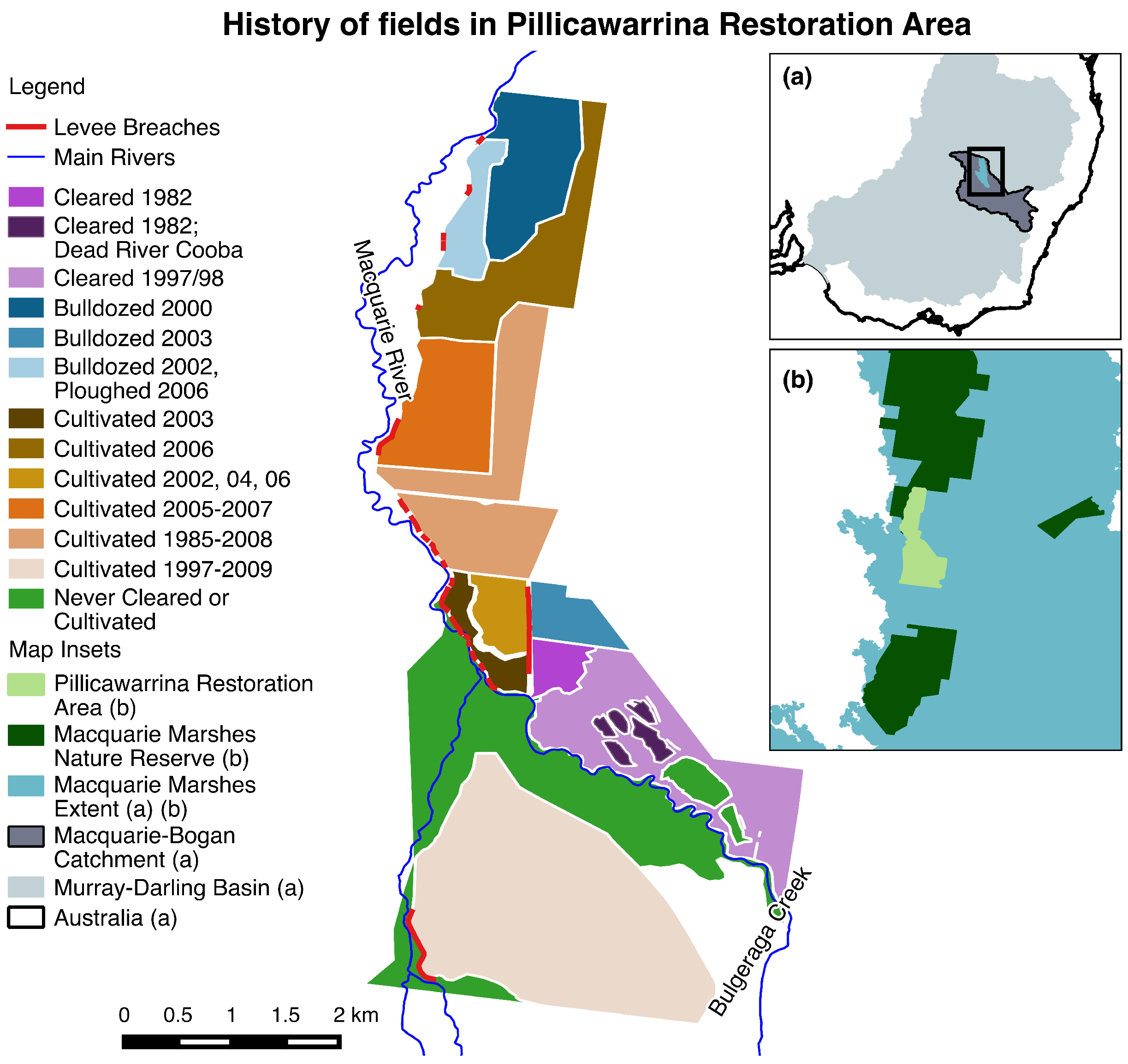
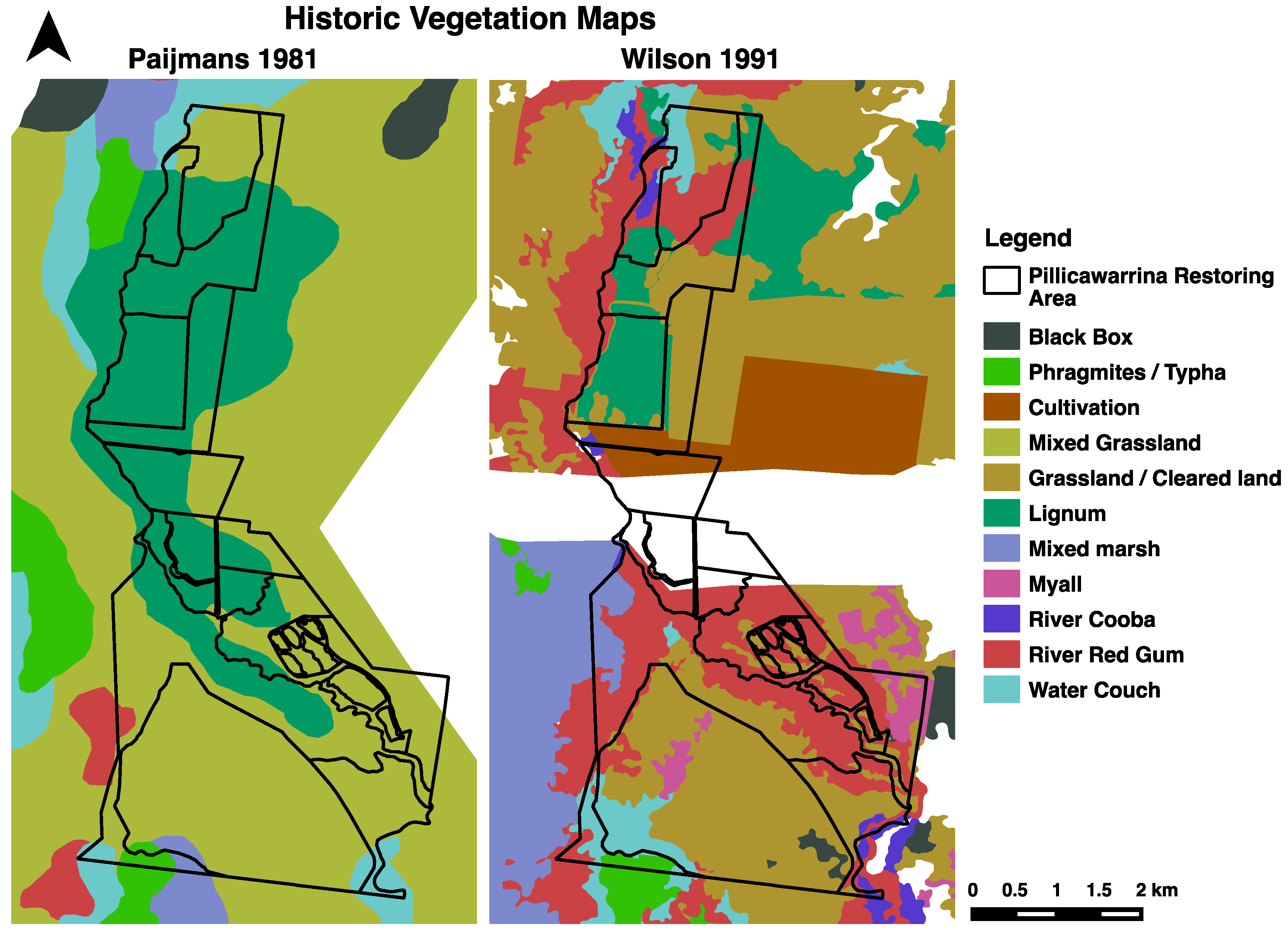
2.1. Study Site
2.2. Restoration and Floodplain Vegetation
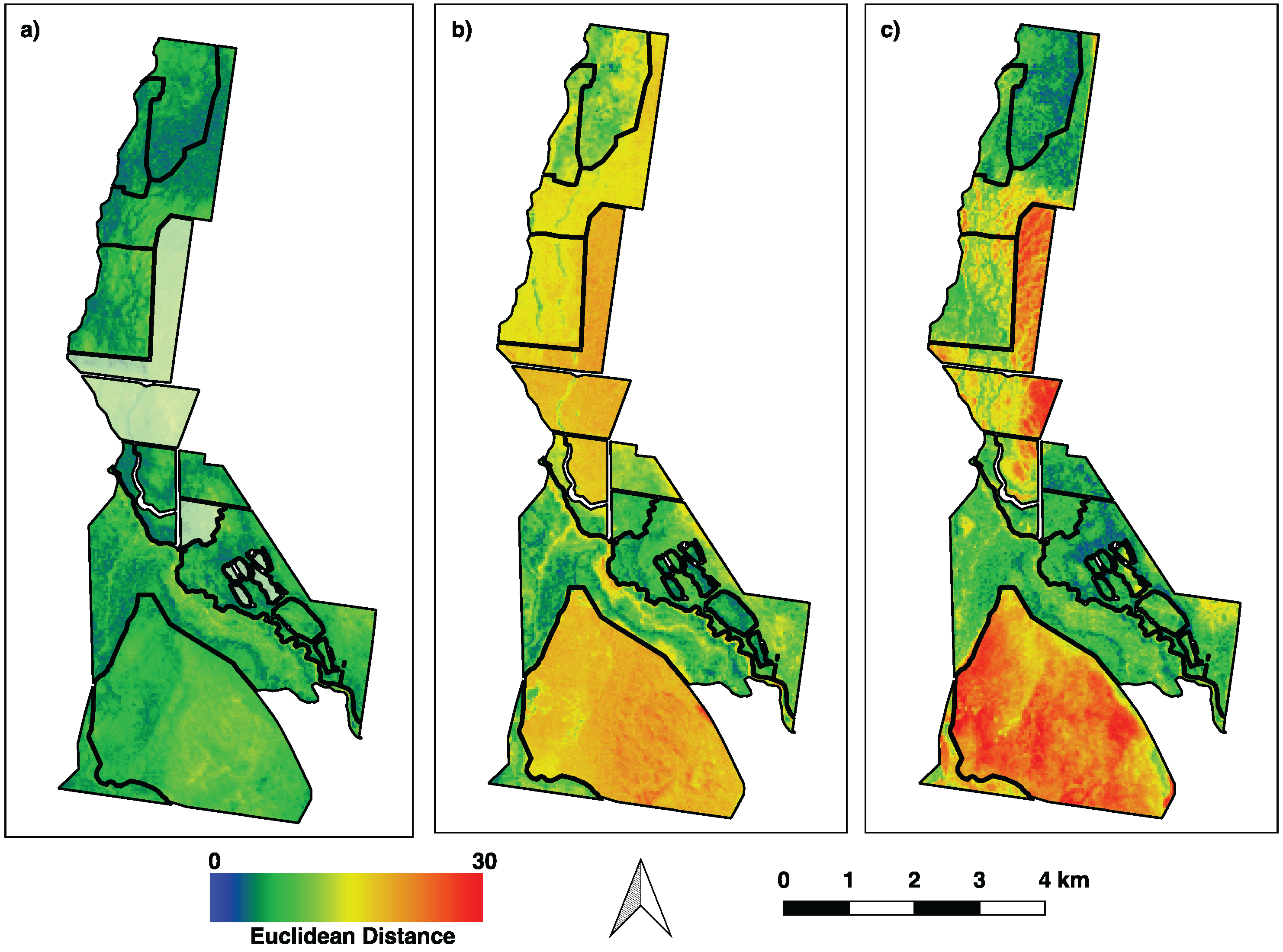
2.3. Fractional Cover Similarity Analysis
2.4. Canopy Height Model Analysis
2.5. Accuracy Testing
3. Results
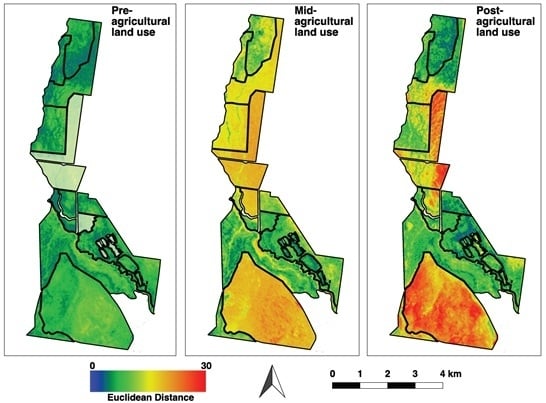
3.1. Fractional Cover
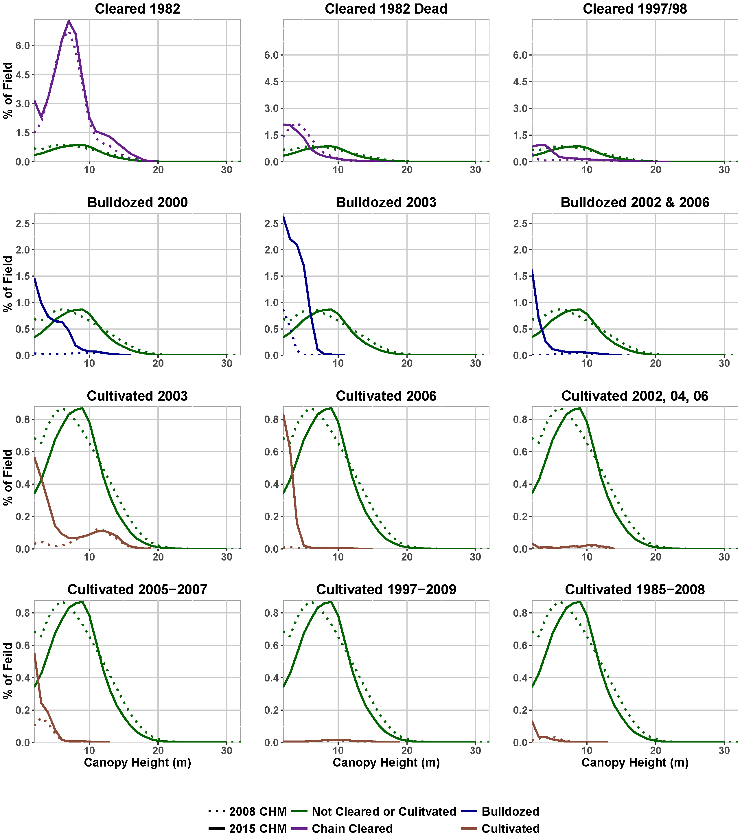
3.2. Canopy Height Models
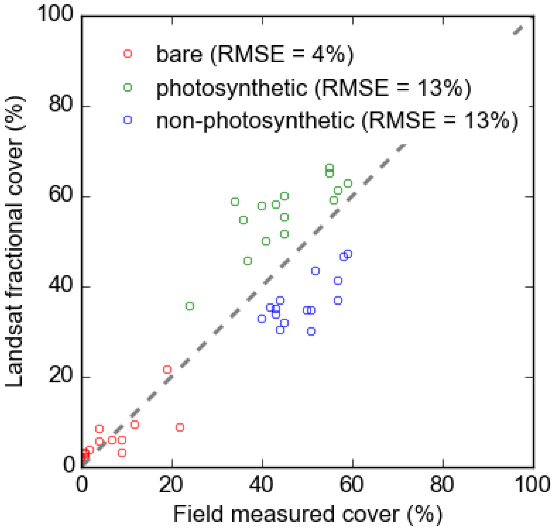
3.3. Accuracy Testing
4. Discussion
4.1. Response to Inundation and Restoration Success
4.2. Remote Sensing for Assessing Wetland Management Actions
4.3. Restoration of Pillicawarrina
5. Conclusions
Supplementary Materials
Acknowledgments
Author Contributions
Conflicts of Interest
Abbreviations
| CHM | Canopy height model |
| DEM | Digital elevation model |
References
- Tockner, K.; Stanford, J.A. Riverine flood plains: Present state and future trends. Environ. Conserv. 2002, 29, 308–330. [Google Scholar] [CrossRef]
- Millennium Ecosystem Assessment. Ecosystems and Human Well-being: Wetlands and Water; Technical Report; Island Press: Washington, DC, USA, 2005. [Google Scholar]
- Fickas, K.C.; Cohen, W.B.; Yang, Z. Landsat-based monitoring of annual wetland change in the Willamette Valley of Oregon, USA from 1972 to 2012. Wetl. Ecol. Manag. 2016, 24, 73–92. [Google Scholar] [CrossRef]
- Kingsford, R. Ecological impacts of dams, water diversions and river management on floodplain wetlands in Australia. Austral Ecol. 2000, 25, 109–127. [Google Scholar] [CrossRef]
- Moreno-Mateos, D.; Meli, P.; Vara-Rodríguez, M.I.; Aronson, J. Ecosystem response to interventions: Lessons from restored and created wetland ecosystems. J. Appl. Ecol. 2015, 52, 1528–1537. [Google Scholar] [CrossRef]
- Bernhardt, E.S.; Palmer, M.A.; Allan, J.D.; Alexander, G.; Barnas, K.; Brooks, S.; Carr, J.; Clayton, S.; Dahm, C.; Follstad-Shah, J.; et al. Synthesizing U.S. river restoration efforts. Science 2005, 308, 636–637. [Google Scholar] [CrossRef] [PubMed]
- Kearney, M.S.; Riter, J.C.A.; Turner, R.E. Freshwater river diversions for marsh restoration in Louisiana: Twenty-six years of changing vegetative cover and marsh area. Geophys. Res. Lett. 2011, 38, L16405. [Google Scholar] [CrossRef]
- Suding, K.N. Toward an Era of Restoration in Ecology: Successes, Failures, and Opportunities Ahead. Ann. Rev. Ecol. Evol. Syst. 2011, 42, 465–487. [Google Scholar] [CrossRef]
- Kennedy, R.E.; Andréfouët, S.; Cohen, W.B.; Gómez, C.; Griffiths, P.; Hais, M.; Healey, S.P.; Helmer, E.H.; Hostert, P.; Lyons, M.B.; et al. Bringing an ecological view of change to Landsat-based remote sensing. Front. Ecol. Environ. 2014, 12, 339–346. [Google Scholar] [CrossRef] [Green Version]
- Thomas, R.; Bowen, S.; Simpson, S.; Cox, S.; Sims, N.; Hunter, S.; Lu, Y. Inundation response of vegetation communities of the Macquarie Marshes in semi-arid Australia. In Ecosystem Response Modelling in the Murray Darling Basin; CSIRO Publishing: Clayton, VIC, Australia, 2010; pp. 139–150. [Google Scholar]
- Halabisky, M. Object-based classification of semi-arid wetlands. J. Appl. Remote Sens. 2011, 5, 053511. [Google Scholar] [CrossRef]
- Klemas, V. Remote Sensing of Wetlands: Case Studies Comparing Practical Techniques. J. Coast. Res. 2011, 27, 418–427. [Google Scholar] [CrossRef]
- Klemas, V. Using Remote Sensing to Select and Monitor Wetland Restoration Sites: An Overview. J. Coast. Res. 2013, 289, 958–970. [Google Scholar] [CrossRef]
- Lucas, R.M.; Blonda, P.; Bunting, P.; Jones, G.; Inglada, J.; Arias, M.; Kosmidou, V.; Petrou, Z.I.; Manakos, I.; Adamo, M.; et al. The Earth Observation Data for Habitat Monitoring (EODHAM) system. Int. J. Appl. Earth Obs. Geoinf. 2015, 37, 17–28. [Google Scholar] [CrossRef] [Green Version]
- Kayastha, N.; Thomas, V.; Galbraith, J.; Banskota, A. Monitoring Wetland Change Using Inter-Annual Landsat Time-Series Data. Wetlands 2012, 32, 1149–1162. [Google Scholar] [CrossRef]
- Guerschman, J.P.; Scarth, P.F.; McVicar, T.R.; Renzullo, L.J.; Malthus, T.J.; Stewart, J.B.; Rickards, J.E.; Trevithick, R. Assessing the effects of site heterogeneity and soil properties when unmixing photosynthetic vegetation, non-photosynthetic vegetation and bare soil fractions from Landsat and MODIS data. Remote Sens. Environ. 2015, 161, 12–26. [Google Scholar] [CrossRef]
- Hill, R.A.; Boyd, D.S.; Hopkinson, C. Relationship between canopy height and Landsat ETM+ response in lowland Amazonian rainforest. Remote Sens. Lett. 2010, 2, 203–212. [Google Scholar] [CrossRef]
- Ozesmi, S.L.; Bauer, M.E. Satellite remote sensing of wetlands. Wetl. Ecol. Manag. 2002, 10, 381–402. [Google Scholar] [CrossRef]
- Pettorelli, N.; Vik, J.O.; Mysterud, A.; Gaillard, J.M.; Tucker, C.J.; Stenseth, N.C. Using the satellite-derived NDVI to assess ecological responses to environmental change. Trends Ecol. Evol. 2005, 20, 503–510. [Google Scholar] [CrossRef] [PubMed]
- Yang, J.; Weisberg, P.J.; Bristow, N.A. Landsat remote sensing approaches for monitoring long-term tree cover dynamics in semi-arid woodlands: Comparison of vegetation indices and spectral mixture analysis. Remote Sens. Environ. 2012, 119, 62–71. [Google Scholar] [CrossRef]
- Scarth, P.F.; Röder, A.; Schmidt, M. Tracking grazing pressure and climate interaction—The role of landsat fractional cover in time series analysis. In Proceedings of the 15th Australasian Remote Sensing and Photogrammetry Conference, Alice Springs, Australia, 13–17 September 2010; p. 13.
- Huang, X.; Friedl, M.A. Distance metric-based forest cover change detection using MODIS time series. Int. J. Appl. Earth Obs. Geoinf. 2014, 29, 78–92. [Google Scholar] [CrossRef]
- Hudak, A.T.; Evans, J.S.; Stuart Smith, A.M. LiDAR Utility for Natural Resource Managers. Remote Sens. 2009, 1, 934–951. [Google Scholar] [CrossRef]
- Angelo, J.J.; Duncan, B.W.; Weishampel, J.F. Using Lidar-Derived Vegetation Profiles to Predict Time since Fire in an Oak Scrub Landscape in East-Central Florida. Remote Sens. 2010, 2, 514–525. [Google Scholar] [CrossRef]
- Akay, A.E.; Wing, M.G.; Sessions, J. Estimating structural properties of riparian forests with airborne lidar data. Int. J. Remote Sens. 2012, 33, 7010–7023. [Google Scholar] [CrossRef]
- Dufour, S.; Bernez, I.; Betbeder, J.; Corgne, S.; Hubert-Moy, L.; Nabucet, J.; Rapinel, S.; Sawtschuk, J.; Trollé, C. Monitoring restored riparian vegetation: How can recent developments in remote sensing sciences help? Knowl. Manag. Aquat. Ecosyst. 2013, 410, 10. [Google Scholar] [CrossRef]
- Chen, L.; Jin, Z.; Michishita, R.; Cai, J.; Yue, T.; Chen, B.; Xu, B. Dynamic monitoring of wetland cover changes using time-series remote sensing imagery. Ecol. Informat. 2014, 24, 17–26. [Google Scholar] [CrossRef]
- Arthington, A.H.; Pusey, B.J. Flow restoration and protection in Australian rivers. River Res. Appl. 2003, 19, 377–395. [Google Scholar] [CrossRef]
- Thomas, R.F.; Kingsford, R.T.; Lu, Y.; Cox, S.J.; Sims, N.C.; Hunter, S.J. Mapping inundation in the heterogeneous floodplain wetlands of the Macquarie Marshes, using Landsat Thematic Mapper. J. Hydrol. 2015, 524, 194–213. [Google Scholar] [CrossRef]
- Bino, G.; Sisson, S.A.; Kingsford, R.T.; Thomas, R.F.; Bowen, S. Developing state and transition models of floodplain vegetation dynamics as a tool for conservation decision-making: A case study of the Macquarie Marshes Ramsar wetland. J. Appl. Ecol. 2015, 52, 654–664. [Google Scholar] [CrossRef]
- Thomas, R.F.; Kingsford, R.T.; Lu, Y.; Hunter, S.J. Landsat mapping of annual inundation (1979–2006) of the Macquarie Marshes in semi-arid Australia. Int. J. Remote Sens. 2011, 32, 4545–4569. [Google Scholar] [CrossRef]
- Catelotti, K.; Kingsford, R.; Bino, G.; Bacon, P. Inundation requirements for persistence and recovery of river red gums (Eucalyptus camaldulensis) in semi-arid Australia. Biol. Conserv. 2015, 184, 346–356. [Google Scholar] [CrossRef]
- Department of Environment Climate Change and Water NSW. NSW Rivers Environmental Restoration Program Final Report; Technical Report; Department of Environment, Climate Change and Water NSW: Sydney, NSW, Australia, 2011. [Google Scholar]
- Kidson, R.; Witts, T.; Martin, W.; Raisin, G. Historical Vegetation Mapping of the Macquarie Marshes 1949–1991; Technical Report; NSW Department of Land and Water Conservation: Sydney, NSW, Australia, 2000. [Google Scholar]
- Waters, C. Vegetation Restoration Plan for the Pillicawarrina Floodplain; Technical Report; NSW Department of Primary Industries: Sydney, NSW, Australia, 2011. [Google Scholar]
- Paijmans, K. The Macquarie Marshes of Inland Northern New South Wales; Technical Report; Commonwealth Scientific and Industrial Research Organisation: Armidale, NSW, Australia, 1981. [Google Scholar]
- Wilson, R. Vegetation Map of the Macquarie Marshes; NSW National Parks and Wildlife Service: Sydney, NSW, Australia, 1992. [Google Scholar]
- Hall, P. Interview with Peter Hall, local grazier in the 1970s/1980s. Personal Communication, 2013. [Google Scholar]
- Flood, N.; Danaher, T.; Gill, T.; Gillingham, S. An Operational Scheme for Deriving Standardised Surface Reflectance from Landsat TM/ETM+ and SPOT HRG Imagery for Eastern Australia. Remote Sens. 2013, 5, 83–109. [Google Scholar] [CrossRef]
- Farr, T.; Rosen, P.; Caro, E.; Crippen, R.; Duren, R.; Hensley, S.; Kobrick, M.; Paller, M.; Rodriguez, E.; Roth, L.; et al. The Shuttle Radar Topography. Rev. Geophys. 2007, 45, 83–109. [Google Scholar] [CrossRef]
- Gallant, J. 1 Second SRTM Level 2 Derived Digital Surface Model (DSM) v1.0.; Technical Report; Geoscience Australia: Symonston, ACT, Australia, 2010. [Google Scholar]
- Lhermitte, S.; Verbesselt, J.; Verstraeten, W.; Coppin, P. A comparison of time series similarity measures for classification and change detection of ecosystem dynamics. Remote Sens. Environ. 2011, 115, 3129–3152. [Google Scholar] [CrossRef]
- Bowen, S.; Simpson, S. Changes in Extent and Condition of the Vegetation Communities of the Macquarie Marshes Floodplain 1991–2008; Technical Report; Final Report to NSW Wetland Recovery Program, Department of Environment, Climate Change and Water: Sydney, NSW, Australia, 2010. [Google Scholar]
- Hopkinson, C.; Chasmer, L.; Hall, R. The uncertainty in conifer plantation growth prediction from multi-temporal lidar datasets. Remote Sens. Environ. 2008, 112, 1168–1180. [Google Scholar] [CrossRef]
- Hopkinson, C.; Chasmer, L.; Lim, K.; Treitz, P.; Creed, I. Towards a universal lidar canopy height indicator. Can. J. Remote Sens. 2006, 32, 139–152. [Google Scholar] [CrossRef]
- Bunting, P.; Armston, J.; Lucas, R.; Clewley, D. Sorted pulse data (SPD) library. Part I: A generic file format for LiDAR data from pulsed laser systems in terrestrial environments. Comput. Geosci. 2013, 56, 197–206. [Google Scholar] [CrossRef]
- Bunting, P.; Armston, J.; Clewley, D.; Lucas, R. Sorted pulse data (SPD) library—Part II: A processing framework for LiDAR data from pulsed laser systems in terrestrial environments. Comput. Geosci. 2013, 56, 207–215. [Google Scholar] [CrossRef]
- Andersen, H.E.; Reutebuch, S.; McGaughey, R.; d’Oliveira, M.; Keller, M. Monitoring selective logging in western Amazonia with repeat lidar flights. Remote Sens. Environ. 2014, 151, 157–165. [Google Scholar] [CrossRef]
- Vepakomma, U.; St-Onge, B.; Kneeshaw, D. Spatially explicit characterization of boreal forest gap dynamics using multi-temporal lidar data. Remote Sens. Environ. 2008, 143, 2326–2340. [Google Scholar] [CrossRef]
- Hijmans, R.; van Etten, J. Raster: Geographic Analysis and Modeling with Raster Data. R Package Version 2.0-12. 2012. Available online: https://cran.r-project.org/src/contrib/Archive/raster/ (accessed on 16 June 2016).
- R Development Core Team. R: A Language and Environment for Statistical Computing; R Foundation for Statistical Computing: Vienna, Austria, 2015. [Google Scholar]
- Royal Botanic Gardens And Domain Trust. PlantNET–New South Wales, Flora Online, 2015. Available online: http://plantnet.rbgsyd.nsw.gov.au/ (accessed on 16 June 2016).
- Muir, J.; Schmidt, M.; Tindall, D.; Trvithick, R.; Scarth, P.; Stewart, J. Field Measurement of Fractional Ground Cover: A Technical Handbook Supporting Ground Cover Monitoring for Australia; Technical Report; Prepared by the Queensland Department of Environment and Resource Management for the Australian Bureau of Agricultural and Resource Economics and Sciences: Canberra, ACT, Australia, 2011. [Google Scholar]
- Roberts, J.; Marston, F. Water Regime for Wetland and Floodplain Plants; National Water Commission: Canberra, ACT, Australia, 2011; p. 180. [Google Scholar]
- Melesse, A.M.; Nangia, V.; Wang, X.; McClain, M. Wetland Restoration Response Analysis Using MODIS and Groundwater Data. Sensors 2007, 7, 1916–1933. [Google Scholar] [CrossRef]
- George, A.K.; Walker, K.F.; Lewis, M.M. Population status of eucalypt trees on the River Murray floodplain, South Australia. River Res. Appl. 2005, 21, 271–282. [Google Scholar] [CrossRef]


| Field Name | Land Use History |
|---|---|
| Never cleared | Never cleared or cultivated |
| Cleared (1982-healthy) | Chain cleared 1982 |
| Cleared (1982-dead) | Chain cleared 1982, but now comprised of dead river cooba overstorey and grass understory |
| Cleared (1997/1998) | Comprised of three similar fields cleared in: (1) 1982 and 98, (2) 1986 and 98, (3) 1997 |
| Bulldozed (2000) | Bulldozed 2000 |
| Bulldozed (2003) | Bulldozed and ploughed 2003 |
| Bulldozed (2002 and 2006) | Bulldozed 2002, ploughed 2006 |
| Cultivated (2003) | Levelled 2002, cultivated 2003 |
| Cultivated (2006) | Levelled 2006, cultivated 2006 |
| Cultivated (2002, 2004, 2006) | Levelled 2002, cultivated 2002, 2004 and 2006 |
| Cultivated (2005–2007) | Bulldozed 2002, levelled 2003, cultivated 2005–2007 |
| Cultivated (1997–2009) | Levelled 1997, cultivated 1997–2009 |
| Cultivated (1985–2008) | Cleared 1985, cultivated 1985–2009 |
| Field Name | Pre-Devel. | Peak-Devel. | After-Rest. | |||||
|---|---|---|---|---|---|---|---|---|
| Mean | SD | Mean | SD | Δ | Mean | SD | Δ | |
| Never cleared | 7.31 | ±1.89 | 9.45 | ±3.38 | 2.14 | 10.15 | ±3.73 | 2.84 |
| Cleared 1982 healthy | NA | 8.35 | ±1.44 | NA | 7.9 | ±1.23 | NA | |
| Cleared 1982 dead | NA | 6.22 | ±1.7 | NA | 8.83 | ±3.1 | NA | |
| Cleared 1997/1998 | 7.05 | ±1.69 | 9.73 | ±2.44 | 2.68 | 7.84 | ±2.93 | 0.79 |
| Bulldozed 2000 | 5.78 | ±1.15 | 12.16 | ±2.47 | 6.38 | 6.06 | ±1.72 | 0.28 |
| Bulldozed 2003 | 6.91 | ±1.64 | 12.63 | ±1.75 | 5.45 | 6.65 | ±2.16 | −0.26 |
| Bulldozed 2002 and 2006 | 5.37 | ±0.92 | 12.69 | ±1.98 | 7.32 | 8.17 | ±2.24 | 3.34 |
| Cultivated 2003 | 5.32 | ±1.11 | 11.82 | ±2.77 | 6.5 | 9.62 | ±2.33 | 4.3 |
| Cultivated 2006 | 6.14 | ±1.16 | 16.29 | ±1.23 | 10.15 | 11.54 | ±4.91 | 5.4 |
| Cultivated 2002, 2004, 2006 | 6.5 | ±1.52 | 17.98 | ±0.88 | 11.48 | 15.87 | ±4.09 | 9.37 |
| Cultivated 2005–2007 | 7.12 | ±1.8 | 16.17 | ±1.4 | 9.05 | 12.31 | ±3.23 | 5.19 |
| Cultivated 1997–2009 | 8.66 | ±1.62 | 19.34 | ±1.69 | 10.86 | 22.58 | ±3.43 | 13.92 |
| Cultivated 1985–2008 | NA | 19.14 | ±1.33 | NA | 19.67 | ±4.94 | NA | |
| Field Name | Land Use History |
|---|---|
| Never cleared | Largely comprised or river red gum forest, with smaller patches of lignum and occasional river cooba stands and grasslands |
| Cleared (1982-healthy) | Densely forested with river red gum, river cooba and lignum all co-occurring |
| Cleared (1982-dead) | Densely forested with river cooba, which is largely dead, grassland understorey |
| Cleared (1997/1998) | River cooba makes up the overstorey majority, with occasional lignum plants and grassland understorey |
| Bulldozed (2000) | River cooba stands, patches of lignum, some reeds and rushes, some grasslands with (mostly) wetland species, occasional mature river red gum trees |
| Bulldozed (2003) | Lignum patches and smaller stands of river cooba with grasslands in areas observed to be drier |
| Bulldozed (2002 and 2006) | Some dense river cooba stands, patches of lignum and river red gum, occasional older trees |
| Cultivated (2003) | River cooba and river red gum saplings, occasional patches of reeds (observed wetter areas) and grasslands (observed drier areas) |
| Cultivated (2006) | Some dense river cooba stands, patches of reeds, rushes and grasslands (mainly wetland species), some lignum |
| Cultivated (2002, 2004, 2006) | Largely grasslands (mostly drier/terrestrial species with some patches of wetland species), occasional river cooba or river red gum trees |
| Cultivated (2005–2007) | Bulldozed 2002, levelled 2003, cultivated 2005–2007 |
| Cultivated (1997–2009) | Largely grasslands (mostly drier/terrestrial species with some patches of wetland species), a very few river red gum trees from pre-cultivation still present |
| Cultivated (1985–2008) | Largely grasslands (terrestrial and wetland patches) occasional river cooba or lignum plants, small dense stands of river red gum saplings in channel lines |
© 2016 by the authors; licensee MDPI, Basel, Switzerland. This article is an open access article distributed under the terms and conditions of the Creative Commons Attribution (CC-BY) license (http://creativecommons.org/licenses/by/4.0/).
Share and Cite
Dawson, S.K.; Fisher, A.; Lucas, R.; Hutchinson, D.K.; Berney, P.; Keith, D.; Catford, J.A.; Kingsford, R.T. Remote Sensing Measures Restoration Successes, but Canopy Heights Lag in Restoring Floodplain Vegetation. Remote Sens. 2016, 8, 542. https://doi.org/10.3390/rs8070542
Dawson SK, Fisher A, Lucas R, Hutchinson DK, Berney P, Keith D, Catford JA, Kingsford RT. Remote Sensing Measures Restoration Successes, but Canopy Heights Lag in Restoring Floodplain Vegetation. Remote Sensing. 2016; 8(7):542. https://doi.org/10.3390/rs8070542
Chicago/Turabian StyleDawson, Samantha K., Adrian Fisher, Richard Lucas, David K. Hutchinson, Peter Berney, David Keith, Jane A. Catford, and Richard T. Kingsford. 2016. "Remote Sensing Measures Restoration Successes, but Canopy Heights Lag in Restoring Floodplain Vegetation" Remote Sensing 8, no. 7: 542. https://doi.org/10.3390/rs8070542