

Abstract
International climate mitigation efforts are focused on limiting increase in global mean temperature, which has been shown to be proportional to cumulative CO2 emissions. However, the ability of natural and human systems to successfully adapt to climatic changes depends on both the magnitude and rate of change, the latter of which will depend on how quickly a given level of cumulative emissions occurs. We show that cumulative CO2 emissions of 4620 Gt CO2 (reached in 2100 in RCP4.5 and 2057 in RCP8.5) produce globally averaged warming rates that are nearly twice as fast in RCP8.5 than RCP4.5 (0.34 ± 0.08 °C per decade versus 0.19 ± 0.05 °C per decade, respectively). Similarly, the globally averaged velocity of climate change calculated according to the 'nearest equivalent climate' is greater by a factor of ∼2 in RCP8.5 than in RCP4.5 (2.51 ± 0.67 km yr−1 versus 1.32 ± 0.39 km yr−1, respectively), despite equivalent cumulative emissions. These differences in the projected velocity of climate change represent uncertainty for ecosystems that may be unable to adapt to the faster changes. Particularly at risk are boreal forests, of which 48% are projected to experience rates of change beyond their expected adaptive capacity (i.e. >0.3 °C per decade) in RCP4.5, compared with 95% in RCP8.5. Thus, the same budget of cumulative carbon emissions may result in critically different impacts on natural and human systems, depending on the amount of time over which that budget is expended.
Export citation and abstract BibTeX RIS

Content from this work may be used under the terms of the Creative Commons Attribution 3.0 licence. Any further distribution of this work must maintain attribution to the author(s) and the title of the work, journal citation and DOI.
1. Introduction
Projected rates of global warming in the 21st century exceed any known global-scale warming event in the past 50 million years [1, 2]. Such rapid warming poses serious threats to global ecosystems and biodiversity given biophysical limits in the ability of systems and species to adapt to the impacts of climate change. In this context, adaptation is defined broadly to include migration as well as genetic or behavioral changes in response to climate change. Limits to adaptation vary widely across ecosystems and species, but many studies have found the rate of warming to be a key determinant of climate impacts on natural systems [3–8]. This is because successful adaptation of endemic species through behavioral and/or genetic changes [9, 10] must occur at the same rate or faster than ecosystem areas are changing. For instance, Leemans and Eickhout [4] find that warming of 0.1 °C per decade may be within the capacity of roughly 50% of ecosystems to keep pace with warming, but that only 30% of ecosystems could successfully keep pace with warming of 0.3 °C per decade [4]. Species may respond to climate change by shifting their ranges (e.g., poleward or to higher elevations) [11–13]. For example, fossil pollen indicates that tree species shifted poleward at speeds of up to 10 km per decade to keep pace with postglacial global warming [14, 15]. Such dynamic responses to climate change are critical for species to maintain equilibrium with climate [16]. Researchers have therefore begun to compare observed migration rates with the projected velocity of future climate change, or the distance per unit time that organisms would need to migrate in order to maintain an equivalent climate [2, 11, 17]. Ecosystems and species that are unable to adapt or migrate to keep pace with climate changes face reduced fitness and local collapse or extinction. Further, although less studied, the physical, sociopolitical and economic capacities of some human systems (e.g., agriculture, water management) to respond to climate change are also potentially sensitive to the rates and pace of climate change [18–23].
While climate impacts are likely to be strongly influenced by the rate of climate change, a series of prominent studies have emphasized that peak warming of global mean temperatures is not dependent on anthropogenic emissions pathway, but will be proportional to cumulative CO2 emissions since the pre-industrial era [24–27]. For example, if cumulative emissions after 1860 are kept below 3500 Gt CO2 (955 Gt C), there is a 50% probability of staying below a 2 °C temperature threshold [28].
Given the simplicity and robustness of the transient climate response to cumulative CO2 emissions, an increasing number of analysts have proposed using quotas of cumulative emissions as a basis for climate policy, for instance by agreeing upon a cumulative carbon budget to be shared across space and time [28–31]. However, others have criticized the narrow focus on global mean temperature as an incomplete indicator of the 'dangerous anthropogenic interference in the climate system' that the United Nations Framework Convention on Climate Change aims to avoid [e.g., 32]. Indeed, a goal of the UNFCCC is that a stable level of atmospheric CO2 'should be achieved within a time-frame sufficient to allow ecosystems to adapt naturally to climate change' [33]. However, despite this emphasis in the UN framework, relatively little attention has been paid to the dependence of climate velocities on emissions pathways [34, 35].
Here, we assess differences in future warming rates and climate velocities when cumulative emissions are equivalent but emissions pathways have diverged. We then compare these rates across the Earth's major biomes, and discuss the implications of the projected differences in rate of change within a fixed cumulative emissions budget.
2. Materials and methods
2.1. Emissions pathways
The Representative Concentration Pathways developed for the climate modeling community span a large range of radiative forcing in the year 2100, and thus a similarly large range of cumulative emissions [36]. In order to compare warming rates and velocities for the same level of cumulative emissions, we compare a pathway with projections exceeding 4 °C of warming in 2100 (RCP8.5), with a more moderate pathway with projections avoiding 3 °C of warming in 2100 (RCP4.5). As shown in figure 1, RCP8.5 reaches the same level of cumulative CO2 emissions in 2057 that RCP4.5 reaches in 2100 (4620 Gt CO2 since 1850). Thus, the two RCPs represent unique trajectories of annual emissions whose cumulative total is equivalent at different points in time.

Figure 1. Cumulative emissions in RCP4.5 and RCP8.5 from 1850. A total of 4620 Gt CO2 are emitted between 1850 and 2100 in RCP4.5. The same cumulative total is reached in 2057 in RCP8.5.
Download figure:
Standard image High-resolution imageAlthough the RCPs include forcing from short-lived, non-CO2 greenhouse gases, recent studies have shown that—contrary to earlier studies [e.g., 37, 38]—the warming avoided by reducing emissions of these short-lived climate forcers is likely to be small [39, 40]. Therefore, we focus on cumulative CO2 emissions.
2.2. Model simulations
We calculate climate velocities following Diffenbaugh and Field [2], who identified the closest grid cell with a future mean annual temperature that is statistically identical to that of the baseline mean annual temperature [2]. Using this method with low-resolution global climate model simulations may overestimate velocities in mountainous areas [17]. However, it is less dependent on current gradients of surface temperature than other methods, and thereby incorporates the fact that temperature is likely to change over broad spatial scales, which will increase the distance needed to maintain the present climate envelope [2], even in mountainous regions (figure S4). We make three important updates to the method of Diffenbaugh and Field. First, we define the equivalent climate using Student's t-test. As a result, for each grid cell Gpresent, the distance term in the climate velocity is calculated as the distance to the nearest grid cell Gfuture for which the current population of annual temperatures at Gpresent and the future population of annual temperatures at Gfuture are not statistically distinguishable at the 95% confidence level. Second, we use the climate at the time horizon at which the target cumulative emissions level is reached, meaning that the time term in the climate velocity is the number of years needed to reach the target cumulative emissions level in a given RCP. Third, we calculate the climate velocity for each climate model individually, and then analyze the distribution of projected velocity values at each grid point.
We analyze climate model simulations from the CMIP5 archive [41]. Our approach to aggregating the CMIP5 climate models balances four constraints: (1) maximizing the population size for calculating the statistical significance of changes in temperature, (2) maximizing the number of CMIP5 models analyzed, (3) minimizing the slope of cumulative emissions within the target time horizon, and (4) conducting the analysis at a spatial scale that is similar to the original grid size of CMIP5 climate models. To balance these three constraints, we analyze simulated temperature from those CMIP5 climate models that have archived at least 4 realizations in the historical, RCP4.5 and RCP8.5 experiments (table S1). Following numerous previous studies (e.g. Giogi 2006), we first interpolate the temperature data from each CMIP5 model to a common 1 × 1 geographical grid. We then create a 20-year population for each model in each time horizon by pooling the annual temperatures from a 5-year period in 4 realizations of each model (4 realizations × 5 years per realization = 20 years). These individual-model populations include a 20-year baseline pool from the last 5 years of the CMIP5 historical simulation (2001–2005), a 20-year future pool from the 5 years ending in the year that the target cumulative emissions of 4620 Gt CO2 are reached in RCP4.5 (2096–2100), and a 20-year future pool from the 5 years ending in the year that the target cumulative emissions of 4620 Gt CO2 are reached in RCP8.5 (2053–2057).
Because we analyze RCP emission pathways, some warming may be the result of non-CO2 greenhouse gases, and thus not accounted for in cumulative CO2 emissions alone (see [42]). However, we find that the temperature differences between RCP4.5 and RCP8.5 emission pathways are small for a given level of cumulative emissions, particularly when compared with the differences between individual models (figure S1). Additionally, we see spatial variability in warming trends, indicating that warming will not be uniform over all areas of the Earth. Thus, climate risks will depend on both warming, and the unique assemblage of biotic and abiotic factors characteristic of large units of land over which warming occurs. These large units land with distinct characteristics have been defined as Earth's major terrestrial biomes. Following Loarie et al and Mahlstein et al [17, 43], we evaluate warming rates and velocities for each biome using a detailed map of 14 major biomes as they exist now [43, 44] (figure S2). We compute warming rates as decadal temperature difference between the five-year baseline (2001–2005) period and the five-year period at which the cumulative emissions target is reached.
Although the 1 × 1 grid on which we calculate climate velocities is a finer spatial resolution than most of the CMIP5 climate models, it is a much more coarse resolution than the actual spatial heterogeneity of temperature. In order to test whether our use of a 1 × 1 grid overestimates the local extirpation of current annual temperature, we use the high-resolution WorldClim data [45] to calculate the fraction of 10 min grid cells from the WorldClim historical temperature data which no longer exist within the corresponding 1-degree grid box in the WorldClim RCP8.5 2050 climate (figure S4).
3. Results
3.1. Global rate of warming and velocity of climate change
Averaged globally, the decadal warming rate in RCP8.5 is 0.34 ± 0.08 °C per decade, which is nearly double the mean rate of 0.19 ± 0.05 °C per decade projected in RCP4.5 (figures 2(C) and (D)). Assessing the trends in warming rates over each decade in the two pathways, we find that mean warming rates in both RCP4.5 and RCP8.5 are comparable and greater than 0.2 °C per decade until 2040, after which the rates diverge sharply, slowly decreasing to about 0.1 °C per decade by 2071–2080 in RCP4.5, but increasing to as much as 0.5 °C per decade in RCP8.5 (figure S3).

Figure 2. Maps showing the difference in the median warming relative to baseline in RCP 4.5 (A) and RCP8.5 (B), median warming rate in RCP4.5 (C) and RCP8.5 (D), and climate velocity (E and F) in RCP4.5 and 8.5 when cumulative CO2 emissions are 4620 Gt CO2. (2006–2100 in RCP4.5 and 2006–2057 in RCP8.5; see figure 1).
Download figure:
Standard image High-resolution imagePanels E and F of figure 2 show median climate velocities projected in RCP4.5 and RCP8.5, respectively, under equivalent cumulative CO2 emissions of 4620 Gt CO2. As in the case of warming rates, the differences in globally averaged velocities are substantial: the mean velocity is a factor of ∼2 greater in RCP8.5 (2.5 ± 0.7 km per year) than in RCP4.5 (1.3 ± 0.4 km per year). As in Diffenbaugh and Field [2], the highest velocities are seen at the poleward edges of continents and in regions of high elevation, where the equivalent climate must be found far afield once the temperature moves 'off the edge' of the continent or 'off the top' of mountains. These large velocities therefore represent the effects of substantial latitudinal and/or longitudinal displacements of the equivalent annual temperature.
The velocities that we calculate are in some cases considerably larger than those calculated using methods that utilize the local temperature gradients [e.g., 17], but are more similar in magnitude to those calculated using methods based on bioclimatic projections of suitable climate envelopes [e.g., 46]. Given the persistent contrast in the literature between velocities calculated using the present local gradients and velocities calculated using the nearest suitable location in the future climate, it is worth noting a few features of our implementation of the nearest-suitable-location approach, both when considering our raw velocity values and when considering the ecosystem velocity values reported below:
- First, because our approach accounts for changes in climate outside of the local vicinity, it accounts for changes in regional temperature that can be missed in methods that only focus on the local temperature gradients that exist in the present climate [2].
- Second, as noted in Diffenbaugh and Field, some of the large velocities identified in high elevation areas could be ameliorated by the presence of areas of temperature 'refugia' that can be created by complex topography (as identified in Loarie et al [17]). As a result, particularly in mountainous regions, there are likely to be some areas of refugia that will afford the opportunity for smaller velocities than those reported here. In particular, while previous 'local gradient' calculations are likely biased low by ignoring all temperature changes outside of the hyper-local area on a very high-resolution grid, our calculated velocities could be biased high by the fact that we conduct our analysis on a 1 × 1 grid: Although our method requires that temperature changes be statistically significant at the 95% confidence level (meaning that the future temperature at a grid cell must fall substantially outside of that grid cell's historical variability in order for a given grid cell to be required to relocate), the fact that the grid cells are separated by approximately 100 km potentially sets an artificial minimum on the calculated velocities of relocated grid cells by not accounting for the spatial heterogeneity of temperature within each 1 × 1 grid cell.
As a preliminary test of the sensitivity of calculated velocities to grid resolution, we analyze the historical and projected annual temperatures provided by WorldClim at 10 min spatial resolution (about 18.5 km at the equator) [17, 45]. We compare the observed historical WorldClim annual temperature dataset with the CMIP5 GCMs available from WorldClim (table S2) for the 2041–2060 period of RCP8.5 (which is a similar cumulative emissions window as our RCP8.5 window of 2053–2057). Using the WorldClim data, we quantify the percentage of 10 min grid cells in which the present annual temperature no longer exists within the corresponding 1-degree grid box in the future climate, and is therefore 'extirpated' from the corresponding 1-degree grid box (figure S4). Over most of the world, the greater spatial resolution has surprisingly little effect, with the historical annual temperature no longer existing within the corresponding 1-degree grid box in the future climate for >90% of the 10 min grid cells over much of the globe. As expected, greater potential for refugia exists in mountainous areas, which in many cases exhibit a smaller fraction of 10 min grid cells whose historical annual temperature is extirpated from the starting 1-degree grid box in the future climate. However, most mountainous areas still exhibit at least 30% extirpation of 10 min historical temperature, and some exhibit >90% (figure S4). These temperature extirpation percentages suggest that the high velocities calculated by our equivalent-temperature method are not entirely an artifact of the 1-degree resolution at which we perform the calculation. In addition, it should be noted that our sensitivity analysis is conservative in that it does not constrain the area available in each temperature window. In reality, while temperature refugia preserved by mountainous terrain are likely to provide some relief from very high velocity migration, they are unlikely to be sufficiently large to preserve equivalent geographic area. Future comparisons of methods for calculating climate change velocity should therefore consider both the sensitivity to spatial resolution and the velocity required to maintain the equivalent area currently occupied by different biomes.
- Third, our velocity calculation only accounts for large-scale changes in the regional and global temperature patterns, and does not account for changes in other climate variables or for fragmentation of the landscape. In practice, organisms 'tracking' these temperature changes would encounter a range of multivariate climate surfaces overlain on a highly fragmented landscape, which would likely create substantial barriers to successful migration [46].
Given all of these caveats, our velocity calculations should be considered a comparison of the rate of large-scale temperature change within fast and slow pathways to a given level of cumulative emissions, and not as predictions of the likelihood of complete extirpation of a climate envelope from a given region nor as predictions of achievable migration within the current human-dominated landscape.
3.2. Rate of warming and velocity of climate change in specific biomes
Figure 3 summarizes the ranges of warming rates experienced by different biomes for the same level of cumulative emissions projected in RCP4.5 and RCP8.5, ranked by the difference in median rates of temperature increase per decade between the emission pathways. The histograms reveal particularly large differences in pathway warming rates (∼0.25 °C per decade) in high latitude biomes such as boreal forests and tundra, which is where warming rates are also the fastest. Differences in median warming rates between RCP4.5 and RCP8.5 are >0.1 °C per decade in all of the assessed biomes (p < 0.01; figure 3, tables S3 and S4). Also evident in figure 3 is the considerably larger variability of warming rates projected in RCP8.5 (1σ = 0.08 °C per decade globally) than in RCP4.5 (1σ = 0.05 °C per decade globally), reflecting an increase in the higher rates of warming in RCP8.5.
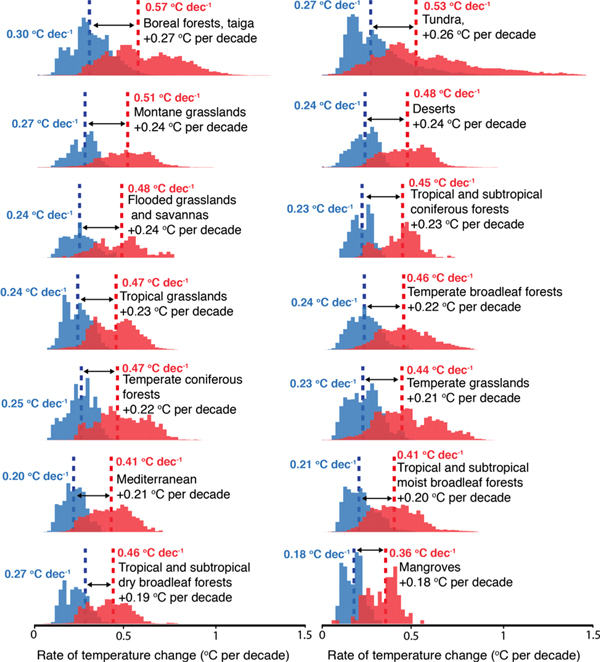
Figure 3. Histograms of decadal warming rates by biome in RCP4.5 (blue) and RCP8.5 (red) when cumulative carbon emissions are equal (4620 Gt CO2; see figure 1). Dashed lines indicate median warming rates in °C per decade, and these median values are indicated in blue and red text for RCP4.5 and RCP8.5, respectively. The difference in these median warming rates are also indicated in the biome labels. Histograms are ordered by difference in warming rate between RCP4.5 and RCP8.5 pathways.
Download figure:
Standard image High-resolution imageAnalogously, figure 4 shows differences in the distribution of climate velocities by biome between RCP4.5 and RCP8.5 in the year that each reach the same level of cumulative emissions, ranked by the difference in median velocities. Again, we find the largest pathway differences in velocity occur in high latitude tundra and boreal forests, where median velocities increase by >5 km yr−1 in RCP8.5 compared to >3 km yr−1 in RCP4.5 (figure 4). However, in the case of velocities, we also find large differences in both temperate coniferous (3.4 km yr−1) and tropical moist broadleaf (3.2 km yr−1) forests. We reiterate that the equivalent climate method we use in general results in velocities that are much greater than previous studies (see discussion in section 3.1). For example, we find a median velocity in the tundra biome for RCP4.5 of 3.6 km yr−1, more than an order of magnitude greater than the velocity for the same biome reported by Loarie et al (0.29 km yr−1) using a method based on present-day surface temperature gradients [17].
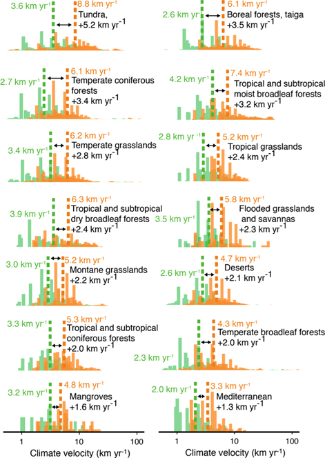
Figure 4. Histograms of climate velocities by biome in RCP4.5 (green) and RCP8.5 (orange) when cumulative carbon emissions are equal (4620 Gt CO2; see figure 1). Dashed lines indicate median velocities in km per year, and these median values are indicated in green and orange for RCP4.5 and RCP8.5, respectively. The difference in median velocities is also indicated in the biome labels. Histograms are ordered by difference in warming rate between RCP4.5 and RCP8.5 pathways.
Download figure:
Standard image High-resolution image3.3. Areas of biomes where projected rates and pace of warming are extreme
Previous studies of the transient ecological response to climate change have estimated the adaptive capacity of ecosystems at threshold warming rates [4, 47]. For example, an analysis by Leemans and Eikhout suggested that forest ecosystems are the biome that is most sensitive to rates of temperature change, estimating that 36% and 17% of impacted forests could keep pace with 0.1 °C and 0.3 °C warming per decade, respectively [4]. Neilson, meanwhile, found evidence that all ecosystems decline at warming rates greater than 0.4 °C per decade [47].
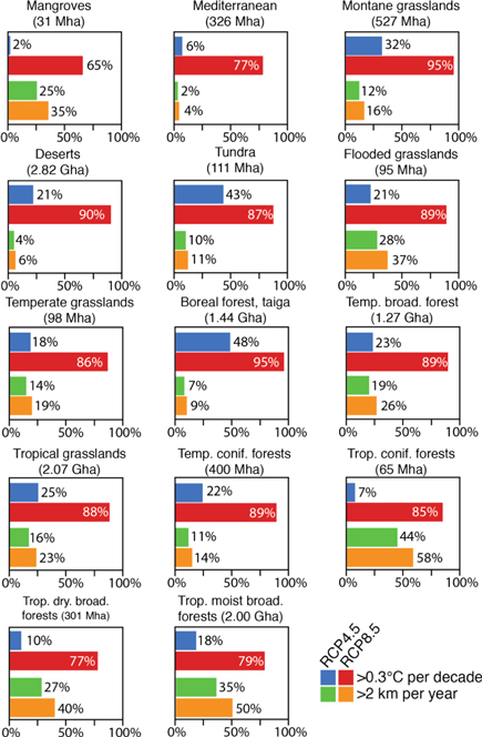
Figure 5 shows the areal percentages of each biome that avoid warming thresholds of 0.3 °C per decade and velocities of 2 km yr−1, which loosely correspond to thresholds for high climate impacts identified in previous studies. In all biomes, despite the same cumulative CO2 emissions, the areas where warming rates exceed 0.3 °C warming per decade in RCP4.5 are smaller than the areas where warming rates exceed 0.3 °C per decade in RCP8.5 (figure 5). This suggests that emitting more CO2 in the near-term will increase both the area and intensity of climate impacts in most biomes. This is especially true for high latitude biomes, such as tundra and boreal forest, where the proportion of these biomes projected to exceed 0.3 °C per decade is 31%–48% in RCP4.5, compared to 94%–95% in RCP8.5 (figure 5). Similarly, the areas of each biome with climate velocities exceeding 2 km yr−1 are consistently larger in the RCP8.5 emissions pathway than in the RCP4.5 emissions pathway. For example, 27% of tropical dry broadleaf forests experience climate velocities greater than 2 km yr−1 in RCP4.5, while 40% are greater than 2 km yr−1 in RCP8.5 (figure 5). (We note that our use of a 1 × 1 grid for the equivalent temperature calculation does not appear to artificially exceed the 2 km yr−1 threshold, as most areas of the globe exhibit at least some extirpation of the historical 10 min temperature outside of the original 1 × 1 (∼100 km) grid box within a half-century in RCP8.5; figure S4.)
Figure 5. Areal percentages of each biome where projected warming rates exceed 0.3 °C per decade in RCP4.5 (blue) and RCP8.5 (red), and where projected climate velocities exceed 2 km per year in RCP4.5 (green) and RCP8.5 (orange) when cumulative carbon emissions are equal (4620 Gt CO2; see figure 1).
Download figure:
Standard image High-resolution image
4. Discussion and conclusions
Our results demonstrate that the rate of warming and velocity of climate change caused by a cumulative total of carbon emissions can vary drastically depending on the pathway of emissions. This variation is important because in many cases the capacity of human and natural systems to adapt or migrate may be limited by these rates as much as by the overall level of change [46, 48–52]. Indeed, the magnitude and areal extent of differences in warming rates and climate velocities projected under the same cumulative emissions in RCP4.5 and RCP8.5 are sufficiently large that many ecosystems and species which may be able to adapt or shift in response to the slower, isolated changes could be challenged to persist in the face of the faster, more widespread changes (see figure 5).
Differences in rates of change under the same level of cumulative emissions are particularly large in high latitude biomes of tundra and boreal forest, but are substantial and statistically significant everywhere (tables S3 and S4). The differences of warming rates and velocities for equivalent cumulative emissions are mostly a result of equivalent warming occurring over a much shorter amount of time, suggesting that emitting large amounts of carbon in the near-term will cause extremely fast changes in some areas. The long tails in the histograms in figures 3 and 4 indicate areas that may experience such rapid change. For example, the maximum warming rates and velocities projected in tundra are ∼1 °C per decade and ∼40 km yr−1 in RCP4.5, respectively, but jump to nearly 1.5 °C per decade and ∼70 km yr−1 in RCP8.5 (see figures 3 and 4). The variation and spread of warming rates and climate velocities within biomes is a result of both inter-model variability (see figure S1), and spatial differences in warming patterns (see figure 2). If extremes are realized, such rates of change are much greater than the adaptive capacities of organisms discussed in the literature, and, in some cases, could lead to local extinctions and ecosystem collapse [22]. The responses of ecosystems and species to warming rate and climate velocity could be even more severe in areas fragmented by human and natural barriers [11, 53].
To the extent that some climate impacts are dependent on the pathway of carbon emissions, cumulative emissions and the mean level of warming are an incomplete basis for climate policy. Rather, because rates of warming are closely correlated with peak annual emissions [35], our results suggest that limiting future growth of annual emissions may greatly improve the chances that human and natural systems will successfully respond to climate change through either local adaptation or migration. While the response of terrestrial ecosystems to climate change will be dependent on many factors, including precipitation, atmospheric CO2, and nutrient availability, our analysis reveals that lower emissions trajectories would decrease the overall costs of climate mitigation [e.g., 54] and reduce the risks of relying on negative emissions [55] or intentional climate interventions [56] later in the century. We note that our analysis does not take into account the effects of short-lived climate pollutants (SLCPs), mitigation of which may have the potential to slow warming rates in the near term. Indeed, it can be argued that the best mitigation strategy would address both long-term and near-term warming through limiting both SLCPs and CO2 emissions [57]. However, if policy efforts to mitigate SLCPs distract from efforts to limit CO2 emissions, rates of warming will inevitably increase in the long term. Additionally, others have argued that the same policy efforts that reduce CO2 emissions will simultaneously reduce SLCP emissions without additional policy [39].
The amount of global warming that will occur in the future is an important indicator of future climate impacts, and the proportionality of that warming to cumulative carbon emissions is thus a convenient basis to connect those future climate impacts to national and technological sources of carbon emissions. However, a singular focus on the overall level warming and the corresponding budget of cumulative emissions neglects other critical indicators of 'dangerous anthropogenic interference,' such as the rate of warming and velocity of climate change, both of which are sensitive to the emissions pathway. Mitigation efforts that explicitly limit annual emissions may therefore be more effective in avoiding climate impacts than those that only set a cumulative emissions quota, because the rate at which CO2 is added to the atmosphere may ultimately determine whether human and natural systems can keep pace with climate change.
Acknowledgments
We thank Ken Caldeira, Stéphane Hallegatte, and Michael Mastrandrea for their insightful comments and suggestions. We also thank the editors of this special issue for inviting our contribution to this special issue.