

Abstract
Methane (CH4) is a potent greenhouse gas (GHG) that affects the global climate system. Knowledge about land–atmospheric CH4 exchanges on the Qinghai-Tibetan Plateau (QTP) is insufficient. Using a coupled biogeochemistry model, this study analyzes the net exchanges of CH4 and CO2 over the QTP for the period of 1979–2100. Our simulations show that the region currently acts as a net CH4 source with 0.95 Tg CH4 y−1 emissions and 0.19 Tg CH4 y−1 soil uptake, and a photosynthesis C sink of 14.1 Tg C y−1. By accounting for the net CH4 emission and the net CO2 sequestration since 1979, the region was found to be initially a warming source until the 2010s with a positive instantaneous radiative forcing peak in the 1990s. In response to future climate change projected by multiple global climate models (GCMs) under four representative concentration pathway (RCP) scenarios, the regional source of CH4 to the atmosphere will increase by 15–77% at the end of this century. Net ecosystem production (NEP) will continually increase from the near neutral state to around 40 Tg C y−1 under all RCPs except RCP8.5. Spatially, CH4 emission or uptake will be noticeably enhanced under all RCPs over most of the QTP, while statistically significant NEP changes over a large-scale will only appear under RCP4.5 and RCP4.6 scenarios. The cumulative GHG fluxes since 1979 will exert a slight warming effect on the climate system until the 2030s, and will switch to a cooling effect thereafter. Overall, the total radiative forcing at the end of the 21st century is 0.25–0.35 W m−2, depending on the RCP scenario. Our study highlights the importance of accounting for both CH4 and CO2 in quantifying the regional GHG budget.
Export citation and abstract BibTeX RIS
1. Introduction
Methane (CH4), second only to carbon dioxide (CO2), is an important greenhouse gas (GHG) that is responsible for about 20% of the global warming induced by human activity since preindustrial times (IPCC, 2013). Because CH4 has a much higher global warming potential (GWP) than CO2 in a time horizon of 100 years, and actively interacts with aerosols and ozone (Shindell et al 2009), even small changes in atmospheric CH4 concentration will have profound impacts on the future climate (Bridgham et al 2013, Zhuang et al 2013). Quantifying regional and global methane budgets has therefore become a research priority in recent years (Kirschke et al 2013). Among all natural sources of CH4, global wetlands are the single largest source that is responsible for emissions of 142–284 Tg CH4 per year (Kirschke et al 2013, Wania et al 2013). CH4 emissions from wetlands are the net results of CH4 production under anaerobic conditions, and oxidation by oxygen and transport through the soil and water profile (Olefeldt et al 2013). Over 90% of the CH4 emitted to the atmosphere is oxidized by chemical reactions in the troposphere (Kirschke et al 2013), while soil sinks through methanotrophy are indispensable as well (Spahni et al 2011, Zhuang et al 2013). The relative strength of sources and sinks determines the global net CH4 emission on various spatial or temporal scales.
CH4 emissions from natural wetlands on the Qinghai-Tibetan Plateau (QTP) have drawn increasing attention (Chen et al 2013). This world's highest plateau has been a large reservoir of soil carbon for the past thousands of years because of the slow soil decomposition rate and relatively favorable photosynthetic conditions compared with high-latitude cold ecosystems (Kato et al 2013). The high carbon storage is distributed over a sporadic landscape that accommodates more than half of China's natural wetlands, and hence the QTP is responsible for 63.5% of CH4 emissions from natural wetlands in China (Chen et al 2013). In recent decades, natural wetlands on the QTP have been expanding (Niu et al 2012). With more available soil carbon substrate due to higher plant production and litter fall input (Zhuang et al 2010, Piao et al 2012), CH4 emissions from this region have been accelerating and are projected to increase under future climate conditions (Chen et al 2013).
Recently, several site-level studies have advanced our understanding of CH4 emissions from wetlands on the QTP. Major emissions occur during the growing season, and net effluxes can vary from −0.81 to 90 μg m−2 h−1 at different locations (Jin et al 1999, Hirota et al 2004, Kato et al 2011, Chen et al 2013). Furthermore, flux tower observations indicate that non-growing season CH4 emissions in an alpine wetland can contribute to around 45% of the annual emissions (Song et al 2015). These high variations in space and time are the results of complex environmental control over CH4 emissions. Chen et al (2009) found that water table depth is a key factor that controls the spatial variations in CH4 emissions in an open fen on the eastern edge of the QTP. Soil temperature is also an important regulator of CH4 emissions, since the QTP is underlain by extensive permafrost (Chen et al 2010, Yu et al 2013). In addition, plant succession from cyperaceous to gramineous species during wetland degradation will result in a net reduction in plant-aided transport of CH4 to the atmosphere (Hirota et al 2004, Chen et al 2010). In contrast to the noticeable progress in field measurements and experiments, there is still a lack of systematic and quantitative understanding of the regional CH4 budget for the QTP. The estimated wetland CH4 emissions of 0.56–2.47 Tg per year (Jin et al 1999, Ding and Cai 2007, Chen et al 2013, Zhang and Jiang 2014) should be viewed as preliminary results, because they are calculated using a book-keeping approach, i.e. the estimate is a product of the wetlands area, the flux measurements at a few sites, and the approximate number of frozen-free days. In addition, the role of the soil consumption of atmospheric CH4 in most of the alpine steppe and meadow zones is highly uncertain (Kato et al 2011, Wei et al 2012, Zhuang et al 2013), but should not be neglected when quantifying the regional net methane exchange (NME). More importantly, it is necessary to consider both CH4 and CO2 dynamics in quantifying the regional GHG budget of the QTP.
Here, we quantify the GHG budget of CH4 and CO2 for both historical data and for the 21st century on the QTP using a coupled biogeochemistry model, the terrestrial ecosystem model (TEM) (Zhuang et al 2004, Zhu et al 2013). The model is calibrated against field observations using a global optimization method and applied for the period 1979–2100. The carbon-based GHG effect of CH4 and CO2, represented by the NME and net ecosystem production (NEP, calculated as the difference between the gross primary production and ecosystem respiration), are examined using radiative forcing impact (Frolking et al 2006). Our research objectives are to: (i) quantify sources and sinks with respect to CH4 and CO2 in the historical period of 1979–2011; (ii) explore how the NME and NEP will respond to future climate changes; (iii) attribute the relative contribution of CH4 and CO2 to the regional carbon budget and radiative forcing, and (iv) identify research priorities to reduce quantification uncertainties of the GHG budget in the region.
2. Methods
2.1. Model framework
The TEM is a process-based ecosystem model that simulates the biogeochemical cycles of C and N between terrestrial ecosystems and the atmosphere (Zhuang et al 2004, 2010). Within the TEM, two sub-models, namely the soil thermal model (STM) and the updated hydrological model (HM), are designed to simulate the soil thermal profile and hydrological processes with a daily time step, respectively. The STM is well documented for arctic regions and the Tibetan Plateau (e.g. Zhuang et al 2010, Jin et al 2013). The HM, inherited from the water balance model (WBM) (Vörösmarty et al 1989), has six layers for upland soils and a single box for wetland soils (Zhuang et al 2004). We assume the maximum wetland water table depth to be 30 cm following Zhuang et al (2004), so that soils are always saturated below 30 cm. These physical variables then drive the carbon/nitrogen dynamics module (CNDM), which uses spatially explicit information on climate, elevation, soil, vegetation and water availability, as well as soil- and vegetation-specific parameters, to estimate the carbon and nitrogen fluxes and pool sizes of terrestrial ecosystems (Zhuang et al 2004, 2010).
The methane dynamics module (MDM) was first coupled with the TEM by Zhuang et al (2004), to explicitly simulate the processes of CH4 production (methanogenesis), CH4 oxidation (methanotrophy) and CH4 transport between the soil and the atmosphere. During the simulation, the water table depth estimated by the HM, the soil temperature profile estimated by the STM and the labile soil organic carbon estimated by the CNDM, as well as other soil and meteorological information, were fed into the MDM so that the whole TEM and MDM are fully coupled (figure S1). CH4 production, a strictly anaerobic process, is modeled as a function of the labile carbon substrate, temperature, pH, and the redox potential in saturated soils. CH4 oxidation, occurring in the unsaturated zone, depends on the soil CH4 and O2 concentration, temperature, moisture and the redox potential. The net CH4 fluxes at the soil/water–atmosphere boundary are summations of different transport pathways (i.e. diffusion, ebullition and plant-aided emission), with a positive value indicating a CH4 source to the atmosphere and a negative value for a CH4 sink (Zhuang et al 2004).
2.2. Field measurements and model calibration
Data used to calibrate the TEM were measured at the Luanhaizi wetland on the northeastern Tibetan Plateau (37° 35' N, 101° 20' E) from July 2011 to December 2013. This wetland is classified as an alpine Marsh, and has accumulated rich soil carbon of 24.5% on average for the top 30 cm soil layer due to slow decomposition. An eddy covariance measurement system was installed at a height of 2 m above the wetland surface, which recorded CH4 fluxes every half hour (Yu et al 2013). A micro-meteorology station was set up adjacent to the eddy covariance tower to measure major environmental variables at half hour frequency, including air and soil temperature, total precipitation, downward shortwave irradiance and relative humidity. We parameterized the STM using the measured soil temperature at a 5 cm depth. Major parameters for the MDM were calibrated so that the simulations match the observed CH4 fluxes. Due to a lack of high quality measurements, the water table depth was calibrated indirectly by fitting the final CH4 fluxes, and compared to the observed precipitation as a reference. Parameters for the CNDM were obtained from our previous modeling studies on the Tibetan Plateau (Zhuang et al 2010, Jin et al 2015).
The mathematical structure of the TEM is fixed and can be expressed as below:

where  is a conceptual function that represents all processes within the TEM,
  is a vector of the model outputs (e.g. time series of daily soil temperature or CH4 fluxes), X is the model input data,
  are
are  unknown parameters to be calibrated, and
  are independently and identically distributed (i.i.d.) errors with zero mean and constant variance. The goal of model calibration with classical methods is thus to find a parameter set
  such that the predefined statistics of
  can be minimized. In contrast, Bayesian theory treats
  as random variables having a joint posterior probability density function (pdf). The posterior pdf of
  can be evolved from the prior distribution with observations
  such that:

where  is the likelihood function. Assuming a non-informative prior in the form of
  and residuals which are i.i.d normal (Vrugt et al 2003), the likelihood of a specific parameter set
  can be computed as:

The influence of  can be integrated out when
  is plugged into equation (2), so that the posterior pdf of
  is:
is:

For complex nonlinear system models like the TEM, however, it is impossible to obtain an explicit expression for  making analytical optimization out of the question (Vrugt et al 2003). Alternatively, Markov chain Monte Carlo (MCMC) methods are well suited to solving these problems.
In this study, we implemented an adaptive MCMC sampler, named the shuffled complex evolution Metropolis algorithm (SCEM-UA) for global optimization and parameter uncertainty assessment. While the theoretical bases and computational implementation of the SCEM-UA can be found in (Vrugt et al 2003), we outline the key steps with an example of STM optimization below:
- (i)Initialize parameter space. Select parameters to be calibrated, and assign prior range to each parameter (table 1).
- (ii)Generate sample. Randomly sample
 sets of parameter combination from the uniform prior distribution, where is a vector of eight parameters for the STM in table 1.
 - (iii)Rank sample points. Compute the posterior density of each using equation (3), and sort the points in 8-dimensions with decreasing order of posterior density. Store the points and their corresponding posterior in array with dimensions of .
- (iv)Initialize Markov chains. Assign the first elements of as the starting locations of sequences.
- (v)Partition D into complexes. Partition rows of into complexes such that each complex contain points. More specifically, the complex is assigned every rows of D, where .
- (vi)Evolve each complex and sequence. Use the sequence evolution Metropolis algorithm to evolve each sequence and complex (Vrugt et al 2003).
- (vii)Shuffle complexes. Combine each point in all complexes back with in order of decreasing posterior density.
- (viii)Apply stop rule. Stop when convergence criteria are satisfied; otherwise, go to step (v). A maximum of 100 000 runs for the STM and 200 000 runs for the MDM was imposed to override the stopping rule for computational considerations.


Table 1. Prior and posterior range of parameters calibrated in Soil Thermal Module (STM) and Methane Dynamics Module (MDM).
| Acronym | Definition | Prior | Posteriora | Unit |
|---|---|---|---|---|
| Soil Thermal Model | ||||
| condt1 | Thawing soil thermal conductivity for first layer | [0.6, 3.5] | [2.724, 3.266] | W m−1 K−1 |
| condf1 | Frozen soil thermal conductivity for first layer | [0.6, 4.0] | [0.6, 0.874] | W m−1 K−1 |
| condt2 | Thawing soil thermal conductivity for second layer | [0.6, 3.5] | [1.194, 2.110] | W m−1 K−1 |
| condf2 | Frozen soil thermal conductivity for second layer | [0.6, 4.0] | [0.723, 1.236] | W m−1 K−1 |
| spht1 | Thawing soil heat capacity for first layer | [0.5, 4.0] | [1.604, 2.615] | MJ m−3 K−1 |
| sphf1 | Frozen soil heat capacity for first layer | [0.5, 4.0] | [2.066, 3.018] | MJ m−3 K−1 |
| spht2 | Thawing soil heat capacity for second layer | [0.5, 4.0] | [1.474, 2.445]] | MJ m−3 K−1 |
| sphf2 | Frozen soil heat capacity for second layer | [0.5, 4.0] | [1.655, 2.586] | MJ m−3 K−1 |
| Methane Model | ||||
| MGO | Maximum potential CH4 production rate | [0.2, 0.7] | [0.377, 0.545] | μmol L−1 h−1 |
| PQ10 | Dependency of CH4 production on soil temperature | [2.0, 3.5] | [2.179, 2.654] | unitless |
| MaxFresh | Maximum daily NPP for a particular ecosystem | [2.0, 8.0] | [5.606, 7.164] | gC m−2 day−1 |
| PROREF | Reference temperature in Q10 function | [−3.0, 1.0] | [−1.546, −0.256] | °C |
| winflxR | Winter CH4 emission ratio | [0.4, 0.9] | [0.628, 0.756] | Unitless |
| Qdmax | Maximum drainage rate below water table | [0.1, 2.0] | [0.251, 0.447] | Mm d−1 |
aPosterior range is defined as the shortest interval that include 68% of the total samples.
We selected  and
and  following Vrugt et al (2003) for complex model optimization. Given the complexity of our coupled-TEM, each run cost at least 1 minute, including reaching model equilibrium, model spin-up and transient simulations for the period 2011–2013. In this case, parallel implementation of the SCEM-UA was required to obtain computational efficiency. We developed a parallel R version of the SCEM-UA using the Open Message Passing Interface (MPI; Gabriel et al 2004) and the Rmpi package (Yu et al 2002) on Purdue University's Conte computer clusters. This parallel SCEM-UA program would evoke a master node that controlled the workflow and message communication among 10 slave nodes. Each slave node was responsible for the computation of posterior density (i.e. step (iii)) and for the evolution of a specific group of complexes and sequences (i.e. step (vi)). Compared to the parallel implementation of the SCEM-UA in Vrugt et al (2006), our program does not require the target model (e.g. the TEM in this study) to be written in the MPI structure, but only treats it as a black box to be executed using a system call in R. The source code for this parallel R version of the SCEM-UA is available upon request.
2.3. Regional extrapolation
To make spatiotemporal estimates of the CO2 and CH4 fluxes on the QTP using the TEM, the model was run at a spatial resolution of 8 × 8 km and with a daily time step from 1979 to 2100. Static data including vegetation types, elevation, and soil texture were the same as those in Jin et al (2013). Soil pH data was derived from the China Dataset of Soil Properties for Land Surface Modeling by Wei et al (2013). The wet soil extent from Papa et al (2010) was used to determine the distribution of wetlands (CH4 source) and uplands (CH4 sink) within each pixel (figure 1(b)). For this temporally dynamical and 25 × 25 km resolution data set, we interpolated the maximum fractional inundation over 8 × 8 km using the nearest neighbor approach. It should be noted that the actual wetland distribution was less continuous than was shown in figure 1(b). The inland water body was excluded based on the IGBP DISCover Database (Loveland et al 2000). Seasonal flooding of the wetland was indirectly represented by the fluctuation of the water table depth below and above the soil surface in our model. Climate input data for the historical period of 1979–2011, including radiation, precipitation, air temperature and vapor pressure, were interpolated from the latest global meteorological reanalysis product ERA-interim (0.75° grid) published by the European Centre for Medium-Range Weather Forecasts (ECMWF) (Dee et al 2011). To reduce bias in air temperature caused by complex topography, we used elevation as a covariate during interpolation according to Frauenfeld et al (2005). Future climate scenarios from 2006 to 2100 were generated under four representative concentration pathways (RCPs) with six global climate models (GCMs) within Coupled Model Inter-comparison Project phase 5 (CMIP5), including: CESM1-CAM5, GFDL-CM3, GISS-E2-H, HadGEM2-ES, MPI-ESM-Mr and MRI-CGCM3 (figures S3, S4). A total of 24 simulations (4 scenarios × 6 GCM datasets) were processed to construct future projections. These selected GCMs, compared with many other candidates, in general had smaller biases in surface temperature and total precipitation across the Tibetan Plateau (Su et al 2013). A detailed description of these CMIP5 GCMs and the data processing method are provided in methods S1.

Figure 1. Vegetation distribution of Qinghai-Tibetan Plateau (upper panel) and maximum fractional inundation (lower panel).
Download figure:
Standard image High-resolution image2.4. Analysis
To highlight the spatial pattern of the climate induced changes in GHG fluxes, we calculated the spatial difference between baseline simulations using ECMWF data in the 2000s and future predictions with four RCP scenarios in the 2090s. A statistical test of the difference in means was performed, and regions with statistical insignificance (α = 0.05) were masked out. To quantify the GHG effect of the continuous CH4 and CO2 fluxes from the QTP for the study period of 1979–2010, we calculated the net radiative forcing impact according to Frolking et al (2006). The lifetime of an individual net input of CH4 into the background atmosphere was represented by a first-order decay function such that:

where  is the initial CH4 perturbation, and
  is the adjusted time for CH4 (∼12 y). A linear superposition of 5 different first-order decay pools was used to describe the more complicated behavior of CO2 in the atmosphere:

where the fraction of each pool,  and the pool specific adjustment time,
  were set to be 26%, 24%, 19%, 14%, 18% and 3.4, 21, 71, 421, 108 y, respectively (Frolking et al 2006). The instantaneous total radiative forcing from individual gas contributions since the reference time (here the year 1979) is given by:

in which  is CO2 and
  is CH4, and
  is a multiplier for indirect effects (1.3 for CH4 and 1.0 for CO2),
  is the GHG radiative efficiency (1.3 × 10⁻¹³ W m−2 kg−1 for CH4 and 0.0198 × 10⁻¹³ W m−2 kg−1 for CO2),
  is the fractional multiplier (1 for CH4 and see equation (6) for CO2 values), and
  is the net flux of GHG
  at time
  relative to the reference year of 1979. The integral term is thus the cumulative flux of gas
  at time
  since the reference start point (i.e. the year 1979) after partial to complete decay in the atmosphere. The numerical integration was applied with an annual time step. It should be noted, however, that our calculation here was only for the goal of comparing the relative contributions of CO2 and CH4 fluxes since 1979 to the radiative forcing, rather than to give an accurate estimation of the absolute values of the GHG effect.
3. Results
3.1. Model optimization and validation
By applying the SCEM-UA method, initial parameter ranges evolved into narrower posterior intervals (table 1). Both the STM and MDM outputs were able to reproduce the seasonal dynamics of the observed daily soil temperature and CH4 fluxes (figure 2). The adjusted R2 and RMSE for the soil temperature simulated with the optimal STM are 0.95 and 1.88 °C, respectively. The model performance is comparable with other modeling results (Wania et al 2009, Jin et al 2013, Zhu et al 2014), with only one underestimation during the summer of 2013. The MDM also performed well (R2 = 0.82, RMSE = 18.41 mg CH4 m−2 day−1) in capturing the annual magnitude, cycling and a small peak of CH4 burst in spring. Considering the uncertainties in the CH4 flux measurements (Yu et al 2013) and the CH4 model structures (Wania et al 2013), our model performance was comparable with similar studies (Wania et al 2009, Lu and Zhuang 2012, Zhu et al 2014). Parameter uncertainty was well constrained (figures 2(a), (c)), indicating that a global search near the optimal space would produce many parameter sets to allow model simulation matching the observations. The water table depth followed the observed daily precipitation pattern (figure 2(b)). A severe drought was detected for the 2012 summer, which was also reflected by the distinctively low CH4 emission during that year.

Figure 2. Simulated and observed soil temperatures at 5 cm depth (a), water table depth (b) and CH4 fluxes (c) at Luanhaizi wetland station. Solid blue lines show the optimal simulation, while shades of light blue are the 95% range of simulations with the top 500 parameter combinations. Red dots are observations. Water table depth is compared with observed daily precipitation data.
Download figure:
Standard image High-resolution imageDue to a limited number of available field studies of CH4 fluxes on the QTP, our model validation was done by comparing values reported in the literature to our simulations for the nearest 8 × 8 km pixel (table 2). Model estimates reasonably match most field measurements with respect to the mean and range, except for an apparent underestimation of the exceptionally high CH4 emission rate from the littoral zone in Chen et al (2009). Considering the high variation among field measurements from different wetland types and vegetation covers, the model simulations were able to fit the mean (R2 = 0.87, RMSE = 67 for all data and R2 = 0.96, RMSE = 21 mg CH4 m−2 day−1 excluding Chen et al (2009)). The validation gave us confidence for model extrapolation and regional CH4 budget estimation.
Table 2. Comparison between model simulations and literature reported field measurements of daily CH4 flux density (mg CH4 m−2 day−1).
| Observation | Simulation | ||||||
|---|---|---|---|---|---|---|---|
| Location | Measurement time | Vegetation type | Mean | Range | Mean | Range | References |
| 33.93N, 102.87E | Jun.–Sep., 2005-2007 | Kobresia tibetica | 64.1 | n.a. | 171.5 | [135.5, 208.8] | Chen et al 2013 |
| Cychrus muliensis | 311.28 | n.a. | |||||
| Eleocharis valleculosa | 266.2 | n.a. | |||||
| 33.1N, 102.03E | Jun.–Aug., 2006-2007 | 362.4 | [−2.4, NA] | 205.5 | [147.2, 264.6] | Chen et al 2009 | |
| 32.78N, 102.53E | May–Oct., 2001-2002 | Cychrus mmuliensis | 71.04 | [3.8, 240] | 72.9 | [46.7, 96.7] | Ding et al 2004 |
| 37.48N, 101.2E | Jul.–Sep., 2002 | Hydrocotyle vulgaris | 214 | n.a. | 163.9 | [136.8, 181.5] | Hirota et al 2004 |
| Carex allivescers | 196 | n.a. | |||||
| Scirpus distigmaticus | 99.5 | n.a. | |||||
| Potamogenton pectinatus | 33.1 | n.a. | |||||
| 35.65N, 98.8E | Jul. 24–Aug. 8, 1996 | 43.9 | [−4.4, 147.6] | 61.8 | [50.2, 70.6] | Jin et al 1998 | |
| Apr.–Sep., 1997 | 37.3 | [6.5, 71.9] | 46.3 | [31.3, 66.9] | Jin et al 1999 | ||
3.2. Spatiotemporal trends of CO2 and CH4 fluxes
Our estimated annual regional mean net primary production (NPP) (145–170 gC m−2 y−1) increased slightly for the historical period, and fluctuated under future scenarios (figure 3(a)). NPP increased almost 40% under RCP6.0 ( m−2 y−1) and 50% under RCP8.5 (
 m−2 y−1) at the end of the 21st century compared to the 2000s. RCP2.6 and RCP4.5 showed a similar trend in NPP under higher emission scenarios before the 2050s, but leveled off thereafter at around 210 and 230 gC m−2 y−1, respectively. Simulated regional mean NEP showed high variation around 0 gC m−2 y−1 for the period 1979–2011, and decreased continually under future projections except for RCP8.5 (figure 3(b)). The NEP density was lowest under RCP4.5 (
 m−2 y−1), followed by RCP6.0 (
 m−2 y−1) and RCP2.6 (
 m−2 y−1) for the 2090s. Under RCP8.5, the NEP density decreased to the 2060s but reversed to
  m−2 y−1, possibly because heterogeneous soil respiration (RH; figure S5) was stimulated more than NPP under this warmest and wettest scenario.

Figure 3. Annual trends of (a) mean net primary production (NPP); (b) mean net ecosystem production (NEP); (c) mean CH4 emissions from potential wetland areas, and (d) mean CH4 consumption from upland area for the period 1979–2100. Solid black line represents historical data from 1979 to 2011. Solid color lines are multi-model means under different RCP scenarios; shading represent one standard deviation.
Download figure:
Standard image High-resolution imageSimulated annual mean CH4 emissions from potential wetland areas increased gradually from 6.3 gCH4 m−2 y−1 in 1979 to 8.5 in the 2050s under different scenarios, but diverged noticeably thereafter (figure 3(c)). The highest emissions for the 2090s from RCP8.5 projections ( gCH4 m−2 y−1) increased 70% relative to the beginning of the 21st century, followed by 46%, 30% and 16% under RCP6.0, RCP4.5 and RCP2.6, respectively. The relative change percentages of CH4 emissions were in general higher than those of NPP, implying that CH4 production was more favored than photosynthesis under future climate conditions. Annual mean CH4 uptake density (increased from 0.13 in the early 1980s to 0.17 gCH4 m−2 y−1 around the 2050s, and ended up between 0.16 to 0.23 gCH4 m−2 y−1 in the 2090s) was much smaller than that of emissions, while the inter-annual variations were similar under the four RCP scenarios (figure 3(d)).
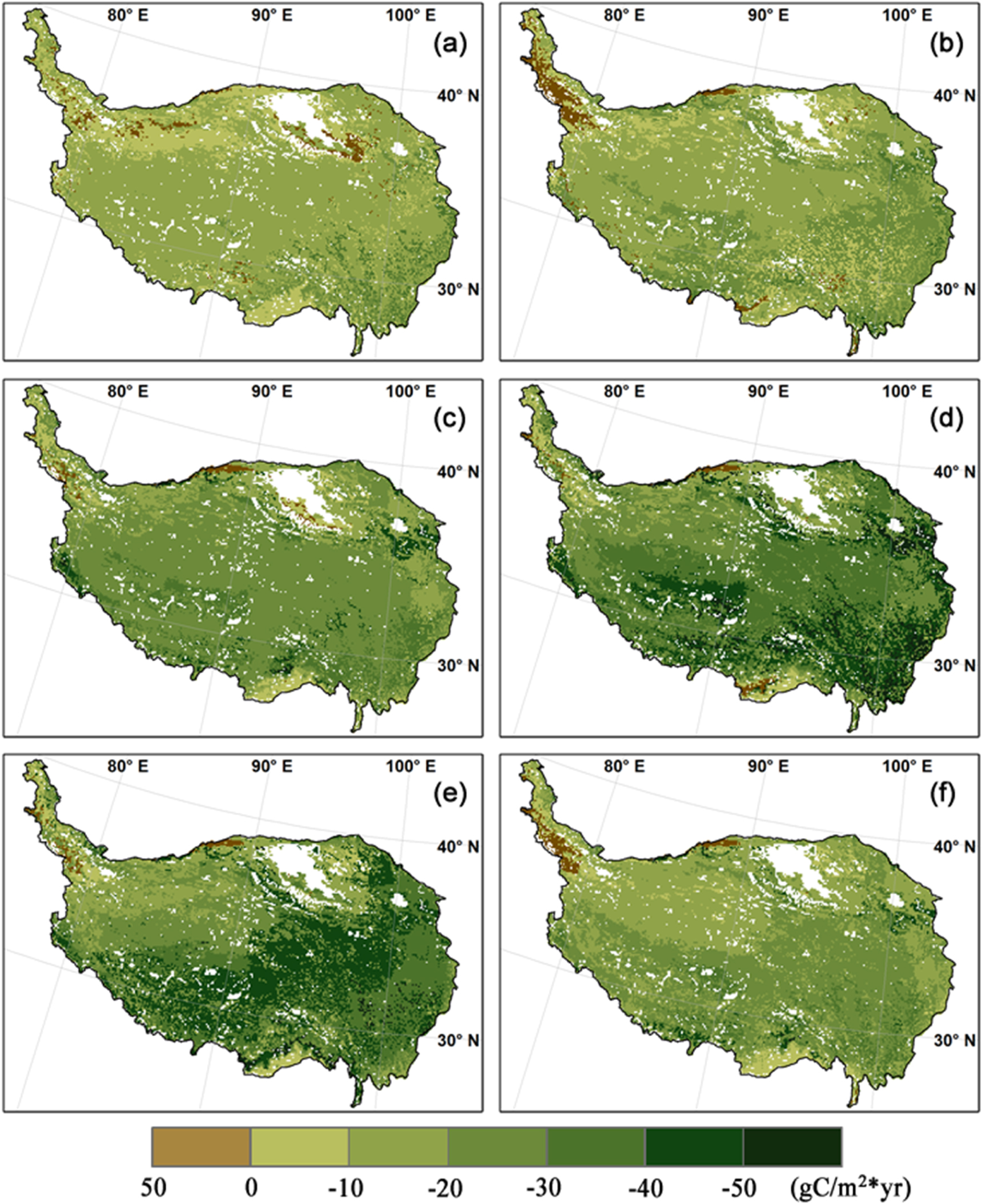
Spatial patterns of the decadal mean NME showed substantial variations over the QTP (figure 4). For the 2000s, net CH4 emissions simulated using reanalysis data were similar to the average of the RCP scenarios (figures 4(a) and (b)), with high net CH4 emissions occurred at Zoige wetland and in the southwest part of the QTP. Net CH4 sinks based on the two maps were comparable in magnitude, but high CH4 uptakes were found at the southern edge of the QTP in figure 4(a) rather than in the northeastern part in figure 4(b). At the end of the 21st century, the NME increased noticeably with respect to the magnitude over the QTP except for some southeastern parts (figures 1(c)–(f)). Among the models, RCP8.5 led to the strongest CH4 emissions in wetlands and the highest CH4 consumption in uplands. The difference in means between the RCP scenarios and the 2000s historical mean was statistically significant (α = 0.05) for most of the study area (figures S6(a)–(d)). Future climate change would strengthen the upland CH4 sink in the inner QTP, and substantially stimulate wetland CH4 emission in northeastern regions. For simulated NEP, most of the study region had a negative value (i.e. CO2 sink), with the magnitude up to −30 gC m−2 y−1 during the 2000s (figures 5(a) and (b)). The patterns were comparable with contemporary estimation for alpine grasslands by Zhuang et al (2010) and Piao et al (2012). Strong CO2 sinks occurred in the southeast of the QTP, where forest and shrubs were the dominant vegetation cover (figure 1(a)). CO2 sources accounted for a very limited portion of the total study area. Spatial patterns of NEP evolved substantially under future scenarios (figures 5(c)–(f)). The QTP became a uniform carbon sink under RCP2.6, indicating disproportional climate impacts on different ecosystem types. Increases in NEP were profound under two median scenarios, with differences statistically significant (α = 0.05) for most of the grassland (figures S6(f), (g)). Among these, the highest sink (up to 50 gC m−2 y−1) occurred in the forest ecosystem under RCP4.5 and in meadow regions under RCP6.0. NEP under RCP8.5 was distinctively lower than results under other scenarios and not statistically different from the historical 2000s mean (figure S6(h)), suggesting similar changes in the magnitude of NPP and RH for all ecosystem types.
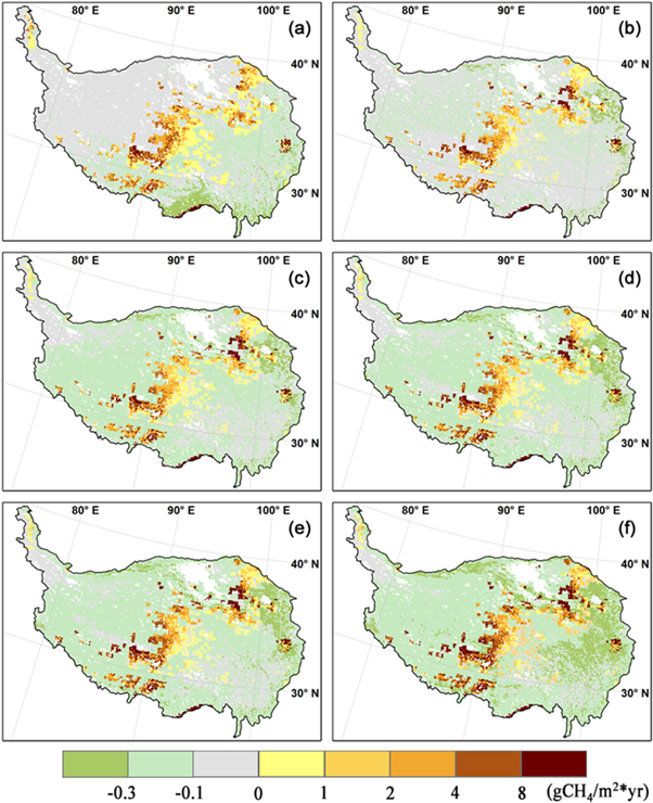
Figure 4. Spatial patterns of mean annual net methane exchange (NME) under different climate scenarios: (a) ECMWF reanalysis data for the 2000s; (b) mean CMIP5 RCPs from 2006–2010; (c) CMIP5 RCP2.6 for the 2090s; (d) CMIP5 RCP4.5 for the 2090s; (e) CMIP5 RCP6.0 for the 2090s; (f) CMIP5 RCP8.5 for the 2090s. Positive values indicate net emissions.
Download figure:
Standard image High-resolution image
Figure 5. Spatial patterns of mean annual net ecosystem production (NEP) under different climate scenarios: (a) ECMWF reanalysis data for the 2000s; (b) mean CMIP5 RCPs from 2006–2010; (c) CMIP5 RCP2.6 for the 2090s; (d) CMIP5 RCP4.5 for the 2090s; (e) CMIP5 RCP6.0 for the 2090s; (f) CMIP5 RCP8.5 for the 2090s. Negative values indicate carbon sinks.
Download figure:
Standard image High-resolution image3.3. Regional GHG budget
Our estimate of the total CH4 emissions from natural wetland over the QTP was 0.95 Tg CH4 y−1 during the 2000s, which was within the estimation range of 0.13–2.47 Tg CH4 y−1 from several other studies (table 3). The high variation among different estimates was mainly due to the uncertainty in wetland area estimates. Total CH4 consumption from those upland soils were 0.19 Tg CH4 y−1 (i.e. 20% of the regional CH4 emissions) for the 2000s, and increased slower than emissions under future scenarios (table 4), indicating that the QTP was likely to be a stronger CH4 source in the 21st century. The simulated regional NEP of  Tg C y−1 for the period 2006–2011 was lower than those for other modeling studies covering similar regions (Zhuang et al 2010, Piao et al 2012), but higher than that of Yi et al (2014). The near neutral properties of the historical NEP (also see figure 3(b)) were consistent with the results of Fang et al (2010), who found that soil C stock in China's grassland did not show a significant change during the past two decades. Future NEP increased under all RCP scenarios (table 4). Counter-intuitively, higher increases in NEP occurred under RCP4.5 and RCP6.0 instead of the warmest and wettest RCP8.5, indicating that carbon accumulation was more likely favored with modest warming and wetting.
Table 3. Existing estimates of CH4 emissions from wetland and alpine plant communities on the Qinghai-Tibetan Plateau.
| Wetland Area | Total | ||||
|---|---|---|---|---|---|
| Methods | Spatial Domain | Period | (×104 km2) | (Tg CH4 y−1) | Source |
| Inventory | Freshwater wetlands | 1996–1997 | 18.8 | 0.7–0.9 | Jin et al 1999 |
| Inventory | Natural wetlandsa | 2001–2002 | 5.52 | 0.56 | Ding and Cai 2007 |
| Inventory | Alpine meadow | 2003–2006 | 87.5 | 0.13 | Cao et al 2008 |
| Meta-Analysis | Natural wetlands | 1.49 | Chen et al 2013 | ||
| Meta-Analysis | Natural wetlands | 3.76 | 1.04 | Zhang and Jiang 2014 | |
| TEM | Natural wetlands | 1995–2005 | 11.5 | 2.47 | Xu et al 2010 |
| Coupled-TEM | Natural wetlands | 2001–2011 | 13.4 | 0.95 | This study |
aNatural wetlands include peatlands, freshwater marshes, salt marshes and swamps.
Table 4. Decadal mean of regional greenhouse gas budget.
| 2000s | 2050s | 2090s | ||
|---|---|---|---|---|
| ECMWF | 0.95 | |||
| RCP2.6 | 0.99 | 1.14 | 1.13 | |
| CH4 Emission | RCP4.5 | 0.97 | 1.18 | 1.28 |
| (Tg CH4 y−1) | RCP6.0 | 1.00 | 1.17 | 1.42 |
| RCP8.5 | 0.99 | 1.27 | 1.68 | |
| ECMWF | −0.19a | |||
| RCP2.6 | −0.20 | −0.23 | −0.23 | |
| CH4 Consumption | RCP4.5 | −0.19 | −0.24 | −0.25 |
| (Tg CH4 y−1) | RCP6.0 | −0.20 | −0.23 | −0.27 |
| RCP8.5 | −0.20 | −0.25 | −0.31 | |
| ECMWF | −10.22 | |||
| RCP2.6 | −18.08 | −33.44 | −37.01 | |
| NEP (Tg C y−1) | RCP4.5 | −23.03 | −38.96 | −45.76 |
| RCP6.0 | −20.92 | −30.27 | −41.67 | |
| RCP8.5 | −18.91 | −35.66 | −26.95 |
Instantaneous radiative forcing due to net CH4 emission and net CO2 sequestration since 1979 increased to a plateau during the 1990s, dropped to zero around the 2010 s, and decreased almost linearly afterwards (figure 6(a)). Therefore, climate change in the 21st century is likely to trigger negative feedback (cooling) in the climate system. Among these, the fastest decreased rate occurred under RCP4.5, indicating that this moderate climate warming scenario stimulated vegetation production much more than the methanogenesis process. A seemingly level-off trend after the 2080s was identified for the RCP8.5 scenario, most likely because of declining NEP (figure 3(b)). Cumulative radiative forcing was positive until the 2030s, and become negative in an accelerated manner (figure 6(b)). Thus, the cumulative GHG fluxes from the QTP will exert a slight warming effect on the climate system until the 2030s, but an increasingly stronger cooling effect thereafter. The tipping point was 50 years after the reference zero time point, roughly the time required for nearly complete removal of the initial CH4 perturbation input. At the end of the 21st century, cumulative mean radiative forcing was between −0.25 and −0.35 W m−2, depending on different RCP scenarios. Overall, our results show that given a sustained CH4 source and CO2 sink on the QTP, the net GHG warming effect will only peak after a few decades and will eventually contribute a more cooling effect to the climate system.

Figure 6. Instantaneous (a) and cumulative (b) radiative forcing for the period 1979–2100 calculated based on net CH4 and CO2 fluxes simulated with both historical (solid black line) and different RCP scenarios. Solid color lines are multi-model means, with shading representing one standard deviation.
Download figure:
Standard image High-resolution image
4. Discussion
4.1. Model optimization
Overall, our model calibration results were satisfactory, but a few tips should be mentioned when applying the global optimization method to complex system models with high parameter dimensions. Global optimization for problems without explicit analytic expressions of the objective function is challenging, because the algorithm must avoid being trapped by several local optima, while maintaining robustness in the presence of parameter interaction and non-convexity of the response surface, and having high efficiency in searching high dimensional space (Duan 2013). When applying the SCEM-UA, a tradeoff between goodness of fit and computational cost is still a problem for users.
The speed of algorithm convergence highly depends on the model structure and parameter interactions. In our case, major parameters evolved to a narrow range after 100 000 total iterations (figure S2). In contrast, the MDM optimization converged much slower despite the smaller number of parameters to be optimized. We argue that this is mainly due to the multi-scalar function method used to simulate CH4 production and oxidation. For instance, if scalars  and
and  are shaped with two parameters only, it is intuitive to imagine that many pairs of these two parameters can produce similar results, as long as they can adjust scalars
  and
and  in the opposite direction. Given that the scalar approach is extensively implemented in current ecosystem models (Zhuang et al 2004, 2010, Wania et al 2013, Zhu et al 2014), convergence criteria (such as the Gelman and Rubin diagnostic suggested by Vrugt et al (2003)) can hardly be reached for most parameters when calibrating these models.
On the other hand, sub-optimal is usually sufficient in practice. Increasing the sampling size from parameter space can push the posterior of the objective function to the high-end value (figure S2), but is by no means a guarantee of better model performance. Most likely, many behavioral parameter combinations with a similar capability of reproducing the observations can be found by a search conducted in the feasible parameter space (Vrugt et al 2003). As shown in our example, the top 500 parameter sets (whose values can differ) for either the STM or MDM produced close goodness-of-fit and small variations in simulations (figure 2), indicating that the benefits from additional searching are marginal.
4.2. Quantification of total GHG effect
To quantify and compare the net GHG effect of a sustained CH4 source and CO2 sink on the QTP, the total radiative forcing rather than the more widely known metrics of the GWP was computed in our study according to Frolking et al (2006). As a tool originally designed for evaluating and implementing policies to control multi-GHGs, the GWP is defined as the time-integrated radiative forcing due to a pulse emission of a given component, relative to a pulse emission of an equal mass of CO2 (IPCC, 2013). It has usually been integrated over a somewhat arbitrary time horizon of 20, 100 or 500 years, of which the choice of 100 years is most commonly adopted (e.g. CH4 is 28 times CO2 in terms of warming effect). Applying the GWP to biogeochemical cases could be problematic as GHG fluxes are often sustained and temporally dynamical from a long existing sink or source, even though many studies continue to use it because of its simplicity (e.g. Zhu et al 2013, Gatland et al 2014, Vanselow-Algan et al 2015). The method proposed by Frolking et al (2006) goes beyond the standard GWP approach such that (1) persistent emission or uptake of GHGs can be accounted for, and (2) the instantaneous radiative forcing for each year of simulation is quantified to allow a comparison of multiple gases in common units at any given time. Although the assumption of a near constant background atmosphere in Frolking's method is open to debate, and the decision on the appropriate pulse emission to consider (the new flux rate versus the change in the flux rate) could greatly change the results of the simulation, it appears a useful method in biogeochemical studies when accounting for the budget of multiple sustained GHG fluxes. Frolking's method has evolved with new findings in the atmospheric sciences. For example, the fraction of CO2 remaining in the atmosphere after a pulse input can be divided into four components (Joos et al 2013) instead of the original five-pool setting, and the multiplier of the indirect effect for CH4 is now 1.65 according to IPCC (2013). A test of these and other parameter changes is beyond the scope of this study.
4.3. Uncertainties and future work
This is the first study to quantify both CH4 emissions and net carbon exchanges on the QTP. However, the quantitative analysis is uncertain due to incomplete representation of physical and biogeochemical processes in the model (Bridgham et al 2013, Melton et al 2013, Bohn et al 2015), inaccurate model assumptions (Meng et al 2012), variations in the forcing climate data (Su et al 2013) and the extrapolation from site to regional scale. While progresses in model structures and mechanisms are usually slow and incremental, efforts to reducing data uncertainty are more feasible in a short period to improve model predictability.
First, seasonal and inter-annual dynamics of the wetland extent is critical to CH4 modeling. Synthetic aperture radar (SAR) is currently the first choice to delineate wetland distribution, such as the monthly distribution of surface water extent with ∼25 km sampling intervals used in this study (Papa et al 2010). However, optical remote sensing is highly sensitive to cloud or vegetation cover. Alternative data from passive and active microwave systems that will penetrate cloud and vegetation cover is favored (Schroeder et al 2010), but is currently unavailable over our study area. Some contemporary methane models, such as VIC-TEM and SDGVM, are capable of outputting dynamical wetland extent as an internal product (Hopcroft et al 2011, Lu and Zhuang 2012), but they tend to substantially overestimate wetland area (Melton et al 2013). In order to capture the seasonal flooding area, our study combined a static max potential inundation map and simulated water table depth to represent the wetland fluctuation. Improving the modeling abilities to capture wetland distribution and extent, especially the seasonality of water table dynamics, should be a research priority in the future (Zhu et al 2011).
The second uncertainty in quantifying CH4 emissions on a regional scale is from the spatial-scale extrapolation across highly heterogeneous but poorly mapped wetland complexes (Bridgham et al 2013). In this study, we only calibrated our model at one alpine wetland site by assuming that the remaining wetlands over the QTP have the same inert characteristics, but differ with climatic conditions. As a matter of fact, alpine wetlands on the QTP can be classified into peatlands, Marshes, and swamps, which have distinct characteristics in vegetation cover, hydrological processes, and soil history (Chen et al 2013). However, due to severe field experimental conditions, high quality observational data are mostly limited to the Lunhaizi wetland in Haibei Station (Hirota et al 2004, Yu et al 2013) and the Zoige wetland (Chen et al 2009, 2013). Field researchers should consider expanding field measurement footprints in the future, and data sharing with modelers is highly recommended.
Finally, much of the uncertainty in future projections is due to the poor agreement among CMIP5 GCMs under the RCP scenarios (figures S3, S4). The majority of the GCMs have cold biases of 1.1–2.5 °C in air temperature for the QTP, while they overestimate annual mean precipitation by 62%–183% (Su et al 2013). A multi-model ensemble approach, as was suggested in the IPCC AR5 report (IPCC, 2013), was used to configure the climatology uncertainty. While the statistical interpolation method used to generate fine resolution data is simple and computationally efficient (Wilby et al 1998), dynamical downscaling with regional climate models was more ideal to compensate for the shortage of coarse output from GCMs and to capture details of the complex surface properties of the QTP (Ji and Kang 2012). However, due to the high computational cost, dynamically downscaling climate data that cover representative GCMs under all RCP scenarios is generally not available to ecosystem modelers. A publicly accessible database like this would greatly benefit the research community in future studies.
5. Conclusions
Using a coupled biogeochemistry model framework, this study analyzed the carbon-based GHG dynamics over the QTP for the period 1979–2100. Our model simulations at the site level were able to closely match the field-observed soil temperature and CH4 flux after calibrating the model parameters using the SCEM-UA global optimization algorithm. Our study showed that the region currently acts as a CH4 source (emissions of 0.95 Tg CH4 y−1 and consumption of 0.19 Tg CH4 y−1) and a CO2 sink (14.1 Tg C y−1). In response to future climate change, the CH4 source and the CO2 sink strengthened, leading to an increasingly negative perturbation of radiative forcing. The spatial patterns and temporal trends of the NME and NEP highly depend on the RCP scenario. Climate-induced changes in the magnitude of the NME were statistically significant for most of the QTP, while spatial changes in the NEP were only significantly apparent under RCP4.5 and RCP6.0. The instantaneous radiative forcing impact is determined by persistent CO2 sequestration and recent (∼5 decades) CH4 emission. The cumulative GHG effect was a negative feedback (cooling) to the climate system at the end of the 21st century. Uncertainties in our model estimations can be reduced by including more explicit information on wetland distribution and classification, and more reliable future climate scenarios. Additional observational data from representative wetland ecosystems shall be collected to improve future quantification of these carbon-based GHGs.
Acknowledgments
This research is partially supported by funding to Q Z through an NSF project (DEB- #0919331), the NASA Land Use and Land Cover Change program (NASA-NNX09AI26G), the Department of Energy (DE-FG02-08ER64599), and the NSF Division of Information & Intelligent Systems (NSF-1028291). Jin-Sheng He and Weiming Song are supported by the National Basic Research Program of China (grant number 2014CB954004) and the National Natural Science Foundation of China (grant numbers 31270481 and 31025005).