
Abstract
This study presents an analysis of a three-dimensional unsteady two-temperature simulation of atmospheric pressure direct current electric arc inside a commercial cascaded-anode plasma spray torch; it coupled the arc model with the torch electrodes and used an open-source computational fluid dynamics software (code_saturne). The previously published models of plasma spray torch either deal with conventional plasma torches or assume local thermodynamic equilibrium in cascaded-anode plasma torches. The paper presents the computation of the two-temperature argon plasma properties, compares two enthalpy formulations that differ in association of the ionization part of enthalpy and finally demonstrates the influence of the radiation heat loss data by comparingthe results for two different literature sources. It is the first to compare different enthalpy formulations in the context of plasma torch and discuss the differences in terms of the enthalpy gains and losses. It also explains why an unphysical simulation artifact of electron temperature lower than the heavy species temperature can occur in simulated plasma flow. The solution, then, consists in associating the ionization part of enthalpy to electrons and selecting the appropriate source of the data of radiation heat loss. However, negligible thermal non-equilibrium persists even in the hot core of electric arc, which ensures that the heavy species are heated up by collisions with electrons. The flexibility of the open-source software allows all the necessary modifications and adjustments to achieve satisfactory simulation results. Thus, the paper could be considered as a manual for development of a plasma spray torch model.
Export citation and abstract BibTeX RIS

Original content from this work may be used under the terms of the Creative Commons Attribution 4.0 license. Any further distribution of this work must maintain attribution to the author(s) and the title of the work, journal citation and DOI.
1. Introduction
Reliable numerical models are often the only way to explore the thermodynamic and electromagnetic phenomena inside direct current (DC) plasma torches due to the small size of the torch cavity, high plasma luminosity and lack of any observation slits. Numerical simulations assuming departures from local thermodynamic equilibrium (LTE), especially close to the electrodes, are relevant so that two-temperature (2T) models should be applied to explore the processes inside a non-transferred arc DC plasma torch under atmospheric pressure.
Cascaded-anode plasma torches benefit from a limited displacement of the anode arc attachment on the anode wall and, thus, controlled arc length due to an electrically-neutral insert between the electrodes (Zhukov et al 1981). The latter makes the arc longer than in conventional plasma torches, which results in a higher voltage and higher enthalpy in the plasma flow. The cascaded anode makes it possible to achieve higher plasma enthalpy by an increase in arc voltage rather than arc current; it, thus, helps to keep the electrode erosion in reasonable limits, since the electrode weight loss due to arc erosion increases with an increase in arc current (Zhukov et al 1975, Lin and Wu 1995, Iwata and Shibuya 1998, Zhukov and Zasypkin 2007).
The continuum assumption is generally supposed to be valid in numerical simulations of DC plasma torches operated at atmospheric pressure. Therefore, the finite volume method that ensures the conservation of heat, mass and momentum in each control volume of the computational domain can be used. Also, the core of the plasma flow generated in such plasma torches can be considered as thermal plasma due to its high temperature, operation at atmospheric pressure and, thus, a sufficient collision rate between plasma species. This assumption allows considering one temperature for all the species in the computational control volumes. However, inside the torch at the arc periphery, the plasma species collision frequency is generally not high enough to compensate the imbalance in heat dissipation in electrons and heavy species that have significantly different mobility and diffusion rate. Below 8000 K, the collisions between electrons and heavy species are not sufficient to achieve LTE (Cram et al 1988). LTE requires an electron number density above 1021 m−3 (Griem criterion) (Griem 1964, Vacquié 2000), and plasma temperature to change slowly, smoothly and continuously compared to the equilibration time and equilibration length (Griem 1963).
The areas exposed to the cold plasma-forming gas flow or in contact with water-cooled metal parts might experience a rapid cooling of the heavy species while the electron heating by Joule power and thermal energy dissipation is so high, that the disequilibrium degree can reach a substantial level that cannot be described by only one temperature, even approximately. The consideration of thermal disequilibrium at the arc periphery is, thus, essential for the simulation of the cold boundary layer that develops on the nozzle wall. The simulated electric arc is non-transferred and has to make its way through this cold boundary layer. Therefore, the simulation of the departure from LTE inside the torch is required to understand the processes inside the plasma torch. The detailed analysis of the nonequilibrium phenomena presented in Trelles (2020) suggests to refer to such plasma flows as a quasi-thermal plasma flow.
The models of the cascaded-anode plasma torch which assume LTE in plasma include Molz et al (2007), Muggli et al (2007), Bobzin and Öte (2016), Zhukovskii et al (2020a, 2020b). The difference between LTE and thermal non-equilibrium in context of such plasma torch simulation was emphasized in Zhukovskii et al (2021).
The first step in considering the departure from LTE implies calculating two independent temperatures for electrons and heavy species, the so-called 2T approximation. A theoretical analysis of enthalpy formulation and radiation heat losses in 2T models is given in Freton et al (2012). The large variety of existing 2T models of transferred arcs includes Hsu and Pfender (1983), Haidar (1999), Freton et al (2012), Boselli et al (2013). Some of the existing models are time-dependent and three-dimensional like the model of a DC transferred arc twin torch presented in Colombo et al (2011). The simulation of a non-transferred arc is complicated by its curvature and requirements to consider time-dependence and three dimensions. Examples of 2T models of conventional plasma torches are described in details in Trelles et al (2007), Trelles and Modirkhazeni (2014), Modirkhazeni and Trelles (2018). In Trelles et al (2007) the importance and results of consideration of thermal non-equilibrium and its superiority over the LTE assumption were demonstrated in the context of conventional plasma torch simulation. It was demonstrated that the 2T model is more self-consistent and gives rise to better predictions of the arc dynamics. In Modirkhazeni and Trelles (2018) further attention is paid to the simulation of turbulent flow outside of the torch and difference between compressible and non-compressible models in an in-house code with the finite element method.
Further step in evolution of simulated non-equilibrium phenomena is consideration of chemical non-equilibrium, in other words simulation of plasma with composition assuming departure from the ionization equilibrium given by the Saha equation. Examples of chemical non-equilibrium models include the models of transferred arcs (Baeva et al 2016, 2019, Baeva 2017, Khrabry et al 2018) and plasma torches (Baeva and Uhrlandt 2011, Liang and Groll 2018, Sun et al 2020). The study (Liang and Groll 2018) of a conventional plasma torch with non-equilibrium plasma coupled with electrodes demonstrated the importance of taking into account the cathode sheath model in general and the cathode sheath voltage drop in particular for the accuracy of the torch model predictions. In addition, the chemical non-equilibrium modeling can be applied to induction plasma (Al-Mamun et al 2010). Simulation of the chemical non-equilibrium as in Baeva and Uhrlandt (2011) is beyond the scope of the present study and it is assumed that chemical equilibrium is reached in an atmospheric argon arc plasma operating at high current (500 A).
The studies (Liang and Groll 2018, Liang 2019, Liang and Trelles 2019) have a strong point in the advanced plasma-cathode coupling and taking into account the electrical conductivity of the collisionless cathode sheath. In Liang (2019) it was demonstrated that the consideration of the cathode sheath is important for accurate prediction of the cathode arc attachment.
The present study is focused on implementing a 2T 3D time-dependent model combined with the solid electrodes; it also compares several thermal configurations of the model in the context of a DC plasma torch. Following the terminology proposed in Trelles (2020), the model is intended to cover the kinetic nonequilibrium caused by microscopic imbalance in thermal energy. Meanwhile, the dissipative nonequilibrium caused by macroscopic instabilities, e.g. electron overheating instability, evaporation–ionization instability, multiple anode arc attachment (Yang and Heberlein 2007), and turbulence is beyond the scope of this study. Moreover, since the controlled arc length results in relatively low fluctuations in arc voltage, the pressure variations in the cathode cavity are expected to be low so that the model of a cascaded-anode plasma torch does not need to consider the compressibility (Rat and Coudert 2011) of plasma-forming gases.
The paper aims to demonstrate the way a 2T model can be developed in an open-source software and applied to a commercial cascaded-anode plasma torch in order to get a deep insight into the features of the arc inside the torch. The papers dealing with the thermal non-equilibrium in a cascaded-anode plasma torch are scarce, while further torch development requires more information about the arc in the torch.
Section 2 presents the simulated plasma torch, governing equations, plasma properties, boundary conditions and the way the 2T model was implemented in the software. Section 3 presents the computed distributions of electric current density, electron and heavy species temperatures and enthalpy balance in plasma for electrons and heavy species. Section 4 is intended to summarize the findings of the study.
2. Model description
The study deals with the commercial plasma spray torch SinplexPro™ manufactured by Oerlikon Metco shown in figure 1. The simulated plasma torch has a bore diameter of 9 mm; the distance between the cathode and anode is 26.6 mm. The cathode and anode liner colored in grey in figure 1 are included into the computational domain of the model. The cathode is made of sintered and machined Lanthanum(III) oxide-doped tungsten. The dopant plays the role of electron emitter due to its low work function and facilitates the machining of the electrode. The copper anode is protected by a tungsten liner that extends its life time due to the refractory properties of tungsten. The thickness of this liner is adjusted to optimize the thermal stress to which it is subjected and reduce, as much as possible, axial cracking and erosion (Molz and Hawley 2014).

Figure 1. Geometry configuration of the SinplexPro™ plasma torch. The tungsten parts of electrodes are colored in dark grey and the copper neutrodes and copper parts of electrodes in orange.
Download figure:
Standard image High-resolution imageThe model does not include the neutrodes in the computational domain; it considers them as a wall boundary condition and neglects the thin boron nitride rings that ensure the electrical insulation between each neutrode. In addition, it does not take into account the small circular cavities between the neutrodes intended to protect the ceramic rings from plasma radiation as they are believed to have no significant impact on the fluid dynamics. The validation of the 2T model against experimental data and its higher accuracy in terms of the anode arc attachment and arc voltage compared to the LTE model are presented in (Zhukovskii et al 2021).
2.1. Assumptions and governing equations
The simulation is implemented in an open-source computational fluid dynamics software code_saturne using the finite volume method. The computational domain includes the fluid area inside the torch from the gas inlet to the nozzle exit, outlet chamber and solid electrodes.
The plasma is assumed to be in chemical equilibrium and electrically neutral. The departure from chemical equilibrium that may appear in the periphery of the arc (Liang and Trelles 2019) is neglected in this study for the sake of computational cost efficiency. In addition, the plasma-forming gas in this study is pure argon, hence there is no demixing of the gas composition. The flow is assumed to be laminar, subsonic and weakly compressible. The laminar flow assumption is justified inside the plasma torch, while could be not valid outside of the torch (Pfender et al 1991, Modirkhazeni and Trelles 2018).
All the torch parts are assumed to be brand-new, perfectly aligned, without cracks and irregularities. Therefore, the model describes rather the initial phase of the torch operation. The electrical perturbations (ripple) produced by the power supply to the torch are neglected.
The governing equations employed in the model follow the pattern given in equation (1):
where  is the conserved property,
  the time,
  the flux of
  and
and  the net production or depletion rate. The first term on the left-hand side of equation (1) is the transient term and the second one is the advective-diffusive term. The system of the governing equations solved in the model is presented in table 1.
Table 1. System of governing equations.
Quantity
| Transient term | Advection and diffusion of 
| Source term 
|
|---|---|---|---|
| Mass |

|

| 0 |
| Momentum |

|
|
|
| Electron enthalpy |

|
|

|
| Heavy species enthalpy |

|
|

|
| Electric Potential | 0 |

| 0 |
| Magnetic vector potential | 0 |

|

|
In table 1
 is the plasma density,
  the magnetic field,
  the viscous stress tensor,
  the plasma pressure,
  the explicit and implicit momentum source terms used to cancel out the momentum inside the electrodes and control the gas injection angle,
  the magnetic vector potential which is used to derive the magnetic field as
  ,
,  the electric potential which is used to derive the electric field as
  , electric current density as
  , Lorentz force as
  , and Joule power as
  . Electric potential
  is a solved variable in code_saturne.
The solved thermal variables are the enthalpy of electrons  and enthalpy of heavy species
  , while all the plasma parameters depend on the corresponding temperatures
  and
and  . The continuum radiation
  was assigned to the electrons enthalpy equation following the suggestion of (Freton et al
2012). The radiation due to the absorbed and non-absorbed lines
was assigned to the electrons enthalpy equation following the suggestion of (Freton et al
2012). The radiation due to the absorbed and non-absorbed lines  is assigned to the heavy species.
  and
and  are electron and heavy species translational thermal conductivity.
  is the reactive thermal conductivity. The electron and heavy species specific heat
  and
and  depend on the formulation of enthalpy as described in the following section.
 is the exchange coefficient which, when multiplied by the difference of electron and heavy species temperatures, constitutes the energy exchange term between electrons and heavy species. However, if
  the exchange term is assumed to be zero. As it will be shown in the following, with some configurations of the 2T model, the predicted electron temperature can be lower than the heavy species temperature over a significant area of the simulated plasma flow, which was not observed experimentally (Murphy 2002). As it was shown in (Freton et al
2012), it is possible to mitigate the issue of
the exchange term is assumed to be zero. As it will be shown in the following, with some configurations of the 2T model, the predicted electron temperature can be lower than the heavy species temperature over a significant area of the simulated plasma flow, which was not observed experimentally (Murphy 2002). As it was shown in (Freton et al
2012), it is possible to mitigate the issue of  and make the results more plausible by allowing the exchange term to become negative, but the electron temperature will still be lower than the heavy species temperature, even though the difference will be much smaller. However, such approach would not have any theoretical ground. In addition, the problem in the enthalpy balance would persist. The present study is focused on developing a more accurate configuration of the 2T model of the plasma torch, hence the exchange term is not allowed to become negative.
Two different formulations of enthalpy are presented in the literature. The key difference is the association of the ionization component of enthalpy either to the heavy species as in equations (2) and (3) (Trelles et al 2007, Colombo et al 2011, Trelles and Modirkhazeni 2014, Liang and Groll 2018, Modirkhazeni and Trelles 2018), or to electrons as in equations (4) and (5) (Haidar 1999, Boselli et al 2013, Liang 2019, Liang and Trelles 2019). In the present study, the first formulation of enthalpy is referred to as 2T(I), and the second formulation as 2T(II) as follows:
where  is the formation energy of the ion
  .
.
The theoretical basis of the enthalpy formulation was explained in Freton et al (2012), where the authors insist that the ionization part of enthalpy should be associated to electrons because such formulation is derived from the Boltzmann equation. At first glance, the association of the ionization component of enthalpy to the electrons as it is done in the 2T(II) formulation might look unreasonable, since the free electrons do not have any physical connection to the ion. However, an electron needs to gain a sufficient amount of energy to overcome the attraction by the ion. Hence, the ionization energy associated to the electrons can be considered as the potential energy they carry. Such point of view reminds of the fact that the thermionic electrons emitted from the cathode surface carry away energy from the cathode resulting in its cooling by thermionic emission.
In addition, it was shown that these two enthalpy formulations can result in different temperature distributions of electrons and heavy species (Freton et al
2012). However, both options are widely used in plasma torch modeling. Therefore it is worth to compare them in the context of a cascaded-anode plasma torch and demonstrate which outcomes both of them bring about. Irrespective of the ratio  , it is expected that the assignation of the ionization part to the enthalpy of electrons or of heavy species will directly affect the amplitude of the gain and loss terms gathered in table 2 through the enthalpy value and its gradient. The contribution of the chemical reactions brought by ionization has indeed a major importance in the enthalpy as, for the same electron temperature, the electrons will store much more energy (kinetic and chemical) in the 2T(II) formulation than in the 2T(I) one.
Table 2. Terms of thermal equations segregated according to their sign, either positive, or negative, or both.
| Electrons | Heavy species | |
|---|---|---|
| Gains | 1. Joule power 
| 1. Exchange term |
| Losses | 1. Continuum radiation  2. Exchange term
| 1. Line radiation 
|
| Both gains and losses | 1. Convection  2. Enthalpy dissipation
  3. Enthalpy transport by electric current
| 1. Convection  2. Enthalpy dissipation
|
2.2. Data for the model
2.2.1. Plasma composition and thermodynamics properties.
Under the multi-temperature equilibrium assumption, the thermodynamic state of the system is fully described by the partition functions of each species. They comprise the translational, internal and reactional degrees of freedom of the entities in the plasma-forming gas and can be written as follows:
where  ,
,  ,
,  are respectively the translational, internal partition functions and formation energy of species i. The temperatures
  ,
,  and
and  are the translation temperature, temperature linked to the internal degree of freedom of heavy species and reaction temperature, respectively (Capitelli et al
2012).
are the translation temperature, temperature linked to the internal degree of freedom of heavy species and reaction temperature, respectively (Capitelli et al
2012).
In the case of a pure argon plasma, mainly the ionization reactions by electron impact have to be considered. In such conditions, it is assumed that the internal degrees of freedom of atoms and ions will be ruled by the electron temperature and ionization reactions as well, so that  ,
,  ,
,  .
.
Applying the maximization of the entropy to such a system gives rise to the 2-T Saha equation (Giordano 1998, Capitelli and Giordano 2002), often referred to as the van de Sanden formulation (Van De Sanden et al 1989). It follows that:
where  and
and  are respectively the electron number density and number desnity of heavy species with a charge number
  , and
, and  . The same notation is used for the internal partition functions of the heavy species
  .
.
The constants  ,
,  and
and  are the electron mass, Boltzmann constant and Planck constant, respectively.
  is the ionization energy lowering where
  is the Debye length and
  is the vacuum permittivity (Andre et al
1996).
is the vacuum permittivity (Andre et al
1996).
The internal partition functions are calculated from the NIST data (Kramida et al 2018) and their excited states number taken into account is limited by the ionization energy lowering. The latter is obtained by considering the Debye length involving the electrons only as recommended in (Murphy 2000).
The Dalton's law of partial pressures (8) and electrical neutrality assumption (9) are necessary to obtain the plasma composition:
where  and
and  are the total pressure and the number density of species
  , respectively.
The argon plasma composition is calculated up to 35,000 K at atmospheric pressure considering the electron, Ar, Ar+, Ar2+, Ar3+ and Ar4+ for different values of the disequilibrium degree  . For computational purposes, the data were generated for
  from 1 up to 25 with a step of 0.1 for the reasons given in the section about the implementation of the 2T model.
Figure 2 displays the number densities as function of the electron temperature for different values of  . The results are in good agreement with those obtained in Colombo et al (2008).

Figure 2. Pure argon plasma composition at atmospheric pressure for different values of the disequilibrium degree θ = Te /Th .
Download figure:
Standard image High-resolution imageIt has to be underlined that the widely used representation of figure 2, i.e. the electron temperature dependence of all number densities, is confusing because it is seen that the number densities of the major species (e, Ar, Ar+) increase as  increases while the total pressure is kept constant. The number densities of the heavy species are Th
-dependent: in a Th-representation their number densities are shifted to lower Th
temperatures as
increases while the total pressure is kept constant. The number densities of the heavy species are Th
-dependent: in a Th-representation their number densities are shifted to lower Th
temperatures as  increases. Note that the 2-T equilibrium constants of ionization reactions (right-hand side of equation (7)) are almost independent of
  even though the translation partition function of the heavy species
  are Th
-dependent. Consequently, if the reference temperature is Te
, the partial pressure of electrons increases as
are Th
-dependent. Consequently, if the reference temperature is Te
, the partial pressure of electrons increases as  increases at the expense of the partial pressure of the heavy species according to the total pressure conservation. At very low temperature,
  . At high Te
and
. At high Te
and  the electron number density tends to
  and becomes
  -independent as seen in figure 2 for
  .
.
Figure 3 depicts the electron enthalpy with the second formulation of enthalpy, referred to as 2T(II) in the previous section. The insert displays the low temperature values in a log-scale that is very useful for computational purposes. Only the 2T(II) enthalpy is shown because the other formulation (2T(I)) will lead to inconsistent results as shown in the next sections. As already known, the main contribution is due to the ionization terms highlighted by the changes in the slopes. For a given Te
, the electron enthalpy decreases with an increase of  due to the increase of the mass density conditioned by the increase of the number density of ions seen in figure 2.
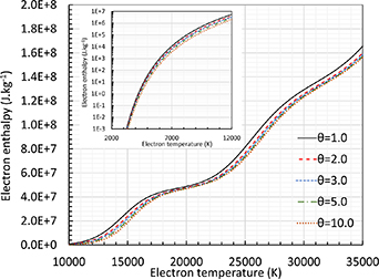
Figure 3. Electron enthalpy of pure argon at atmospheric pressure for different θ values according to the definition given by equation (4). Linear scale for high temperature range and logarithmic scale for low temperature range.
Download figure:
Standard image High-resolution imageThe last thermodynamic properties useful for the 2-T model is the specific heat derived from the specific enthalpy. Figure 4(a) displays a comparison of the specific heat with Colombo et al (2008) calculated as  ; a very good agreement is found between both calculations. However, we have adopted a different definition, i.e.
  and
and  . Figure 4(b) shows the electron temperature dependence of
  , derived from the 2T(II) enthalpy formulation, for different values of
  . The specific heat of heavy species in the 2T(II) formulation is almost constant, i.e.
  .
.

Figure 4. Specific heat of pure argon at atmospheric pressure for different θ values (a) comparison with (Colombo et al
2008) and (b) electron contribution according to the definition  .
.
Download figure:
Standard image High-resolution image2.2.2. Transport coefficients.
This section briefly displays the 2-T argon transport coefficients calculated for the model. The details of formulae used are not shown here but can be found for example in Colombo et al (2008) and references therein. A comparison of the equilibrium and 2-T calculations with previous published results is also carried out. The collision integrals  for species collisions in the argon plasma are calculated at the Te
temperature when a collision involves an electron and at Th
otherwise. The temperature dependence of the collision integrals (e-Ar, Ar-Ar, Ar-Arz+) are taken from Aubreton and Fauchais (1983). The collision integrals for charged species are calculated from the approach given by Mason et al (1967), Devoto (1973) considering the screened Coulomb potential involving the Debye length involving the electrons only.
for species collisions in the argon plasma are calculated at the Te
temperature when a collision involves an electron and at Th
otherwise. The temperature dependence of the collision integrals (e-Ar, Ar-Ar, Ar-Arz+) are taken from Aubreton and Fauchais (1983). The collision integrals for charged species are calculated from the approach given by Mason et al (1967), Devoto (1973) considering the screened Coulomb potential involving the Debye length involving the electrons only.
Figure 5 presents the electrical conductivity for different  values. A good agreement is found at equilibrium with Murphy (2000), Colombo et al (2008) and also for non-equilibrium conditions with Colombo et al (2008). Below roughly 12,000 K, it decreases when
  increases as shown in the insert. Actually, the plasma is dominated by the collisions between heavy species so that the collision integrals
  turn out to be higher as
  increases, hence the decrease of electrical conductivity. Above 12,000 K, the electrical conductivity follows the electron number density
  -dependence of figure 2. Figure 6 depicts the thermal conductivities, including the translational thermal conductivity of electrons and heavy species,
  and
and  respectively, and the reactive thermal conductivity
  . The viscosity is shown in figure 7. Again, a good agreement is found with (Murphy and Arundell 1994, Murphy 2000, Colombo et al
2008). The dependence of the coefficients
. The viscosity is shown in figure 7. Again, a good agreement is found with (Murphy and Arundell 1994, Murphy 2000, Colombo et al
2008). The dependence of the coefficients  on
on  is consistent with the electron number density. The coefficient
  decreases with
  because of the collision integrals
  . The viscosity has the same
  - dependence as
  .
.
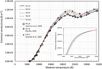
Figure 5. Electrical conductivity of pure argon at atmospheric pressure for different θ. Linear scale for full temperature range and logarithmic scale for low temperature range.
Download figure:
Standard image High-resolution image
Figure 6. Thermal conductivity of pure argon at atmospheric pressure for different θ values (a) translation contribution of electron and heavy species, (b) reactive thermal conductivity.
Download figure:
Standard image High-resolution image
Figure 7. Viscosity of pure argon at atmospheric pressure for different θ values.
Download figure:
Standard image High-resolution imageA good agreement is also found for  at equilibrium (Murphy and Arundell 1994). It has to be underlined that different approaches were published and discussed in the 2-T assumption, as for example in (Capitelli et al
2012) or (Santos et al
2019). It is beyond the scope of this paper to debate the effect of the different methods, which would require a close examination together with the methods of plasma composition calculation. Instead,
at equilibrium (Murphy and Arundell 1994). It has to be underlined that different approaches were published and discussed in the 2-T assumption, as for example in (Capitelli et al
2012) or (Santos et al
2019). It is beyond the scope of this paper to debate the effect of the different methods, which would require a close examination together with the methods of plasma composition calculation. Instead,  is calculated according to the method described in Bonnefoi and Fauchais (1983) and exhibits a decreasing evolution with
  as shown in figure 6(b).
2.2.3. Exchange coefficient.
The exchange coefficient is calculated with the equation (10) as in Trelles et al (2007), Freton et al (2012):
 is the elastic collision frequency between the electron and heavy species i and
  .
.  and
and  are the electron mean speed and average elastic cross section, respectively, calculated according to Freton et al (2012).
Figure 8 shows the exchange term  for different
  values and different scales. It is seen that
  increases with
  like the electron number density.
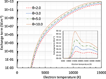
Figure 8. Exchange term of pure argon at atmospheric pressure for different θ values. Logarithmic scale for low temperature range and linear scale for high temperature range.
Download figure:
Standard image High-resolution image2.2.4. Radiative properties.
The energy conservation equations require the calculation of the divergence of the radiative flux which represents the net balance between the emission and absorption radiative processes. In the commonly-used approach of the net emission coefficient (NEC), the absorption coefficient, which encompasses all the continuum and lines contributions and includes the integration over all the spectrum wavelengths assuming the radiation isotropically emerges from an isothermal sphere of radius  (Lowke 1974, Liebermann and Lowke 1976). For reasons linked to the computational cost (Trelles and Modirkhazeni 2014) and availability of ready-to-use NEC data as a function of temperature, the NEC approach is used in many models (Colombo et al
2011, Boselli et al
2013, Liang and Groll 2018, Modirkhazeni and Trelles 2018, Liang 2019, Liang and Trelles 2019). It has to be noted that the NEC coefficient cannot consider the absorption in the fringes of the arc or in the cold gas surrounding the arc, which would bring about a negative divergence of the radiative flux in these low temperature regions (Kovitya and Lowke 1985, Randrianandraina et al
2011). In other models (Trelles et al
2007, Baeva et al
2016, 2019, Baeva 2017), the radiation power is estimated by means of the Beulens' et al formula (1991) that gives a dependence on the electron number density.
(Lowke 1974, Liebermann and Lowke 1976). For reasons linked to the computational cost (Trelles and Modirkhazeni 2014) and availability of ready-to-use NEC data as a function of temperature, the NEC approach is used in many models (Colombo et al
2011, Boselli et al
2013, Liang and Groll 2018, Modirkhazeni and Trelles 2018, Liang 2019, Liang and Trelles 2019). It has to be noted that the NEC coefficient cannot consider the absorption in the fringes of the arc or in the cold gas surrounding the arc, which would bring about a negative divergence of the radiative flux in these low temperature regions (Kovitya and Lowke 1985, Randrianandraina et al
2011). In other models (Trelles et al
2007, Baeva et al
2016, 2019, Baeva 2017), the radiation power is estimated by means of the Beulens' et al formula (1991) that gives a dependence on the electron number density.
The NEC given by Erraki (1999), Freton et al (2012) that considers the contributions of continuum and lines radiation of argon where the self-absorption of lines is taken into account in this paper. Figure 9 displays the NEC of argon at atmospheric pressure and at LTE. It shows that the absorption has to be considered when comparing  (Menart and Malik 2002) and
  (Erraki 1999). Figure 9 also shows the continuum NEC from (Erraki 1999). The lines emission contribution (including the self-absorption lines), NEC (total)—NEC (continuum), is important especially at high temperatures.

Figure 9. Net emission coefficient of pure argon.
Download figure:
Standard image High-resolution imageNote that Beulens et al (1991) give a valid approximation only up to 15,000 K for the total and continuum NEC as shown in figure 9 by the extrapolation of the Beulens' et al formula obtained with the plasma composition calculated up to 35,000 K. The approximation does not consider any absorption which does not hold at high temperature where radiation losses are the highest. However, this approximation is easy to handle for different  since it depends on the electron number densities. However, it has to be underlined that the radiation losses are dominant for high current arcs leading to high temperatures and also to thermal equilibrium that is why one can assume the radiation losses are independent of
  at least in the NEC approximation.
Moreover, the radiation power is split between the energy equations of electron and heavy species assuming that the free-free and free-bound transitions leading to radiative emission correspond to electron energy loss mechanisms. The bound-bound transitions produce radiation losses from the heavy species (Freton et al
2012). The last statement can be questionable and suggests that the electron kinetic energy is weakly affected by inelastic collisions populating the excited states of heavy species. We suppose that only the tail of the electron distribution function may have departure from the Maxwellian distribution which weakly affect the mean electron kinetic energy electrons for  temperatures below 35,000 K. Consequently, as also supposed by Freton et al (2012), the radiation losses due to the continuum transitions are ascribed to the electron energy equation while the line transitions are attributed to the heavy species equations.
The effect of the radiative properties (Beulens et al 1991, Erraki 1999) on modeling results will be shown in the following.
2.3. Boundary conditions
The boundary conditions and the computational domain are shown in figure 10. The model requires boundary conditions for all of the solved variables: electron and heavy species enthalpy, velocity, electric potential and magnetic vector potential. The approach of the recalculation of the boundary condition for the magnetic vector potential according to the Biot and Savart law is described in Freton et al (2011), Zhukovskii et al (2020b).

Figure 10. Computational domain and boundary conditions. Lines over which the analysis is done: 1 is the torch axis, 2 is the line across the torch channel 1 mm downstream of the cathode tip, 3 is the line across the nozzle exit.
Download figure:
Standard image High-resolution imageThe boundary condition for electric potential consists in imposed values of electric potential on the external surfaces of the solid electrodes (colored in grey in figure 10), zero-flux boundary condition on the other boundaries of the computational domain and continuous coupling of electric potential at the plasma-electrode interface. The continuous coupling in this case is a simplification, because the cathode and anode sheaths are not considered in this study. The electric potential on the external surface of the anode is assumed to be zero, as shown in figure 10. Hence, the electric potential imposed on the external surface of the cathode is equal to the negative recomputed voltage. A zero-flux of electric potential was assumed on the surface of the neutrodes inserted between the cathode and anode. In other words, the neutrodes are assumed electrically insulated. Therefore, the electric arc cannot connect to the neutrodes.
2.3.1. Thermal boundary conditions.
For the sake of clarity, the thermal boundary conditions are expressed in terms of temperature. In fact, in the model, the values imposed in the Dirichlet boundary conditions are the values of enthalpies, taken from the lookup tables of the plasma properties.
The only boundary where the electron temperature is explicitly imposed (Dirichlet boundary condition) is the inlet. The electron temperature at the inlet is assumed to be 1950 K. Below this temperature, the electron number density is too low resulting in much less than one electron per fluid cell, which makes the concepts of Maxwellian distribution and electron temperature inapplicable. An artificial increase in the electron number density at low temperatures, which is used in some 2T arc simulations (Trelles et al
2007, Freton et al
2012) to equalize the electron and heavy species temperature in the cold periphery, does not change the distributions of the arc plasma properties in our model while it produces unwanted fluctuations in the exchange term and predicted electron temperature. The heavy species temperature at the inlet is assumed to be 300 K. Thus, the disequilibrium degree  at the inlet is 6.5.
The electron temperature on the other boundaries has a zero-flux boundary condition. Zero flux of electron temperature on the neutrode wall is assumed due to the low sensitivity of the model to the imposed boundary condition. Even  of 300 K imposed on the neutrode wall results in noticeable changes of the electron temperature only in the boundary cells. This is because the simulated electron enthalpy balance in the periphery of the arc is dominated mostly by the Joule power, exchange term and, to a much lesser extent, by convection and dissipation. The zero-flux boundary condition for electron temperature on the electrode surface in this case is a simplification while in general the electron temperature on the electrode-plasma interface should be defined by a sheath model, which is omitted in the present study. Due to the lack of cathode sheath, the electron temperature in plasma is not coupled with the cathode temperature and does not affect the thermionic emission on the cathode surface.
The heavy species temperature on the surface of the neutrodes is assumed to be 500 K between the cathode tip and anode due to the heating of the neutrodes by the plasma radiation and 300 K upstream from the cathode tip where the injected gas is still cold. The model has little sensitivity to the exact value of the thermal boundary condition on the neutrode surface between the electrodes. An increase of the assumed neutrode temperature by 100 K in the model results in barely noticeable changes in other model indicators. Since the model does not include the copper neutrodes, the neutrode surface temperature of 500 K is merely an assumption needed to take into consideration the neutrode heating by plasma radiation. In the real SinplexPro plasma torch, a water-cooling circuit ensures a constant wall temperature.
2.3.2. Inlet boundary condition.
The plasma-forming gas is injected through 24 small spots behind the cathode as shown in figure 10. It is intended to imitate the gas injection through the 24 holes of the gas injector ring of the actual torch. The gas injection angle is set at 25°, which is controlled through the momentum source term at the boundary cells. The injection through small holes increases the angular momentum and, thus, intensifies the flow swirling. The velocity at the boundary condition is controlled in order to maintain the gas flow rate, which in this study was set at 60 normal liters per minute (NLPM).
2.3.3. Voltage scaling algorithm and control of current intensity.
The voltage  applied on the external surface of the cathode as boundary condition is recomputed after each time step in the model in order to maintain the imposed electric current intensity through the plasma (Électricité de France R&D 2017, Zhukovskii et al
2020b). As a part of the voltage scaling algorithm the total Joule power in the model from the previous time step is computed and compared with the product of the imposed current intensity (I) and voltage (V) imposed at the previous time step. If the total Joule power is higher than the product I·V, the voltage is decreased proportionally, and vice versa. In order to avoid detrimental fluctuations at the beginning of the simulation, when all the parameters change a lot from one time step to the other, the increment of the recomputed voltage is limited by 10% per time step. The time-evolution of the arc voltage computed this way is shown in figure 11. A similar method with the recalculation of the imposed voltage was employed in Baeva and Uhrlandt (2011).
applied on the external surface of the cathode as boundary condition is recomputed after each time step in the model in order to maintain the imposed electric current intensity through the plasma (Électricité de France R&D 2017, Zhukovskii et al
2020b). As a part of the voltage scaling algorithm the total Joule power in the model from the previous time step is computed and compared with the product of the imposed current intensity (I) and voltage (V) imposed at the previous time step. If the total Joule power is higher than the product I·V, the voltage is decreased proportionally, and vice versa. In order to avoid detrimental fluctuations at the beginning of the simulation, when all the parameters change a lot from one time step to the other, the increment of the recomputed voltage is limited by 10% per time step. The time-evolution of the arc voltage computed this way is shown in figure 11. A similar method with the recalculation of the imposed voltage was employed in Baeva and Uhrlandt (2011).
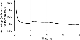
Figure 11. Time-evolution of the simulated arc voltage computed through the voltage scaling algorithm.
Download figure:
Standard image High-resolution image2.4. Implementation of the 2-T model
2.4.1. Software adaptation to 2-T model.
For this study, the open-source software code_saturne was adapted for the 2-T modeling of electric arc. For that an extra user scalar was added with its own diffusivity and source terms. The user-added scalar was solved by the same solver as the default thermal variable. The first step in development of the 2-T model was similar to the one described in Freton et al (2012): default and user-added thermal equations are duplicated as LTE, in order to verify that these two equations are numerically identical. Both thermal scalars, default and user-defined, are the same in the way their initialization, boundary conditions and source terms can be treated in the user subroutines.
The thermal variable in code_saturne by default is the enthalpy because it is convenient for the computation of the energy balance: the thermal source terms and thermal flux, which are usually expressed in terms of energy, can be used as they are. In addition, the use of enthalpy as the thermal variable allows to simulate the phase transition in the cells of the electrodes included into the computational domain. During the phase transition from solid to liquid the energy accumulated in the heated cells of the electrode increases, while the temperature remains the same. Therefore, the temperature cannot be used to capture this process. In the 2-T model, the thermal equations solved inside the electrodes are identical for the default thermal variable and the used-added one.
However, when enthalpy is used as the thermal variable, a problem arises: all the plasma properties are defined as functions of temperature and not of enthalpy. These properties are usually stored in a lookup table, which associates the precalculated values of plasma properties to each value of some certain set of temperature values. Therefore, in order to calculate the plasma properties for a given cell, the temperature is first needed. In the LTE model, the translation of the enthalpy to temperature is done using a simple lookup table with one column for temperature and one column for enthalpy. Meanwhile, the 2-T model solves the enthalpy of electrons  and enthalpy of heavy species
  , which must be translated into the temperature of electrons and temperature of heavy species. The solution of this problem is not as straightforward as in the LTE case, since both enthalpies are functions of both temperatures. In order to solve this issue a set of disequilibrium degrees
  is selected prior the running of simulation. The set of
  must be fine enough to guarantee the smooth transitions of all the properties from one
  to another. For each
  a lookup table with plasma properties as functions of electron temperature is built. Thus, the number of elements in the set
  is equal to the number of lookup tables used in the model. The interpolation between the values of
  is not employed in order to optimize the computational cost of the plasma properties recalculation at each time step for each cell.
In order to obtain the electron and heavy species temperatures of a given cell for calculation of the plasma properties the following procedure is performed. The enthalpies  and
and  are taken either from the previous time step or from the initialization values for the first time step at the start of the model run. For each value
  from the set
  a simple translation
  and
and  is done. Following that, the initial set
  is compared with the obtained set of ratios
  . Some obtained ratios of temperatures are higher than the initial
  , some are lower. The closest obtained ratio
  to the initial
  is selected as the best fit. The best fit
  is assigned to the given cell and, using the obtained
  , all the other plasma properties are calculated for the given cell.
Each simulation instance starts with the assignment of the initial values of all the solved variables. After the variable initialization, the following key stages are repeated during each time step in the developed 2-T model in code_caturne:
- (a)Translation of enthalpies to temperatures:
 .
. - (b)Update of the plasma properties as functions of and for each plasma cell (density, thermal and electrical conductivities, viscosity, exchange term, radiation heat loss, specific heat).
- (c)Assignment of the boundary conditions for all the solved variables. The boundary condition for the magnetic vector potential is recomputed once per 2 time steps during the initial 30 time steps and once per 100 time steps afterwards.
- (d)Assignment of the source terms for velocity: user source terms and Lorentz force.
- (e)Solution of the equations of mass and momentum conservation, computation of pressure.
- (f)Assignment of the source terms for the electron enthalpy: exchange term, Joule power, heat transport by electric current, continuum radiation.
- (g)Solution of the equation of the electron enthalpy.
- (h)Solution of the equation of electric potential
- (i)* Recalculation of the electric field, electric current density and Joule power
- (j)* Voltage scaling algorithm.
- (k)Solution of the equation of the magnetic vector potential
- (l)* Recalculation of the magnetic field and Lorentz force .
- (m)Assignment of the source terms for the heavy species enthalpy: exchange term, line radiation.
- (n)Solution of the equation of the heavy species enthalpy.
- (o)Output of the computed values and start of the following iteration.


The computational time cost of the 2-T model is not significantly higher than the time of the LTE model used in this laboratory: 2 h 45 min per 1000 time steps for the 2-T model against 2 h per 1000 time steps for the LTE model. The additional computational time is mostly associated to the extra solved scalar and translation of enthalpies to temperatures. On the other hand, due to considered thermal non-equilibrium and hence lower gradient of electron temperature compared to the gradient of LTE temperature, the electrical conductivity of plasma along the entire path of electric current from the cathode to the anode is much smoother. Thus, the average number of iterations necessary for the solution of the equation for the electric potential decreases from 12 in the LTE model down to 2 in the 2-T model. After the right initialization parameters are found and all the local instabilities are eliminated, the 2-T model becomes more numerically stable than the LTE model.
2.4.2. Electrodes inclusion in the computational domain.
The velocity inside the electrodes is zeroed through the momentum source terms as suggested in Patankar (1980).
The anode and cathode sheaths are beyond the scope of this study. Thus, the cathode and anode voltage drops are assumed to be constant in time and uniform over the whole surface of each electrode. It is important to mention that, when the cathode sheath is considered, the predicted cathode arc attachment tends to be more realistic (Liang 2019). The cathode and anode sheath voltage drops are assumed to be 10 V and 0 V respectively.
The electrode heating by the electric current is implemented as described in Zhukovskii et al (2021). For that purpose, the heavy species enthalpy field is coupled with the enthalpy of the electrode by the continuity of corresponding temperatures. The continuous transition of the plasma heavy species temperature to the electrode temperature in this case is a simplification, since the model neglects the anode and cathode sheath. Thus, the enthalpy balance at the electrode surface is rather approximate and requires further development.
3. Results and discussion
In the simulation results, all the distributions converge to a steady state after 50,000 time steps or 5 ms of the simulated time even though the model includes transient processes. This includes the plasma swirling, electric current density and temperature. An example of the convergence of the simulation to the steady state is shown in figure 11, which represents the time-evolution of arc voltage. All the presented distributions and curves are given for a simulated time of 5 ms. In the following, a comparison of the results will be made along the different lines defined in figure 10 allowing us to track the evolution of plasma properties along the torch channel.
3.1. Enthalpy formulation
When comparing the electric current density streamlines for both formulations 2T(I) and 2T(II) with 500 A and 60 NLPM of pure argon, we can notice that the predicted electric arc is axisymmetric with a rather diffuse anode arc attachment as it can be seen in figure 12. The highest value of the electric current density is found at the cathodic jet, where the arc is constricted by the surrounding cold gas flow.

Figure 12. Electric current density streamlines with 500 A, 2T(I) and 2T(II) formulations of enthalpy.
Download figure:
Standard image High-resolution imageA comparison of electric current density profiles across the torch channel along the line 2, i.e. close to the cathode in figure 10, is demonstrated in figure 13. The cathode arc attachment is a little more constricted with the 2T(I) formulation as the current density is lower in the periphery of the arc and higher in the arc core for R = 0.5–1.5 mm.
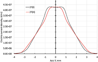
Figure 13. Electric current density profiles across the torch channel (line 2) with 500 A, 2T(I) and 2T(II) formulations.
Download figure:
Standard image High-resolution imageDue to the high electric current density at the cathode arc attachment, the highest electron temperature around 24,000 K is found in the cathodic jet as it can be seen in figure 14. The first difference between the 2T(I) and 2T(II) formulations along the line 1 is the higher electron temperature in the cathodic jet and lower temperature at the nozzle exit with the 2T(I) formulation as seen in figure 15. In addition, for a radius lower than 2 mm, the electric current density with the 2T(I) formulation following the line 2 exhibits a wider profile resulting also in a wider electron temperature profile as confirmed by figure 16. However, the electron temperature in the cathodic jet with the 2T(I) formulation is higher only for a radius lower than 2 mm.
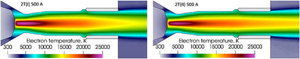
Figure 14. Electron temperature with 500 A, 2T(I) and 2T(II) formulations of enthalpy and radiation loss data from Erraki (1999). Time step is 10−8 s with 2T(I) and 10−7 s with 2T(II).
Download figure:
Standard image High-resolution image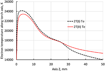
Figure 15. Axial electron temperature profiles along the torch axis (line 1) with 500 A, 2T(I) and 2T(II) formulation and radiation loss data from Erraki (1999).
Download figure:
Standard image High-resolution image
Figure 16. Radial electron temperature profiles across the torch channel (line 2) with 500 A, 2T(I) and 2T(II) formulations and radiation loss data from Erraki (1999).
Download figure:
Standard image High-resolution imageIt is worth underlining that the axial electron enthalpy profiles of 2T(I) and 2T(II) formulations exhibit different evolutions from temperatures as seen in figure 17. The electron enthalpy of 2T(II) formulation is much higher because it contains the ionization contribution of enthalpy. Figure 3 depicts the temperature dependence of the electron enthalpy of the 2T(II) formulation. Two consecutive steep increases of enthalpy can be observed, mainly due to respectively the first and second ionization of Ar atoms meanwhile the temperature changes to a lesser extent. Hence, the 2T(II) electron enthalpy formulation can result in an electron temperature lower than the 2T(I) one since, without the stored chemical energy, the same enthalpy will bring about a much higher electron temperature.
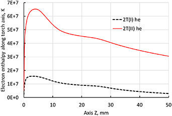
Figure 17. Axial electron enthalpy profiles along the torch axis (line 1) with 500 A, 2T(I) and 2T(II) formulation and radiation loss data from Erraki (1999).
Download figure:
Standard image High-resolution imageThe heavy species temperature at the nozzle exit is higher with the 2T(I) formulation than with the 2T(II) formulation as seen in figure 19. The comparison of figures 14 and 19 shows that the heavy species temperature on the torch axis is obviously higher than the electron temperature at the nozzle exit and in the outside domain with the 2T(I) formulation. Meanwhile, the electron temperature with the 2T(II) formulation does not seem to be lower than the heavy species temperature.
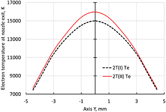
Figure 18. Radial electron temperature profiles at the nozzle exit (line 3) with 500 A, 2T(I) and 2T(II) formulations and radiation loss data from Erraki (1999).
Download figure:
Standard image High-resolution image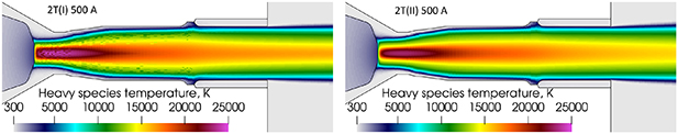
Figure 19. Heavy species temperature with 500 A, 2T(I) and 2T(II) formulations of enthalpy and radiation loss data from Erraki (1999). Time step is 10−8 s with 2T(I) and 10−7 s with 2T(II).
Download figure:
Standard image High-resolution imageThe distribution of the disequilibrium degree  is shown in figure 20. The regions with the electron temperature lower than the heavy species temperature (
 ), are colored in shades of blue. The 2T(I) formulation results in a large region with
  , which is considered to be unphysical for a 2-T model (Freton et al
2012) while, the 2T(II) formulation results in
, which is considered to be unphysical for a 2-T model (Freton et al
2012) while, the 2T(II) formulation results in  strictly larger than unity. The disequilibrium degree in the 2T(II) formulation goes as low as 1.001 in some areas, but never reaches exactly 1.0.
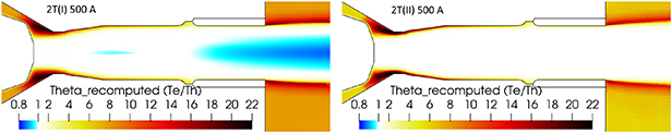
Figure 20. Disequilibrium degree θ = Te /Th with 500 A, 2T(I) and 2T(II) formulations of enthalpy and radiation loss data from Erraki (1999). The blue areas correspond to θ < 1. Time step is 10−8 s with 2T(I) and 10−7 s with 2T(II).
Download figure:
Standard image High-resolution imageAnother important point to note about the 2T(I) formulation is the spatial fluctuations of the heavy species temperature with a current intensity of 500 A. The ripple of the heavy species temperature can be seen as noise in figure 19. In fact, these spatial fluctuations in the 2T(I) formulation make it necessary to decrease the time step from the default one of 0.1 μs down to 10 ns. The 2T(I) formulation with the default time step of 0.1 μs has a too unstable behavior and worse convergence due to the thermal instabilities and fluctuations of Joule power and exchange term in the cathode vicinity. The tenfold decrease in the time step reduces the fluctuations but does not eliminate them. In addition, the 2T(I) formulation has a ten times higher computational cost per simulated unit time compared to the 2T(II) formulation due to the requirement of a smaller time step. Meanwhile, the 2T(II) formulation works well with the default time step and does not seem to produce spatial fluctuations of the heavy species temperature.
3.2. Comparison of different enthalpy source terms
In the previous section, it was observed that the electron temperature is higher for the 2T(I) formulation than for the 2T(II) one following the line 2 (figure 10) and on the torch axis inside the torch. In both cases, LTE is reached. At the nozzle exit following the line 3 (figure 10), the situation is inversed, i.e. the electron temperature for the 2T(II) model is higher as seen in figure 18. This is attributed to the ionization enthalpy associated with the electrons or heavy species. Moreover, an important issue of a 2T(I) enthalpy formulation is the formation of areas with the electron temperature lower than the heavy species temperature or  , which was not observed experimentally in thermal plasmas (Murphy 2002). In order to better understand the simulated process and why the
  areas appear, this section is dedicated to an analysis of the enthalpy balance made along the line 1 shown in figure 10.
The thermal configuration of each area in the torch channel is always the matter of a balance between enthalpy gains and losses in electrons and heavy species. Different areas inside the torch might have a striking difference in the proportions and order of magnitude of each thermal term. The gains and losses for both electrons and heavy species are listed in table 2. The thermal configuration sometimes gets intricate due to the ambivalent behavior of some terms, namely, convection, enthalpy dissipation, and heat transport by electric current. Given the location with respect to the electric arc they can be negative or positive, depending for example on the gradient orientation for the enthalpy dissipation term or the sign of the scalar product  for the enthalpy transport by electrical current.
3.2.1. Effect of enthalpy formulation on the enthalpy balance on torch axis—line 1.
The line for this enthalpy balance analysis extends from the cathode tip center to the outlet center. Figures 21 and 22 depict the enthalpy balances in electron and heavy species along the line 1 for the 2T(I) and 2T(II) models, respectively. Since the line includes the torch axis and the predicted plasma arc is axisymmetric, the maxima of all the radial temperature profiles lie on this line. Three intervals can be highlighted on the torch axis:
- (a)Area of the highest Joule power from the cathode tip until around 10 mm. Due to the highest constriction of the arc in this area, the Joule power is the highest resulting in the highest plasma temperature. Therefore, the electron enthalpy dissipation is high and mostly negative except in the very vicinity of the cathode tip. The electron enthalpy dissipation stays positive only in the ∼200 μm layer in the cathode tip vicinity, where electrons are heated up not only by Joule power but also by enthalpy dissipation. Another result of the highest plasma temperature is that the continuum radiation of electrons and line radiation of heavy species have the highest values in this area too.
- (b)The heavy species enthalpy dissipations of both formulations are surprisingly very close despite the higher heavy species enthalpy of the 2T(I) formulation than that of the 2T(II) formulation. Actually, the higher heavy species enthalpy gradient in the 2T(I) formulation is mitigated by a low thermal diffusivity of heavy species which is defined as. The specific heat of heavy species with the 2T(I) formulation contains the ionization contribution leading to higher value than with the 2T(II) formulation. It results in a lower heavy species enthalpy diffusivity with the 2T(I) formulation compared to the 2T(II) formulation.
- (c)Near the cathode tip, the convection and heat transport by electrons change their signs from negative (0–3 mm) to positive (beyond 3 mm). The plasma in the cathode vicinity being the coldest on the whole torch axis, the motion of electrons and heavy species from the cathode tip downstream until 3 mm has a cooling effect where. At around 3 mm from the cathode tip the plasma reaches its highest temperature, thus both convection and heat transport by electrons have a positive contribution to the enthalpy balance beyond 3 mm.
- (d)In both 2T(I) and 2T(II) formulations the area of thermal non-equilibrium with from 1.1 to 3.0 is limited to the ∼200 μm layer in the cathode tip vicinity, while the cell size in this area is around 17 μm.
- (e)It has to be underlined that even in the high temperature plasma core where thermal equilibrium is reached, θ has an insignificant excess over unity (values around 1.01) which still makes the exchange term a significant loss of electron enthalpy close to the cathode due to the high electron temperatures with both 2T(I) and 2T(II) formulations.
- (f)The main difference between the 2T(I) and 2T(II) formulations in the area of high Joule power is the fluctuations of the exchange term in the 2T(I) formulation, which are not found in the 2T(II) formulation. These fluctuations are conditioned by the fluctuations of the heavy species temperature due to unstable translation of enthalpies to temperatures, and therefore fluctuations of from 1.001 to 1.1. In addition, the exchange term goes to zero at around 8 mm from the cathode tip with the 2T(I) formulation as a result of the issue of .
- (g)Note that the electron enthalpy gain through the Joule power is too high for the 2T(I) formulation due to the low enthalpy storage in electrons with this formulation, hence resulting in a higher exchange term.
- (h)Area of the medium Joule power from around 10 mm from the cathode tip until the end of the arc core at the anode arc attachment at around 35 mm.
- (i)In this area, the Joule power in both 2T(I) and 2T(II) formulations is significant enough to create a temperature decrease towards the channel wall and, thus, high electron enthalpy dissipation losses in both formulations. The electron enthalpy dissipation decreases continuously from the cathode tip to the outlet because of the continuous widening and flattening of the radial profile of the electron temperature as seen in figures 14, 17 and 18.
- (j)The striking differences between figures 21 and 22 are the changes in the exchange term and convection. Since the ionization energy in the 2T(I) formulation is assigned to the heavy species, all the energy losses have a higher impact on electrons and lower impact on the heavy species. It makes the cooling of the heavy species on the way towards the outside domain slower with the 2T(I) formulation. In addition, the convection source term has higher values for the heavy species due to the higher storage of enthalpy in the heavy species with the 2T(I) formulation as the convection heats up the heavy species too much with the 2T(I) formulation. Hence, the exchange term gets either lower than in the 2T(II) formulation or even equal to zero due to.
- (k)On the contrary, the heavy species with the 2T(II) formulation gain energy mostly from the exchange term which is mainly balanced by the line radiation.
- (l)Area of the plasma jet without Joule power beyond 35 mm from the cathode tip. The main source of electron enthalpy in this area is the convection, while this energy is lost to dissipation, continuum radiation and for the 2T(II) formulation to the exchange with the heavy species. The main source of heavy species enthalpy with the 2T(I) formulation is convection, while with the 2T(II) formulation it is the exchange term. This difference is still explained by the characteristic behavior of both formulations discussed above.
- (m)In both formulations, the heavy species lose their energy to dissipation and line radiation. However, the radiation is defined as a function of the electron temperature which decreases more rapidly over the course of the plasma jet with the 2T(I) formulation. Hence, the line radiation decreases more rapidly with the 2T(I) formulation. A decrease of the electron temperature below 18,000 K beyond 25 mm from the cathode tip, as seen in figure 15, results in an increase of the heavy species translational and reactive thermal conductivities as can be seen in figure 6. Hence, the heavy species enthalpy dissipation keeps growing along the torch axis towards the outlet, as the electron temperature keeps decreasing. Due to the rapid decrease of radiation with the 2T(I) formulation, the dissipation becomes the main loss of heavy species enthalpy around 44 mm from the cathode tip as seen in figure 21. Meanwhile, the electron temperature does not decrease so fast with the 2T(II) formulation. Therefore, even the decreasing line radiation stays the highest loss with the 2T(II) formulation all the way to the outlet of the domain 74 mm downstream of the cathode tip.
![$\left[ {\left( {{\lambda _h} + {\lambda _r}} \right)/C_p^h} \right]$](https://content.cld.iop.org/journals/0022-3727/55/6/065202/revision2/dac2cecieqn179.gif)


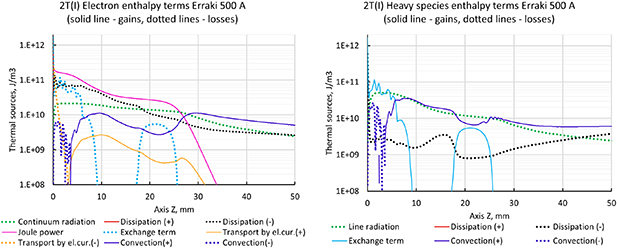
Figure 21. Enthalpy balance in electrons and heavy species along the torch axis (line 1) in the 2T(I) formulation and with radiation loss data from Erraki (1999).
Download figure:
Standard image High-resolution image
Figure 22. Enthalpy balance in electrons and heavy species along the torch axis (line 1) in the 2T(II) formulation and with radiation loss data from Erraki (1999).
Download figure:
Standard image High-resolution imageIn order to draw a parallel between the other studies of 2-T electric arc models and the present study, the 2T(II) formulation can be compared with the transferred arc modeling results from (Freton et al 2012) for the configuration denoted as 'case 5' with the radiation distributed between electrons and heavy species. The following similarities can be found:
- (a)Joule power is the highest electron enthalpy gain near the cathode, but is surpassed by convection in the arc part closer to the anode.
- (b)Convection is a loss near the cathode and gain in the rest of the arc.
- (c)Line radiation is the main loss for the heavy species.
The main difference with the 'case 5' from Freton et al (2012) is that the electron enthalpy dissipation is significantly higher than the other losses in 'case 5'. In this study, the continuum radiation and exchange term are surpassed by the electron enthalpy dissipation only near the cathode, while in the rest these three terms are very close. The assignation of the reactive thermal conductivity to the heavy species explains this difference.
3.2.2. Influence of radiation data.
In the previous section, it has been shown that the ionization energy should be assigned to the electrons which otherwise leads to inconsistent results regarding the exchange term and  . Moreover, the enthalpy balance of heavy species is also dependent on the radiation loss term which may have different data sources as explained above. Consequently, in order to test the influence of the radiation heat loss data on the predictions of the 2-T model, the data from Beulens et al (1991) was embedded to the 2T(II) configuration of the model similarly to Trelles et al (2007), Baeva et al (2016), (2019), Baeva (2017). Figure 23 depicts the electron and heavy species temperatures calculated in the same conditions as figures 14, 19, and 20 (500 A) but using the radiation data from Beulens et al (1991). The thermal disequilibrium degree
  is also shown in figure 23 where the blue areas correspond to
  .
.

Figure 23. Electron and heavy species temperature with 500 A, 2T(II) formulation of enthalpy and radiation data from Beulens et al (1991). Disequilibrium degree θ = Te /Th . The blue area corresponds to θ < 1.
Download figure:
Standard image High-resolution imageIn comparison with figures 14 and 19 where the radiation data from Erraki (1999) are used, significantly higher temperatures are observed in the whole domain due to lower radiation heat loss as seen in figure 24. Moreover,  in a small region at the nozzle exit occurs but with less extension than in figure 20 (2T(I) formulation).

Figure 24. Enthalpy balance in electrons and heavy species along the torch axis (line 1) in the 2T(II) formulation and with radiation loss data from Beulens et al (1991).
Download figure:
Standard image High-resolution imageThe radial profile of the electron temperature at nozzle exit displayed in figure 25 confirms the overestimation of the electron temperature obtained with the Beulens data close to the torch axis. Actually, as shown in figure 9 and also in figure 25, the Beulens radiation data are valid only up to 15,000 K.

Figure 25. Radial electron temperature profiles species at the nozzle exit (line 3) with 500 A, 2T(II) formulation and radiation loss data from Erraki (1999) and Beulens et al (1991).
Download figure:
Standard image High-resolution imageThe enthalpy balances shown in figure 24 highlight lower radiation in the hot region compared to figure 22. The heat dissipation has a much higher role in the enthalpy balance than with the data from Erraki (1999) for both electrons and heavy species due to the higher gradients of both temperatures.
Beyond 30 mm from the cathode tip, where the Joule power decreases to zero, the enthalpy balance of electrons is mainly made between convection and enthalpy dissipation. Meanwhile, the exchange term collapses due to  because of too low line radiation losses of heavy species in the hot region upstream of the anode. In other words, the radiation losses of heavy species are not sufficient to establish a proper enthalpy balance in the model.
Attention is hereafter paid to the influence of the arc current on the disequilibrium degree keeping the same other calculation conditions as in figure 23. Figure 26 shows the electron and heavy species temperatures calculated with I = 100 A. As expected, the maximum temperature is significantly lower than with I = 500 A and remains below 15,000 K. Therefore, the radiation heat loss from Beulens et al (1991) in the obtained temperature range is close to the data from Erraki (1999) and the thermal disequilibrium degree is never below unity at such a low arc current.

Figure 26. Electron and heavy species temperature with 100 A, 2T(II) formulation of enthalpy and radiation data from Beulens et al (1991). Disequilibrium degree θ = Te /Th .
Download figure:
Standard image High-resolution imageAs seen in figure 26, some axial asymmetry of the electron and heavy species temperature is observed near the anode. Such asymmetry was not found in the simulations with 500 A with both formulations of enthalpy and both sources of radiation loss data (figures 14, 19 and 23). The asymmetry seems to be conditioned by the low electron temperature in the vicinity of the anode surface and hence too low electrical conductivity, which causes fluctuations of the anode arc attachment. In order to illustrate these fluctuations, the electric current density over several cross-sections perpendicular to the torch axis is shown in figure 27. It is seen that the electric current density is axisymmetric upstream of the anode, while at the anode some deviation from axial symmetry is found. The electric current is still spread over the whole circumference of the anode, but it is much less uniform than with 500 A. It is worth noting that, in reality, the SinplexPro plasma torch operated at the low current of 100 A is in fact not stable. The measured voltage does not oscillate but drifts almost randomly with the current of 100 A.
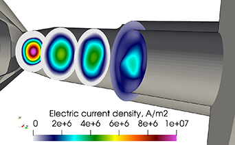
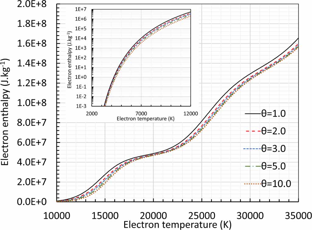
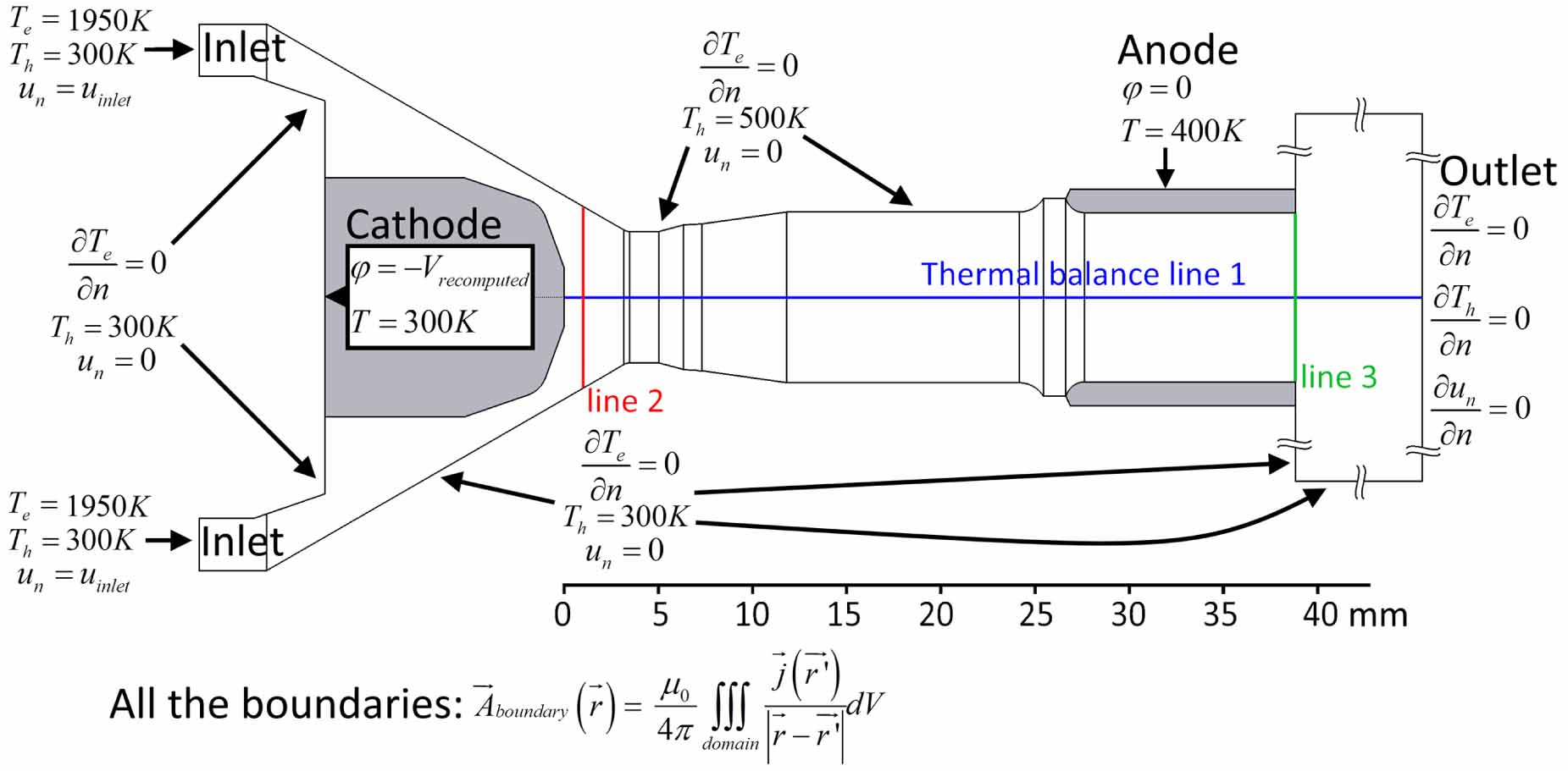
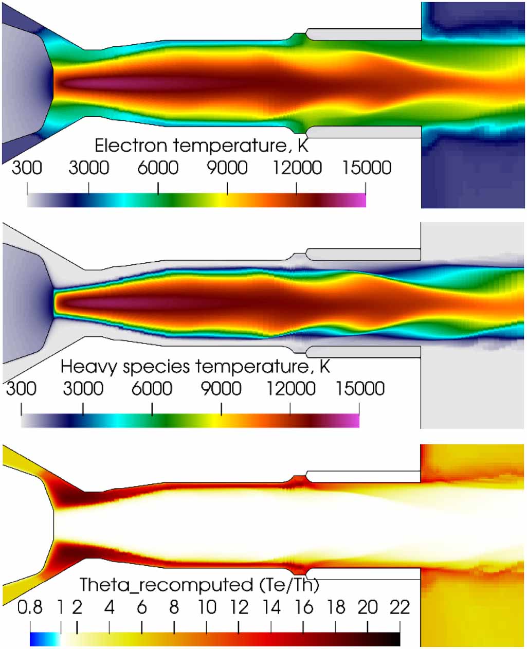
Figure 27. Electric current density over several cross-sections perpendicular to the torch axis with 100 A, 2T(II) formulation of enthalpy and radiation data from Beulens et al (1991).
Download figure:
Standard image High-resolution image
4. Conclusion
Two enthalpy formulations of a two-temperature arc model were tested in the context of cascaded-anode plasma torch. The 2T(I) formulation assigns the ionization part of enthalpy to the heavy species, while the 2T(II) formulation assigns it to the electrons.
The 2T(I) formulation assumes a low storage of enthalpy in electrons and high storage in the heavy species. The 2T(I) formulation makes the contribution of the enthalpy losses too high to the enthalpy balance of electrons, resulting in the unphysical prediction of the electron temperature lower than the heavy species temperature or  in a large area inside the torch and in the whole plasma flow outside the torch. Electrons heat up at the cathode and cool down on the way towards the outside domain faster with the 2T(I) formulation. This means a lower thermal inertia of electrons with the 2T(I) formulation. This formulation brings about an unclear situation of the computation of the plasma properties for
  especially when the radiation heat loss is significant.
In addition, the 2T(I) enthalpy balance leads to the fluctuations of heavy species temperature,  and consequently the exchange term. Such instabilities impose a smaller time step of 10−8 s and higher computational cost of the 2T(I) formulation. The combination of all the disadvantages of the 2T(I) formulation, especially
  in a large area, makes this formulation unsuitable for plasma torch simulation.
The higher storage of enthalpy in the heavy species with the 2T(I) formulation results in higher values of the heavy species enthalpy gain and loss due to convection. On the contrary, since the storage of enthalpy in electrons is higher with the 2T(II) formulation, the electron enthalpy gain and loss due to convection have higher values with this formulation.
The 2T(II) formulation of enthalpy provides more physically valid results, meaning that the heavy species temperature does not get higher than the electron temperature. This is why the 2T(II) formulation is considered more suitable for the simulation of the electric arc in a plasma torch.
The enthalpy balance with the 2T(II) formulation is more stable and without noticeable fluctuations in the exchange term, which allows to use the time step of 10−7 s. This is another advantage of the 2T(II) formulation which makes its computation cost lower.
However, the radiation heat loss data must be properly selected with respect to the simulated operational parameters of the plasma torch. The theoretically correct formulation with proper distribution of radiation heat losses between electrons and heavy species described in Freton et al (2012) can still result in unphysical situation with  if the selected radiation heat loss data are not accurate in the operating temperature range.
Further development of the model includes the consideration of gas mixtures like Ar/H2 or Ar/He that will affect the arc properties and probably the arc attachment mode at anode wall as well. Such gas mixtures will better address the needs of the industry. At last, the inclusion of a cathode sheath model will improve the prediction of the cathode arc attachment.
Acknowledgments
We thank Oerlikon Metco and the region Nouvelle-Aquitaine (France) for funding this study and Yvan Fournier from Électricité de France R&D for his help in development of the 2-T model.
Data availability statement
All data that support the findings of this study are included within the article (and any supplementary files).