

Abstract
The Aral Sea desiccation is one of the worst aquatic ecological disasters of the last century, important for understanding the worldwide trends to degradation of arid lakes under water use and climate change. Formerly the fourth largest lake worldwide, the Aral Sea has lost ∼90% of its water since the early 1960s due to irrigation in its drainage basin. Our survey on the seasonal thermal and mixing regime in Chernyshev—a semi-isolated hypersaline part of the Aral Sea—revealed a newly formed two-layered structure with strong gradients of salinity and water transparency at mid-depths. As a result, the Chernyshev effectively accumulates solar energy, creating a temperature maximum at the water depth of ∼5 m with temperatures up to 37 °C. Herewith, this part of the Aral Sea has evolved to an unprecedently large (∼80 km2) heliothermal lake akin to artificial solar ponds used for 'green energy' production. The newly formed heliothermal lake, with transparent and freshened layer on top of the hypersaline and nutrient-rich deep water, acts as a solar energy trap and facilitates intense biogeochemical processes. The latter reveal themselves in practically 100% opacity of the deep layer to the solar light, permanent deep anoxia, and growing methane concentrations. The recent emergence of the Chernyshev as a heliothermal lake provides an opportunity for tracing the biogeochemical and ecological response of aquatic ecosystems to suddenly changed environmental conditions.
Export citation and abstract BibTeX RIS

Original content from this work may be used under the terms of the Creative Commons Attribution 4.0 license. Any further distribution of this work must maintain attribution to the author(s) and the title of the work, journal citation and DOI.
1. Introduction
Lakes and reservoirs of arid zones are especially sensitive to both climate change and anthropogenic alterations of the regional hydrological cycle [1–3]. Human use of freshwater resources, including irrigation, is particularly extensive in the arid regions that imposes additional stress on the catchment areas resulting in desiccation and shrinking of lakes [4, 5]. Many large lakes worldwide, e.g. Lake Chad, Lake Urmia, the Dead Sea2, suffer from severe lack of water inflow. These arid terminal lakes are prone to salinization, which suppresses vertical mixing by stratification build-up. The mixing regime of saline lakes can be meromictic (supplementary table S1 (available online at stacks.iop.org/ERL/16/115009/mmedia)) [6, 7], with salt stratification preventing exchange of waters between different layers. Existing climate scenarios [8, 9] reveal alarming worldwide trends towards the increase of lake stratification especially in the arid regions.
The infamous case of the Aral Sea, terminal arid lake situated at the border between Kazakhstan and Uzbekistan, demonstrates how anthropogenic and climatic alteration of the regional water budget may change the mixing regime of lakes. Since 1961 diversions of freshwater inflow led to a rapid decrease of the lake's volume [10, 11]. After losing about 90% of its surface area, the formerly brackish dimictic lake turned into several (semi-)separated water bodies with significantly diverging hydrological and biogeochemical conditions [12]. The largest residual basin—the Large (Southern) Aral—revealed increase of the water mineralization from ∼11 g kg−1 up to >200 g kg−1, accompanied by formation of the vertical haline stratification in the water column and a temperature inversion in the bottom layer [10, 13–15]. Strong haline stratification with anoxic conditions in the near-bottom layer was earlier observed in the northern part of the Large Aral, the former Chernyshev Bay [16], accompanied by a complex layered vertical temperature pattern in October 2014 [12]: an intermediate temperature maximum with values of 24.4 ℃ at 6.3 m depth underlaid the 11.2 ℃-warm upper mixed layer, thus exhibiting vertical temperature gradients of ∼10 ℃ m−1. The bottom temperature values reached 15.0 ℃ that was 4.2 ℃ higher than that at the surface. The strong vertical stratification and the warm bottom layer suggested meromictic regime of the basin, requiring however additional observations and analysis to be validated and quantified. For this purpose, we traced the seasonal thermal and biogeochemical regimes of Chernyshev by using autonomous temperature and oxygen measurements, vertical profiling of water quality parameters, and heat budget modeling. This first evaluation of the seasonal regime in the Aral Sea since 1980s reveals a strong vertical stratification, which facilitates heat accumulation below the mixed layer and affects various biogeochemical processes, such as oxygen consumption, production of methane, and nutrients cycling. The more than tenfold increase of salinity within several decades followed by formation of meromixis and strong (>20 K m−1) vertical temperature gradients is unprecedently rapid for large natural lakes. As a result, the newly established thermal regime turned Chernyshev to the largest known heliothermal lake.
2. Data and methods
2.1. Field observations
Two short-term intense field surveys were carried out in Chernyshev on 13–17 October 2015 and 24–28 June 2016 including in situ measurements and water sampling at stations forming a cross-section across the deepest part of Chernyshev (figure 1). The in situ measurements at each station included vertical profiling of major physical–chemical characteristics and water sampling. Profiles of conductivity, temperature, depth, fluorescence and turbidity were taken in October 2015 with a SBE19plus profiler (SeaBird Scientific, USA), and in June 2016 with a Rinko CTD-Profiler (JFE Advantech, Japan), measuring the same characteristics plus dissolved oxygen (DO) content. Measurements of conductivity and fluorescence had been later discarded since the sensors malfunctioned in the hypersaline waters. Additionally, water transparency was measured using the standard Secchi disk. Water samples were taken by a 5 l Niskin Hydro-Bios bottle and analyzed later in laboratory for salinity by the gravimetric method [17].
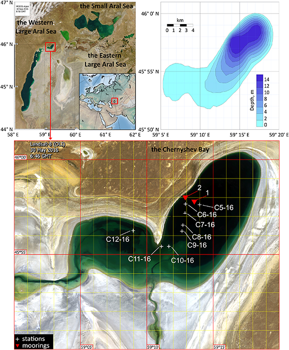
Figure 1. MODIS satellite image of the Aral Sea study area, Landsat-8 satellite image of the Chernyshev Bay of the Large Aral Sea with scheme of the stations and moorings locations and approximate bathymetry of the Chernyshev Bay.
Download figure:
Standard image High-resolution imageContinuous measurements of temperature and DO were conducted at two mooring stations (figure 1). Station 1 was installed at 14 m total water depth and was equipped with 12 temperature loggers TD-1060 (RBR Ltd, Canada) at depths of 2, 3, 4, 5, 6, 7, 8, 9, 10, 11, 12, and 14 m. Six DO loggers D-Opto (Zebra Tech, New Zealand) were added at 2, 4, 8, 10, and 13 m depths. Station 2 was set at 10 m water depth and was equipped with ten TD-1060 loggers at water depths of 1, 2, 3, 4, 5, 6, 7, 8, 9, 10 m. The sampling period was set to 20 s for temperature and 1 h for DO measurements. Stations were deployed on 13 October 2015 and recovered on 26 June 2016. Depth-resolved measurements were however available for the period from 13 October to 21 November 2015 only. Later, when the surface water temperatures approached ∼0 °C, the dissolved salts started to crystallize on the upper part of the moorings and caused their eventual sinking to the bottom (supplementary figure S3). Afterwards, temperature and DO measurements were available only from the bottom, showing a constant temperature of 15.2 °C and zero oxygen content over the winter.
2.2. Heat transport across the water column
Damping of the vertical heat transport across the water column is the critical process leading to the meromixis formation. The time-depth temperature data collected between 13 October 2015 and 21 November 2015 allow direct estimation of the vertical mixing rates. To calculate the net vertical heat flux QTOTAL (z) across the lake water column and the vertical turbulent diffusion coefficient KZ we applied the inverse solution of the heat transport equation,
where T (t, z) is the temperature [K] at time t [s] and depth z [m], Qtotal (t, z) = Qturb (t, z) + QI (t, z) + Qc (t, z) is the bulk kinematic vertical heat flux [K m s−1], whose three major components are the turbulent exchange Qturb (z, t), the short-wave solar radiation QI (t, z), and the conductive (molecular) flux Qc (t, z). Integration of equation (1) from the bottom z = H to some depth z yields the expression for the vertical profile of the heat flux
where the water-sediment heat flux Qtotal (H) can be assumed negligible, since ∂T/∂t|H ≈ 0 и ∂T/∂z|H ≈ 0 from the observations. Assuming further that no solar radiation QI (t, z) penetrates below the layer of strong turbidity and salinity gradients z = hSML (figure 2(a) and supplementary video 1), where hSML is the depth of the surface mixed layer, Qtotal (t, z) ≈ Qturb (t, z) + Qc (t, z) = [Kz (z) + κ] ∂T (t, z)∂z−1, and one can calculate the vertical diffusion coefficient KZ from
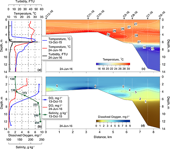
Figure 2. Chemical and thermal stratification in Chernyshev. Vertical profiles of (a) temperature and turbidity (Formazin Turbidity Unit (FTU)) and (b) salinity and DO concentration taken in the central part of Chernyshev (Station C5-16, figure 1) on 13 October 2015 and on 24 June 2016. Transects of (c) temperature and (d) DO concentration on 24 June 2016.
Download figure:
Standard image High-resolution imagewhere κ = Qc (∂T/∂z)−1 = O (10−7) m2s−1 is the molecular heat conduction coefficient. The net flux at the lake surface Qs was estimated from extrapolation of the flux profile in the surface mixed layer (SML). For a mixed layer with homogeneous vertical temperature distribution (0 ⩽ z ⩽ hSML), a linear vertical flux distribution follows directly from equation (1) and is supported by our calculations (figure 3(b)):
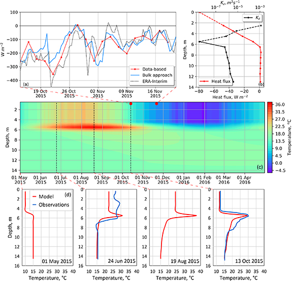
Figure 3. (a) Net surface heat flux (sum of sensible and latent heat fluxes and long wave radiation balance, positive downward) according to observations, bulk formulae calculations and ERA-Interim reanalysis (13 October–21 November 2015). (b) Profiles of vertical heat flux (red line) and vertical heat exchange coefficient (black line) within the water column averaged over the entire period of observations, dashed red line implies extrapolation to the surface, dashed black line implies approximate estimations. (c) Model reconstruction of the seasonal thermal cycle. (d) Vertical temperature profiles from the model in comparison with available CTD-measurements carried out in June 2016 and October 2015.
Download figure:
Standard image High-resolution imageHerewith, the surface flux Qs can be calculated by linear extrapolation of equation (2) to the water surface as Qs = Qtotal (z1) − (Qtotal (z2) − Qtotal (z1)) z1/(z2 − z1), where z1 and z2 > z1 are any two depths within the SML, at which Qtotal is calculated from equation (2). We used the two uppermost calculation depths z1 = 2.5 and z2 = 3.5 m for the data from the mooring Station 1.
Short-term diurnal and sub-diurnal temperature variations have correspondingly smaller spatial scales, for which the 1 m vertical resolution of measurements can appear too coarse, resulting in unrealistic flux fluctuations. To filter out diurnal variations from the seasonal heat budget, the original time series of temperature were averaged over 48 h prior the calculations. As an independent cross-validation, the estimates of the surface heat flux were compared with the sum of sensible and latent heat fluxes from ERA-Interim reanalysis [18] and with the surface fluxes computed by the bulk aerodynamic approach [19] using the measured surface water temperatures as input. Thereby, the backward lake effect on the air–land interaction was indirectly estimated by comparison of the ERA-based results (no lake effect) vs measurement-based fluxes.
2.3. Model of the annual temperature cycle
To estimate the seasonal variability in the heat budget, we applied a one-dimensional (1D) two-layered heat budget and temperature model. The model is aimed at (a) revealing the major physical mechanisms producing the heliothermal behavior of the lake, (b) reconstruction the seasonal variability in the heat budget, (c) estimation of the subsurface temperature maximum lifetime and the range of the temperature variations within it, and (d) estimation of the heat accumulation rate in the deep monimolimnion. The model is based on the heat conservation only, without any artificial fitting to the observed temperatures and is validated by comparison of the modeling results against the observed temperatures. Thereby, the model provided the opportunity to quantify the seasonal balance of the heat sources and sinks, which leads to the formation of the heliothermal regime. Based on the empirical evidence, the model assumptions were formulated as follows:
- The vertical position of the chemocline remains constant.
- The vertical turbulent flux across the chemocline is negligible.
- The temperature profile in the SML (mixolimnion) is homogeneous.
- No solar radiation penetrates beneath the chemocline.
Using KZ from equation (3) as a seasonal-mean estimation, the accumulation of heat in the deep monimolimnion (hSML < z < H) is estimated as
with the boundary conditions at the bottom, z = H,
At the top of the monimolimnion, the temperature jump produced by absorption of solar radiation is balanced by the nearly conductive heat flux,

where γ is the extinction coefficient in the one-band exponential radiation decay, KZ (hSML) ≈ κ= 10−7 m2s−1. In the SML, temperature is modeled by integration of equation (1) from the surface to z = hSML
where Qb is the heat flux at the SML base.
The surface heat flux Qs is calculated from the air-lake heat balance [19] using the surface water temperatures at the previous time step and atmospheric characteristics from the ERA-Interim reanalysis. The chemocline is simulated in the model by a zero-thickness layer at z = hSML, with the heat flux across it Qb = χ(T (0) − TSML). The heat transfer rate across the chemocline is parameterized as χ = 2.7 × 10⁻⁷ m s−1 that corresponds to molecular heat flux across a 0.5 m thick layer. As initial condition, T (z) = const = T (H) = 15 °C (corresponding to the measured annually constant temperature of the deep monimolimnion) and TSML= 10 °C (roughly corresponding to the 'equilibrium' water surface temperature approximated as the annual mean air temperature) were used, corresponding to some date t0 at the initial stage of the summer heating period, when the mixolimnion stayed colder than monimolimnion and stability of the water column was controlled by salinity gradient. After several test model runs, t0 was set to 1 May 2015, whereas the model was weakly sensitive to the variation of the date within ∼30 days interval. The radiation extinction coefficient γ was set to 0.4 m−1, based on Secchi disc measurements and model sensitivity experiments. Equations (5)–(8) were solved numerically using a Python script.
3. Results
3.1. Vertical structure of the water column
The area and the mean depth of Chernyshev at the moment of measurements varied around ∼80 km2 and 4 m, respectively, with the maximum depth of about 15 m (figure 1). Chernyshev remains connected to the Large Aral through a narrow straight in its south, and, intermittently, to ephemeral lakes on the dry bottom of the former Aral Sea in the east (figure 1). The current water budget is unknown, consisting presumably from episodic releases of water from the Small Aral, meltwater, precipitation-evaporation, and, possibly, groundwater discharge.
Salinity of the lake exhibited a three-layered structure (figure 2(b)): upper mixed layer, a layer with a salinity jump of ∼100 g kg−1 between 4 and 6 m water depth, and a deep nearly homogeneous layer extending to the bottom (in terms of meromixis: mixolimnion, chemocline, and monimolimnion, respectively). In the monimolimnion, salinity slightly increased downwards from 233 to 244 g kg−1 between 6 and 12 m depth. Light conditions varied strongly across the water column: the upper transparent layer had sharp lower boundary with turbidity peak at the chemocline (figure 2(a)). Underneath, turbidity decreased, but remained twice as high as those in the mixolimnion. A vivid qualitative picture of the transparency changes in the chemocline is provided by the underwater camera moving from water surface down to the bottom (supplementary video 1): the water column beneath the chemocline remains completely impermeable to the solar radiation beneath the sharp turbidity peak. The white (Secchi) disc measured transparency depth of 6.5 m, which value corresponded to the depth of the turbidity peak and likely underestimated the transparency of the upper layer.
Vertical profiling in the middle of the autumn cooling period (October 2015) and in the middle of the summer heating period (June 2016) provided an estimation of the range of seasonal temperature and oxygen variations (figure 2(a)): the most striking feature of the thermal regime is the formation of the mid-depth temperature inversion in October with the downward temperature increase from 12.5 ℃ at the water surface to the maximum of 30.7 ℃ at ∼5 m depth. This subsurface temperature maximum was followed by a gradual temperature decrease down to 8–9 m depth and a homogenous deep layer with temperature values about 15.2 ℃ extending to the bottom. According to the ERA Interim reanalysis data [18], the mean air temperatures for the period 10–15 October 2015 amounted at 0.0 ℃ with the minimum of −5.7 ℃. The inversion degraded in summer (figure 2(a)), when the upper mixolimnion was heated up to 29.4 ℃.
The mixolimnion was well-oxygenized, with DO concentrations close to 70%–80% of saturation (9.0 mg l−1 in October and 5.5 mg l−1 in June, note that the real absolute concentrations may differ due to effects of the high salinity on DO solubility). Under the chemocline, the environment was completely anoxic throughout the year (figure 2(b)).
The spatial structure of temperature and DO followed the three-layered meromictic pattern (figures 2(a) and (b)): the vertically homogeneous mixolimnion was well-saturated with oxygen and revealed strong seasonal temperature variations. In turn, beneath the ∼6.5 m depth, the oxygen was absent, and temperatures remained at the nearly constant value of 15.2 ℃ beneath ∼10 m depth. Radial transects demonstrated the persistence of the three-layered structure across the lake (figures 2(c) and (d)).
3.2. Temporal evolution of temperature and vertical heat transport
Reliable continuous temperature and DO records from autonomous moored stations were available from 13 October to 21 November 2015 only. Later, the submerged temperature-oxygen chains started to gradually sink due to crystallization of salt on buoys and sensors in cold surface waters and eventually drowned to the bottom around 31 December (see section 2 and supplementary information 1). Nevertheless, the mooring data provide a valuable insight into the heat storage and vertical heat transport: during the intense cooling of the mixolimnion, temperatures in the upper mixed layer decreased from 12.5 ℃ on 13 October to 2.6 ℃ on 21 November, while the intermediate temperature maximum decreased from 30.6 °C to 21.8 °C (figures S2(a) and (b)). Herewith, the temperatures in the chemocline in November remained ∼6.2 ℃ higher than at the bottom, ∼19.2 ℃ higher than at the surface, and >27 ℃ higher than the minimum air temperatures. The vertical position of the chemocline was constant, so that the autumn cooling affected only the upper water column, without entrainment of cold surface water into the monimolimnion. Correspondingly, anoxic conditions in the bottom layer along with the temperature values of 15.2 ℃ remained stable beneath the chemocline. Salt precipitation started after the mixolimnion temperatures dropped to ∼3 °C (supplementary figures S1–S3) causing gradual sinking of the moorings. The lowest temperatures in the mixolimnion of ∼0 °C were measured around 20–25 December; afterwards, all sensors settled on the bottom and continued to record during January–June 2016 constant temperatures of 15.2 °C and zero DO content (supplementary figure S1).
The surface heat fluxes (figure 3(a)) demonstrated a strong (100–200 W m−2) heat release to the atmosphere from the upper mixolimnion, contributed mostly by evaporation. The ERA-interim reanalysis showcased a higher amplitude of the flux variability than data-based calculations, indicating the damping effect of the lake on the air-land heat exchange not accounted for in the reanalysis calculations. The vertical profiles of the heat flux Qtotal (z) and the vertical exchange coefficient Kz (z) averaged over the period of moored observations (figure 3(b)) showed strong mixing in the mixolimnion with linear decrease of Qtotal (z) from the maximum at the water surface to nearly zero in the chemocline, characteristic of the well-mixed surface layer with homogeneous vertical temperature distribution (equation (1)). Kz in the chemocline dropped to the level of the purely conductive exchange, close to the molecular heat conductivity κ ≈ 107 m2s−1, showcasing effective cancellation of the vertical transport by the density (salinity) gradient in the chemocline. Herewith, the strong surface cooling (figure 3(a)) and cancelling of the heat flux in the chemocline at ∼6 m depth (figure 3(b)) can be identified as the ultimate mechanisms resulting in the intermediate temperature maximum formation (figure 3(c)). In the deeper monimolimnion, Kz varied around the value 10κ, characteristic of non-zero vertical turbulent mixing rates, though orders of magnitude smaller than in the surface layer. The mixing in the wind-isolated monimolimnion is apparently enhanced by internal waves, which have been shown to produce the same tenfold increase of the background mixing over the molecular level in stratified lakes isolated from the atmosphere by the ice cover [20, 21].
3.3. Reconstruction of the seasonal thermal cycle
The model simulated maximum subsurface temperatures of up to 37.4 °C in mid-August (figure 3(c)) caused by accumulation of solar radiation in the chemocline. Maximum inverse temperature gradients at the base of the upper mixed layer reach 18.2 K m−1 in late October, in a good agreement with temperature measurements (figure 3(d)). The summer temperatures also agreed qualitatively with the observations, with larger deviations in the upper mixed layer, where the model assumes vertical homogeneity, but the real temperature profiles are affected by short-term diurnal fluctuations. The heat storage in the deep monimolimnion (8–12 m depth from the surface) stays nearly constant; the bottom temperature increases at ∼0.8 °C per annum. The latter value implies continuous accumulation of heat by Chernyshev on inter-annual time scales, but should be treated with care, because 1D models are prone to underestimate the near-bottom mixing [22, 23].
4. Discussion and conclusions
Our data unambiguously show that the former bay of the Aral Sea—Chernyshev—turned to a meromictic heliothermal water body [24] with extreme temperature, light and chemical regimes: complete isolation of the deep waters from the solar light, the strong salinity jump and the intermediate temperature maximum at the top of the deep layer; constraint of the seasonal temperature variations by the upper layer; isothermal and oxygen-free conditions near the lake bottom in the annual cycle.
Among less than 30 heliothermal waters worldwide known so far [25], Chernyshev with its area of ∼80–90 km2 is the largest heliothermal lake, the second one being permanently ice-covered Antarctic Lake Vanda [26] with the area of 5.2 km2 and temperatures in non-convective bottom layer of 25 °C. Moreover, Chernyshev is also the youngest heliothermal lake, emerged within the last half-century. The two-layered vertical pattern was probably formed by confluence of water masses with different physical properties: extremely saline inflow from the former Eastern Large Aral before its desiccation in the bottom layers [10, 13], and less saline waters from the Western Large Aral in the upper layers. Another plausible scenario of the heliothermal lake formation in place of the former Aral Sea bay refers to the later measures aimed at the Aral Sea basin and the recent positive trends in the regional runoff and precipitation. In mid-2000s, the newly built 'Kok-Aral' dam separated the northern Small Aral from the rest of the former Aral Sea basin [27]. While resulting in an improvement of the ecological state of the Small Aral, the measure was counteracted by the simultaneous increase of precipitation and runoff in the region [5, 28, 29]. As a result, the discharge through the floodgates of the dam remained appreciable during the last decades, manifested by the flooding of the dry bottom southwards from the Small Aral by relatively fresh waters of the Syrdarya River. The waters can reach the Chernyshev area and create a diluted layer on top of it, with a sharp salinity gradient (chemocline) effectively preventing vertical mixing (figure 4). The lower hypersaline and nutrients-reach layer favors high microbial production reducing water transparency, while the upper layer remains oligotrophic and clear-water due to prevention of the upward nutrients transport by the chemocline. The resulting vertical gradient in the water transparency turns the chemocline to a 'solar radiation trap'. Largely similar conditions are observed in estuarine lakes and lead to the formation of an 'mid-depth temperature maximum' [30], but with less sharp gradients. Vertical stratification built-up and the onset of the meromixis in saline lake due to increase of the relatively fresh inflow was also observed in other regulated basins [31]. Noteworthy, this 'exogenous' scenario of meromixis and heliothermality formation might be enforced by endogenous lake-internal dynamics: the upper layer is densely populated by brine shrimp Artemia parthenogenetica [32, 33] (see supplementary video 1), and the dead biological material accumulates at the density gradient in the chemocline, where microbial degradation additionally contributes to the strong peak of turbidity. Formation of thin layers of high microbial activity is common for the strong non-turbulent chemoclines of meromictic lakes [34, 35]. Also, crystallization and precipitation of salts from the surface waters in winter, driven by the strong seasonal variability of the surface temperature might additionally increase the vertical salinity and density gradients.

Figure 4. Possible pathways of heliothermal regime formation in Chernyshev illustrated by a MODIS satellite picture from 23 March 2015, when surface runoff from Small Aral is around its maximum. Green lines mark the path of presumably hyposaline (brackish) water, brown lines mark potentially hypersaline waters.
Download figure:
Standard image High-resolution image
The heliothermal regime of Chernyshev keeps the deep monimolimnion warm (about 15 °C–16 °C) throughout cold winter, turning it to a permanent biogeochemical reactor, with microbial degradation continuing at high rates: total methane content in the basin increased from about 3 × 10⁵ kg in 2015 to about 5 × 10⁵ kg in 2016 [36]. Observed dissolved methane concentrations in the monimolimnion were an order of magnitude higher than those in the anoxic zone of the Black Sea, the largest aquatic methane reservoir in the world. If the rest of the Large Aral Sea outside Chernyshev also features meromictic and heliothermal regime (which is currently not known), the potential methane accumulation may appear several orders of magnitude higher. The energy capture mechanism in heliothermal lakes is similar to artificially constructed brine solar ponds [37], providing a hypothetical potential of practical use of the stored heat. Research on the extremophilic life in the dark hypersaline monimolimnion of Chernyshev is also potentially important for understanding the possible extraterrestrial life forms [38].
Acknowledgments
Authors thank all the participants of the Aral Sea expeditions taken place in 2015–2016. This work is dedicated to the memory of late Igor V Goncharenko, whose invaluable contribution to field research on the Aral Sea made the study possible. Artyom Spirin created the multimedia content.
The study is part of the joint Russian-German Project 'The Aral Sea and Meromixis' funded by the Russian Foundation for Basic Research (RFBR Project No. 20-55-12007) and German Research Foundation (DFG KI 853-16/1). The field surveys were supported by the Ministry of Science and Education of Russia (Theme No. 0128-2021-0001) and German Federal Ministry of Education and Research (BMBF grants 033W034A and 01LP2006A).
Data availability statement
The data that support the findings of this study are available upon reasonable request from the authors.
Author contributions
All authors participated in field surveys and conducted observations. A I and G K processed the data, performed calculations and wrote the text. G K, P Z and A I revised the text with contributions of all co-authors.
Conflict of interest
Authors declare no competing interest.