

Abstract
The United States 'warming hole' is a region in the southeast/central U.S. where observed long-term surface temperature trends are insignificant or negative. We investigate the roles of anthropogenic forcing and internal variability on these trends by systematically examining observed seasonal temperature trends over all time periods of at least 10 years during 1901–2015. Long-term summer cooling in the north central U.S. beginning in the 1930s reflects the recovery from the anomalously warm 'Dust Bowl' of that decade. In the northeast and southern U.S., significant summertime cooling occurs from the early 1950s to the mid 1970s, which we partially attribute to increasing anthropogenic aerosol emissions (median fraction of the observed temperature trends explained is 0.69 and 0.17, respectively). In winter, the northeast and southern U.S. cool significantly from the early 1950s to the early 1990s, but we do not find evidence for a significant aerosol influence. Instead, long-term phase changes in the North Atlantic Oscillation contribute significantly to this cooling in both regions, while the Pacific Decadal Oscillation also contributes significantly to southern U.S. cooling. Rather than stemming from a single cause, the U.S. warming hole reflects both anthropogenic aerosol forcing and internal climate variability, but the dominant drivers vary by season, region, and time period.
Export citation and abstract BibTeX RIS

Original content from this work may be used under the terms of the Creative Commons Attribution 3.0 licence.
Any further distribution of this work must maintain attribution to the author(s) and the title of the work, journal citation and DOI.
1. Introduction
Global surface temperatures have increased by 0.85 °C over the past century while temperatures in the southeast and central United States have cooled slightly (Hartmann et al 2013). This long-term U.S. cooling, referred to as the 'warming hole', has been investigated in a number of observational and model-based studies (supplemental table 1 available at stacks.iop.org/ERL/12/034008/mmedia). These studies examine different time periods, seasons, and metrics, and therefore yield conflicting results as to whether the warming hole is primarily a response to natural variability or anthropogenic forcing. Here we begin to reconcile these disparate studies by providing a systematic approach to characterizing U.S. temperature trends. We demonstrate that anthropogenic aerosols have a significant impact on the warming hole in summer, particularly during the 1950–1970 period, while negative temperature trends during the winter in the second half of the 20th century contain signals of internal climate variability in the ocean and atmosphere.
Past studies have shown that the warming hole is likely influenced by changes in rainfall, soil moisture, and cloud cover over the southeast and central U.S. (Robinson et al 2002, Pan et al 2004, Portmann et al 2009, Leibensperger et al 2012, Meehl et al 2012, Misra et al 2012, Weaver 2012, Yu et al 2014). These hydrological processes, in turn, may be affected by remote changes in Pacific and Atlantic sea surface temperatures (SSTs), either due to internal variability or anthropogenic forcing (Robinson et al 2002, Kunkel et al 2006, Leibensperger et al 2012, Meehl et al 2012, Weaver 2012), and/or by the regional effects of anthropogenic aerosols (Leibensperger et al 2012, Yu et al 2014) and land use changes (Misra et al 2012) over the U.S. Changes in biogenic aerosol abundances may also contribute to the warming hole in summer (Goldstein et al 2009), but currently available observations and models are insufficient to test this hypothesis.
An important element of this discussion is the lack of a single consistent definition of the warming hole across these various studies. Depending on the time period, season, and temperature index considered, the warming hole is found in the central (Robinson et al 2002, Pan et al 2004, Kunkel et al 2006, Wang et al 2009, Weaver 2012), the north central (Portmann et al 2009, Pan et al 2013), the southeast (Portmann et al 2009, Meehl et al 2012, Misra et al 2012, Hartmann et al 2013), or the eastern (Meehl et al 2012, Donat et al 2013) United States (see supplemental table 1). The region of focus matters because surface temperatures in different regions of the U.S. respond to different physical mechanisms; for example, central U.S. surface temperatures are strongly influenced by changes in local hydroclimate driven by shifts in the Great Plains low-level jet (Pan et al 2004, Leibensperger et al 2012, Weaver 2012) in response to changes in Pacific and Atlantic SSTs (Weaver and Nigam 2007, Weaver 2012), whereas the northeast U.S. is sensitive to changes in the summer storm tracks (Folland et al 2009). Similarly, variability in winter and summer surface temperatures in the U.S. is driven by different mechanisms: we expect North Atlantic Oscillation (NAO) variability to be more pronounced in winter (Hurrell et al 2003), while anthropogenic aerosol forcing is stronger in summer due to greater insolation. Finally, as shown in figures 1 and 2, spatial patterns of observed temperature trends over the U.S. vary significantly over different time periods. Over the long-term period 1901–2005, the western and northern regions of the U.S. have warmed more rapidly than the eastern and southern regions of the U.S. in both seasons, a feature which global climate models typically do not capture (Kunkel et al 2006, Kumar et al 2013). However, as shown in the center and right panels of figures 1 and 2, regions of cooling shift to the central, southern, and eastern U.S. over different time periods. The variability in the spatial distribution of temperature trends in figures 1 and 2 serves to highlight the need for a comprehensive exploration of the warming hole over different regions, seasons and time periods.
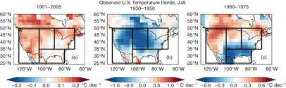
Figure 1 Trends in observed (GISTEMP) surface air temperature (°C/decade) in summer from 1901–2005 (left), 1930–1950 (center), and 1950–1975 (right). The boxes denote the four regions discussed in the paper: the northeast U.S. (35–50°N, 70–90°W), the southern U.S. (25–35°N, 80–105°W), the north central U.S. (35–50°N, 90–105°W), and the western U.S. (25–50°N, 105–125°W).
Download figure:
Standard image High-resolution image
Figure 2 As in figure 1, but for winter.
Download figure:
Standard image High-resolution imageKumar et al (2013) use a moving 30-year window to investigate the dependence of the warming hole on the time period over which temperature trends are computed. We build upon this analysis by systematically examining temperature trends of different lengths for different regions and seasons, assessing the dependence of the trends on the selected start and end years, and identifying physical driving mechanisms. In order to fully characterize the variability in U.S. temperature trends, we analyze winter and summer temperature trends over all possible periods of at least 10 years during 1901–2015 in the four regions shown in figure 1: the northeast U.S. (35–50°N, 70–90°W), the southern U.S. (25–35°N, 80–105°W), the north central U.S. (35–50°N, 90–105°W), and the western U.S. (25–50°N, 105–125°W). These regions are chosen to highlight the areas of maximum cooling in summer in the 1930–1950 and 1950–1975 periods. We show that temperature trends in the U.S. depend on different factors in different seasons and time periods: anthropogenic aerosols play a role in the observed summer warming hole, while the winter warming hole is driven by the Pacific Decadal Oscillation (PDO) and the NAO.
2. Data and methods
We examine observed U.S. monthly mean surface temperature trends from the GISTEMP dataset (GISTEMP Team 2016, Hansen et al 2010), on a 2° × 2° latitude/longitude grid, available from 1880–2015. Linear temperature trends (ten years or longer) are computed using the ordinary least squares method. We assess the statistical significance of trends using a standard t-test, adjusting the sample size to account for autocorrelation as in Santer et al (2000). Additionally, we analyze observed temperature trends using the HadCRUT4 (Morice et al 2012) and NCEP GHCN (Fan and van den Dool 2008) datasets. Our conclusions are robust and independent of the dataset used (supplemental figure 1, supplemental figure 2).
We compare observed surface temperature trends with simulations from 11 global climate models (CanESM2, CCSM4.0, CESM1 CAM5, CSIRO Mk3.6.0, FGOALS-g2, GFDL-CM3, GFDL-ESM2M, GISS-E2-H, GISS-E2-R, IPSL-CM5A-LR, NorESM1-M; see supplemental table 2 for details and references) that represent a subset of models from the Coupled Model Intercomparison Project Phase 5 (CMIP5; Taylor et al 2012). The 11 models were selected because they each performed a full historical simulation (HIST), with all natural and anthropogenic forcings varying from 1850–2005; an 'aerosol only' simulation (AER), with anthropogenic aerosols as the only time-varying forcing and all other forcings held at pre-Industrial levels; and a 'greenhouse gas only' simulation (GHG), with anthropogenic greenhouse gases as the only time-varying forcing. There is large uncertainty in the forcing due to anthropogenic aerosols, but the models considered here cover the range from weak/moderate aerosol forcing (FGOALS-g2, IPSL-CM5A-LR, GISS-E2-R) to strong aerosol forcing (GFDL-CM3, CESM1 CAM5; Boucher et al 2013). We compute the multi-model mean by using the first ensemble member from each of the 11 models so as not to skew the results to favor the forced response from models with larger ensembles. Trends are computed as trends in the multi-model mean.
We additionally examine the effect of SST forcing on U.S. temperature trends using a 16-member ensemble of Global Ocean Global Atmosphere (GOGA) simulations (Guo et al 2016). The GOGA simulations were performed with the National Center for Atmospheric Research Community Atmosphere Model version 5 (NCAR CAM5), with an Eulerian spectral dy-core in T42 horizontal resolution and 30 vertical levels. The NCAR CAM5-GOGA experiment is coupled to the interactive Community Land Model version 4 (CLM4) and the Los Alamos Sea Ice Model version 4 (CICE4) with prescribed sea ice concentrations. The observed Hadley center SST and sea ice (Rayner et al 2003) for the period 1870 to 2014 are prescribed over the global oceans. These simulations are designed to test the atmospheric response to observed changes in SSTs and evaluate the contribution of SSTs to the warming hole.
3. Location and timing of the summer warming hole: a role for aerosols and internal variability
We begin by examining U.S. surface temperature trends during summer. The panels on the left of figure 3 show the observed trends in mean summer temperatures in each U.S. region (see figure 1) as a function of the start (horizontal axis) and end years (vertical axis). In the north central U.S., the sign of the long-term trends (50 or more years) depends on the time period considered. Trends starting in the 1930s are negative (see also figure 1(b)), while those starting before or after the 1930s are generally positive (figure 3(a)). The 1930s were an exceptionally hot and dry decade in the U.S., commonly known as the 'Dust Bowl'. For example, the summers of 1934 and 1936 remain two of the hottest on record, particularly in the north central U.S. (Peterson et al 2013, Donat et al 2016). The Dust Bowl was most likely the result of internal variability in Pacific SSTs (Schubert et al 2004, Seager et al 2008, Donat et al 2016), potentially amplified by dust aerosol and land use changes (Cook et al 2009), and/or by internal atmospheric variability (Hoerling et al 2009). Negative summertime temperature trends in the north central U.S. starting in the 1930s reflect their start date occurring during the Dust Bowl, and can be interpreted as a recovery from this anomalously warm decade. Trends in the northeast are also influenced by a period of high temperatures in the 1930s associated with the Dust Bowl (figure 3(d)). This should be borne in mind when considering studies (Kunkel et al 2006, Leibensperger et al 2012) that analyze temperature trends starting in this time period. Long-term summertime temperature trends in the southern U.S. starting prior to 1955 are generally not significant (figure 3(g)). Temperatures decrease from the 1950s to the mid 1970s in all three regions, most strongly in the southern U.S. Long-term temperature trends ending in the 2000s in the western U.S. are uniformly positive (figure 3(j)).

Figure 3 Trends in summertime mean surface temperatures (°C /decade) from GISTEMP (left) and the multi-model mean historical forcing scenario from CMIP5 (middle) in the north central U.S. (a), (b), northeast U.S. (d), (e), southern U.S. (g), (h), and western U.S. (j), (k). The colours show the value of the trend as a function of the start and end years of the time period considered. Trends that are not significantly different from zero at the 95% confidence level are whited out. The right panels show the regional time series of summertime mean temperature anomalies from GISTEMP (black), the historical all forcing scenario (red), the aerosol only scenario (blue), and the greenhouse gas only scenario (green). Orange shading shows the range of the individual models in the historical scenario. All temperatures are anomalies with respect to 1901–2005 averages.
Download figure:
Standard image High-resolution imageThe CMIP5 HIST multi-model mean captures the timing of transitions between positive and negative trends in observed summertime temperatures in the northeast and southern U.S. over the latter half of the 20th century (compare figures 3(e) and (h) with figures 3(d) and (g)). Outside of the north central U.S., where the observed summer temperature trends are strongly influenced by the 1930s Dust Bowl, the multi-model mean temperature time series is significantly correlated with the observed temperature (table 1). This correlation suggests a role for external forcing in driving temperature trends in the U.S., as by averaging over the CMIP5 ensemble, we are increasing the signal (anthropogenic climate change) to noise (internal variability) ratio. We note, however, that the magnitude of the modeled trends is generally less than observed, implying that internal variability (reduced by averaging) also contributed to the observed trends, and/or that the forced response is too weak in the CMIP5 models. The multi-model mean, which tends to average out internal variability, does not produce a Dust Bowl, and therefore does not reproduce the observed cooling in the north central U.S. beginning in the 1930s. CMIP5 models capture the positive hundred-year temperature trends in the western U.S., implying a forced response to rising greenhouse gases (figures 3(k) and (l)). Outside of the north central U.S., temperature trends from 1970 onwards are significantly positive in both the observations and the CMIP5 multi-model mean. This is most likely due to increased positive forcing from greenhouse gases combined with reductions in the negative forcing due to aerosols (figure 3, supplemental figure 3).
Table 1. Correlation coefficients (r) between the observed and CMIP5 multi-model mean regional surface temperature time series from 1901–2005. Bolded values are significant at the 95% confidence level. The significance of correlations is evaluated with a t-test.
| Summer (JJA) | Winter (DJF) | |
|---|---|---|
| North Central U.S. | 0.10 | 0.13 |
| Northeast U.S. | 0.26 | 0.13 |
| South U.S. | 0.29 | −0.12 |
| Western U.S. | 0.40 | 0.13 |
As the second half of the twentieth century has been a focus in the warming hole literature, we examine this period more closely. Several studies have attributed the U.S. warming hole to forcing by U.S. anthropogenic aerosols (Leibensperger et al 2012, Yu et al 2014). Figure 3 shows significant observed cooling from the 1950s to the mid-1970s in the southern and northeast U.S. and to a lesser extent in the north central U.S. (see also figure 1(c)). These trends are qualitatively captured by the CMIP5 models. In the northeast U.S., the HIST scenario captures most of the magnitude of the observed trends from the 1950s (start dates between 1950 and 1954) to the mid 1970s (end dates between 1973 and 1976), with a median ratio of modeled to observed trends of 0.69. In the southern U.S., HIST captures the timing of the negative trends, but does not produce the full magnitude of the observed trends with a median ratio of 0.17. The HIST, AER, and GHG scenarios in figures 3(c), (f) and (i), and supplemental figure 3 indicate that the mid-century cooling trends in the CMIP5 models are at least in part a forced response to rising anthropogenic aerosols.
Although the CMIP5 multi-model mean qualitatively captures the observed cooling in the southern and northeast U.S. during 1950–1975, it does not reproduce the observed spatial pattern of temperature trends during this period (figure 4(c) vs. figure 1(c)). However, the observations represent a single realization of the climate system, while the multi-model mean is a composite of 11 models that averages over internal variability with the goal of identifying the forced response. When we compare the observations to individual ensemble members from each model, we can find in many of the models at least one ensemble member that captures features of the observed warming hole, with cooling in the eastern and/or southern U.S. (supplemental figure 4). We also find in many of the models at least one ensemble member that produces a pattern that is spatially anti-correlated with the observations, with warming in the eastern and/or southern U.S. (supplemental figure 5). We conclude that cooling in the U.S. during this period is influenced by anthropogenic aerosols, but that the specific spatial pattern of observed temperature change, with cooling in the south central and eastern U.S. and warming in the western U.S., is likely to be strongly influenced by internal variability.

Figure 4 As in figure 1, but for the CMIP5 multi-model mean (HIST).
Download figure:
Standard image High-resolution image4. Winter cooling trends linked to the PDO and NAO
Interannual variability of surface temperature is significantly enhanced in winter as compared with summer (figure 5), confounding detection of significant temperature trends on decadal-to-multidecadal time scales. Observed long-term wintertime temperature trends in the north central U.S. depend somewhat on the start and end year, but are generally positive (figure 5(a)). In the northeast and southern U.S., long-term trends beginning prior to 1950 are generally small or negative, while significant warming occurs between 1950 and the present. As was the case in summer, the observed long-term wintertime temperature trends in the western U.S. are generally positive. Notably, there is significant mid-century cooling over most of the U.S., most pronounced in the southern U.S., which we examine further below.

Figure 5 As in figure 3, but for winter.
Download figure:
Standard image High-resolution imageThe left and middle columns of figure 5, as well as the correlation values in table 1, indicate that the CMIP5 multi-model mean does not capture the observed mid-century negative temperature trends in the northeast and southern U.S., suggesting that these trends may be the result of internal variability rather than a forced response. In agreement with the results of Meehl et al (2012) and Weaver (2012), we find that observed winter temperatures in the southern U.S. are significantly anti-correlated with the PDO index from 1901 to 2010 (r = −0.37, figure 6). Given this relationship, we can estimate the contribution of the PDO to regional temperature trends by first regressing the regionally averaged temperature T against the PDO index such that:

where α and β are estimated using detrended temperature and PDO time series and ε represents the residuals. The component of the regional temperature trend that is linearly congruent with the PDO is then given by:
where dPDO/dt is the trend in the PDO index. Using this approach, we estimate that multidecadal changes in the PDO, which are marked by a shift from negative to positive around 1976/77, contribute to as much as half of the observed negative temperature trend from 1950–1990 in the southern U.S. (figure 6(a)). The shift of the PDO from positive to negative also accounts for 25%–50% of the observed positive temperature trends in this region from the 1980s to present (figure 6; Meehl et al 2015).

Figure 6 Comparisons between observed wintertime surface temperature in the southern U.S. and the PDO index (Zhang et al 1997). (a) The ratio of the temperature trends in the regressed PDO index (see text) to the observed trends. Time periods where the observed trend is insignificant are whited out. (b) The time series of the observed temperature anomalies (black) and the PDO Index (blue). All time series are anomalies with respect to 1901–2005.
Download figure:
Standard image High-resolution imageAnother primary source of variability in U.S. winter temperatures is the North Atlantic Oscillation (NAO). Figure 7 shows that winter temperatures in the southern U.S. (r = 0.49) and northeast U.S. (r = 0.34) are significantly correlated with the NAO index. Computing the contribution of the NAO to U.S. regional temperature trends using the same method described above for the PDO, we find that the NAO accounts for 25%–45% of the observed cooling in the southern and northeast U.S. between 1950–1970. Additionally, the decadal trend in the NAO explains anywhere from 20%–75% of the observed positive temperature trends between 1970 and 2010 (in particular explaining 50%–75% of the trends between 1970 and 1990) in the southern and northeast U.S.
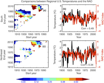
Figure 7 Comparisons between observed wintertime surface temperature and the NAO index for the southern U.S. (top) and northeast U.S. (bottom). (left) The ratio of temperature trends in the regressed NAO index (Hurrell and Deser 2009, NCAR Staff 2016) to the observed temperature trends. Time periods where the observed trend is insignificant are whited out. (right) The time series of the observed temperature anomalies (black) and the NAO index (red). All time series are anomalies with respect to 1901–2005.
Download figure:
Standard image High-resolution imageIn order to assess the role of SST forcing in driving winter temperature trends in the U.S., we examine a set of GOGA simulations that were performed with NCAR CAM5 (see section 2). An important side note when considering these simulations is that the SST trends used to drive the CAM5 model reflect the influences of external forcings such as anthropogenic aerosols, greenhouse gases, and volcanic eruptions, as well as internal variability. We find that while the GOGA simulations do not capture the full magnitude and spatial extent of the observed mid-century cooling over the U.S., they do produce negative temperature trends in the southern and eastern U.S. during this time period (figures 8(b) and (c), supplemental figure 6). The weaker magnitude of the mid-century cooling in the GOGA simulations may contribute to the lack of a warming hole in the southern U.S. in GOGA over the entire period, 1901–2005 (compare figure 2(a) and figure 8(a); see also supplemental figure 6). The GOGA simulations do not pinpoint which region(s) of the global oceans is driving the cooling trends, but the timing is consistent with the PDO as discussed previously (figure 6). We conclude that either the observed mid-century cooling is not entirely forced by the observed SST patterns, or that the model is not realistically representing the atmospheric response to SST changes.

Figure 8 Trends in wintertime surface air temperature (°C/decade) in the ensemble mean of the CAM5 GOGA simulations from 1901–2005 (left), 1950–1975 (center), and 1950–1990 (right).
Download figure:
Standard image High-resolution image
We further evaluate the role of atmospheric variability in the GOGA simulations by calculating the NAO index in each ensemble member. We find that the ensemble-average correlations between the NAO and regional temperature in the southern U.S. (r = 0.35) and northeast U.S. (r = 0.35) are realistic, although smaller than the observed relationship in the southern U.S. (r = 0.49). The ensemble mean captures some of the observed temporal features of the NAO index, including a negative trend between 1950–1970, and a positive trend between 1965–2005, but it does not capture the full magnitude of the observed negative trends (supplemental figure 7). This finding suggests that variability in the NAO may be partially SST forced and further that a portion of the significant observed cooling in the southern U.S. from 1950–1970 may reflect of modulation of the NAO by SST changes.
5. Conclusions
Prior studies attribute the United States 'warming hole' to internal variability in Atlantic and Pacific SSTs or to changes in external forcing from either anthropogenic aerosols or land use principally through their effects on rainfall, soil moisture, and cloud cover (see supplemental table 1). In this study, we reconcile these competing explanations by demonstrating the importance of considering the seasonality and temporal evolution of temperature trends when studying the U.S. warming hole as well as considering an additional mechanism, the NAO, which has not been investigated previously.
In summer, we find that both external forcing and internal variability are important for understanding the observed warming hole. Significant observed summertime cooling trends occur during 1950–1975 in the southern and northeast U.S. We find that anthropogenic aerosols are significant contributors to this cooling. This finding is in agreement with previous research by Yu et al 2014 who argued that aerosols were a significant driver of cooling trends in the eastern and southern U.S. from 1950–1985 through their effects on clouds. It is also consistent with the findings from Leibensperger et al 2012 who performed a time slice experiment simulating the 1970–1990 time period to show the potential aerosol impacts on temperature in the eastern and central U.S. through their effects on regional circulation patterns. Aerosol forcing over the U.S. diminishes after the mid-1970s (supplemental figure 3), and so studies that examined longer time periods of 50 or more years (Wang et al 2009, Meehl et al 2012, Weaver 2012, Pan et al 2013) or time periods starting in the 1980s or later (Robinson et al 2002) overlooked this effect.
While aerosols likely contributed to the observed summer warming hole, the full spatial pattern of temperature change, characterized by cooling in the southern and northeast U.S. and warming in the western U.S. (figure 1(c)), is likely shaped largely by internal variability. Wang et al (2009), Meehl et al (2012), and Weaver (2012) attribute the observed cooling in the second half of the twentieth century to heating anomalies in the eastern Pacific, associated with the PDO, while Weaver et al (2012) additionally highlights changes in North Atlantic SSTs affecting the strength of the Great Plains low level jet. Internal variability also drives the observed negative temperature trends in the north central and northeast U.S. beginning in the 1930s. These regions were strongly influenced by the anomalously warm Dust Bowl of that decade which was most likely caused by variability in Pacific SSTs (Schubert et al 2004, Seager et al 2008, Donat et al 2016).
Observed wintertime temperature trends are driven mainly by changes in internal modes of climate variability, with no evidence of a significant effect from aerosol forcing. We regress the observed PDO and NAO indices against the observed regional temperature record to determine the fraction of the observed temperature trends that can be explained by these modes. The PDO explains as much as half of the observed wintertime cooling over the southern U.S. during 1950–1990, supporting past studies linking the winter warming hole to Pacific SSTs (Robinson et al 2002, Wang et al 2009, Meehl et al 2012). The NAO, in contrast, which has not been examined in previous studies, is a better predictor of southern and northeast U.S. cooling from the 1940s and 1950s to the mid 1970s, explaining up to 50% of the observed temperature trends.
The NAO and the PDO may in turn be affected by external forcing. For example, Allen et al (2014) show that the CMIP5 multi-model mean captures the observed positive trend in the PDO from 1950–1979 and negative trend from 1979–2009, suggesting anthropogenic forcing is influencing this mode of variability. In particular, they find that forcing from anthropogenic aerosols can account for approximately two-thirds of the observed positive PDO trend from 1950–1979, which we associate with winter cooling in the southern U.S. (figure 6). Smith et al 2016 argue that Asian aerosols have influenced the PDO through their impacts on the Aleutian Low. Regarding the NAO, the large magnitude of interannual (unforced) variability makes detection and attribution of forced trends difficult. However, CMIP5 multi-model means project that the NAO index will increase over the twenty-first century in response to climate change (Gillett and Fyfe 2013), with some studies also suggesting that increasing (decreasing) anthropogenic aerosols may contribute to negative (positive) trends in the NAO (e.g. Chiacchio et al 2011, Pauseta et al 2015).
Observed temperature trends from the mid-1970s to the present are consistently positive across the U.S. in both winter and summer. In summer, these warming trends are likely due to the leveling off of global aerosol emissions and the decrease in U.S. aerosol emissions, in combination with the continued rise in greenhouse gas concentrations (see figure 3). Future emissions scenarios project continuing decreases in aerosol emissions (van Vuuren et al 2011), so we expect that multi-decadal periods with regional summertime cooling, such as observed during the twentieth century, will become less likely. In winter, the change in phase of the PDO and the NAO is most likely driving the reversal in U.S. temperature trends after the mid-1970s (Meehl et al 2015). The winter warming hole may recur when the PDO and/or NAO change phase again in the future.
Acknowledgments
We would like to thank our reviewers for their helpful feedback on this study, and our colleague Donna Lee, who performed the CAM5 GOGA simulations used in this research. This article was developed under Assistance Agreement No. 83520601 and 83587801 awarded by the U.S. Environmental Protection Agency to AMF. It has not been formally reviewed by the EPA. The views expressed in this document are solely those of the authors and do not necessarily reflect those of the Agency. Additionally, Mingfang Ting acknowledges support from NOAA Grant NA14OAR4310223. Lamont-Doherty Publication Number 8090.