


ABSTRACT
Since 2009, observations by the Interstellar Boundary Explorer (IBEX) have vastly improved our understanding of the interaction between the solar wind (SW) and local interstellar medium through direct measurements of energetic neutral atoms (ENAs), which inform us about the heliospheric conditions that produced them. An enhanced feature of flux in the sky, the so-called IBEX ribbon, was not predicted by any global models before the first IBEX observations. A dominating theory of the origin of the ribbon, although still under debate, is a secondary charge-exchange process involving secondary ENAs originating from outside the heliopause. According to this mechanism, the evolution of the solar cycle should be visible in the ribbon flux. Therefore, in this paper we simulate a fully time-dependent ribbon flux, as well as globally distributed flux from the inner heliosheath (IHS), using time-dependent SW parameters from Sokół et al. as boundary conditions for our time-dependent heliosphere simulation. After post-processing the results to compute H ENA fluxes, our results show that the secondary ENA ribbon indeed should be time dependent, evolving with a period of approximately 11 yr, with differences depending on the energy and direction. Our results for the IHS flux show little periodic change with the 11 yr solar cycle, but rather with short-term fluctuations in the background plasma. While the secondary ENA mechanism appears to emulate several key characteristics of the observed IBEX ribbon, it appears that our simulation does not yet include all of the relevant physics that produces the observed ribbon.
Export citation and abstract BibTeX RIS
1. INTRODUCTION
The Interstellar Boundary Explorer (IBEX) mission (McComas et al. 2009b) has provided us with invaluable measurements of energetic neutral atom (ENA) fluxes that arise as a consequence of the solar wind–local interstellar medium (SW–LISM) interaction. In particular, the so-called IBEX ribbon, a region of enhanced intensity encircling the sky (McComas et al. 2009a, 2010, 2012b), is a unique feature in the data. The first observations revealed that the ribbon was dominating the all-sky flux at a wide range of energies (∼0.2–6 keV; McComas et al. 2009a), with a brightness ∼2–3 times the globally distributed flux and an average width of ∼20° (Fuselier et al. 2009), approximately centered around ecliptic coordinates (221°, 39°) (Funsten et al. 2009b). A comparison to three-dimensional (3D) MHD simulations of the heliosphere suggested that the disturbed LISM magnetic field near the heliopause (HP) was perpendicular to the IBEX lines of sight (LOSs) to the ribbon, supporting mechanisms of the ribbon that relied on the ordering of the LISM magnetic field (Schwadron et al. 2009a). Below ∼0.2 keV, the dominating features in the sky were high concentrations of interstellar hydrogen (H), helium, and oxygen, with no ribbon structure visible (Möbius et al. 2009).
One possible explanation for the ribbon's existence is based on a secondary charge-exchange process, where ENAs from the supersonic and subsonic SW cross the HP, charge exchange to become pickup ions (PUIs) in the outer heliosheath (OHS), and charge exchange again into secondary ENAs that may be directed back inside the heliosphere, with higher intensity along directions perpendicular to the interstellar magnetic field (McComas et al. 2009a). Soon after the first observations, several global simulations of the secondary ENA mechanism produced results similar in both quality and quantity to the observations (Chalov et al. 2010; Heerikhuisen et al. 2010b), with more recent models showing similar results (Schwadron & McComas 2013b; Möbius et al. 2013; Isenberg 2014). While the secondary ENA mechanism appears to be the strongest candidate, many others have been suggested to explain its creation (see recent review by McComas et al. 2014b, and references therein), and the ribbon's true origins remain unresolved.
McComas et al. (2010) presented the first year of Compton–Getting-corrected IBEX data, which showed changes in flux over a period of 6 months. They reported a decrease in flux over most of the sky, in both the ribbon and globally distributed flux. In the ribbon region, the "knot," a small region of high emission, appeared to decrease in intensity and spread to lower and higher latitudes. Also, the southernmost portion of the ribbon appeared to move slightly northward. All of these changes may be due to the dynamic solar cycle, including small-scale fluctuations in the SW, the transition between fast and slow SW, and large-scale fluctuations near the HP (see, e.g., Pogorelov et al. 2009a, 2011, 2013).
Since IBEX spins around a Sun-pointing axis as it orbits the Earth (McComas et al. 2009b), it is able to detect ENAs from the directions of the ecliptic poles almost continuously, providing a unique opportunity to study the evolution of IBEX data on short timescales. Analyzing the first 2 yr of data, Reisenfeld et al. (2012) reported a significant, energy-dependent drop in flux measured by IBEX-Hi from the ecliptic poles, similar to earlier reports (McComas et al. 2010). They also analyzed the relationship between the outward propagation of SW and the inward propagation of H ENAs from the inner heliosheath (IHS) to estimate distances to the termination shock (TS) and HP in the north and south polar directions. Dayeh et al. (2012) analyzed the energy dependence of IBEX-Hi data from the south ecliptic pole direction over a similar range of time. They found that a spectral break in the data between ∼1 and 2 keV is likely due to a source of PUIs in the fast SW downstream of the TS, while at lower energies the spectra are likely generated from a PUI source from the slow SW. Furthermore, Dayeh et al. (2011) showed a clear correlation between IBEX spectra as a function of latitude and the fast/slow SW speeds measured by Ulysses (see Figure 4 in Dayeh et al. 2011). This suggests the importance of including fast and slow SW in 3D simulations of the heliosphere. Allegrini et al. (2012) also confirmed the continuous decline of flux over the first few years by correcting for the approximate time lag between ENA creation and detection, as a function of energy. Similar to previous studies, they found that flux from the poles has been decreasing over time.
McComas et al. (2012b) provided the first 3 yr of IBEX data, developing a more sophisticated model to correct for the survival probability of H ENAs out to 100 AU from the Sun. They reported a continuous, although slower, drop in flux over most of the sky from 2009 to 2011, with the strongest changes seen in the direction of the ribbon. More recently, McComas et al. (2014a) presented the latest IBEX data from 2009 to 2013. While they also show a continuation of the reduction in flux, the data show a slow-down in the decline of flux from certain areas of the sky. We will discuss implications of this observation with our results later in Section 3.3.
Over the past few decades there have been numerous models developed to study the influence of the dynamic SW ram pressure (density and velocity) on the global structure of the heliosphere, including short-term fluctuations ( 6 months) and the long-term solar cycle (∼11 yr). In the following discussion we focus our attention on models of quasi-periodic fluctuations in SW ram pressure, as related to this paper (such as the 11 yr solar cycle). For a list of early studies not included in this discussion, see, e.g., Barnes (1993, 1994), Suess (1993), Donohue & Zank (1993), Naidu & Barnes (1994a, 1994b), Story & Zank (1995), Ratkiewicz et al. (1996), and Pogorelov (2000).
Spurred on by Pioneer 10 and 11 (Barnes 1990) and Voyager 2 (V2, Lazarus & McNutt 1990) observations of short-term, large-scale fluctuations in the SW ram pressure, Belcher et al. (1993) used a one-dimensional (1D) kinematic model to study the effects of fluctuations in the SW ram pressure on the TS, showing significant modulation of the TS position, while Whang & Burlaga (1993) used a 1D MHD model to study the long-term (∼11 yr) effects on the TS, with results showing the distance to the TS to be periodic with the solar cycle. Steinolfson (1994) modeled a two-dimensional (2D) gasdynamic simulation of the SW–LISM interaction with a sinusoidally varying, short-term SW pressure, with results suggesting lower-amplitude oscillations in the TS position than those obtained in 1D, while with a similar model, Karmesin et al. (1995) found more significant motion of the TS in response to the 11 yr solar cycle, with disturbances propagating through the LISM. Pogorelov (1995) also studied the 2D case of the 11 yr solar cycle effect on a gasdynamic heliosphere, showing that the TS position was oscillatory, with a smaller effect on the HP and bow shock. Pauls & Zank (1996) studied the effects of a nonuniform SW (i.e., fast SW near the poles, slow SW near the ecliptic plane; Phillips et al. 1995) on a 3D, gasdynamic heliosphere, showing that the TS becomes elongated in the polar direction, and that the shocked SW mainly flows around the TS in the ecliptic plane, whereas Pauls & Zank (1997) showed that the inclusion of charge that exchange with interstellar neutrals reduced these asymmetries, providing insight into the global importance of charge exchange on the dynamical heliosphere. Barnes (1998) also illustrated, using an analytic approach, the dependence of TS position on latitudinal variations in SW ram pressure, indicating the behavior of unique positions of obliquity in the TS. Using an approach similar to Belcher et al. (1993), Richardson (1997) estimated the instantaneous response of the HP to long-term fluctuations in the SW ram pressure, suggesting a significant amount of motion compared to the LISM flow. Baranov & Zaitsev (1998) used a 2D gasdynamic simulation of the two-shock heliosphere to study its evolution in the 11 yr solar cycle, showing results similar to previous studies of significant modulation of the TS position, and less for the HP; however, they showed little variation for the bow shock. Wang & Belcher (1999) introduced uniform short- and long-term fluctuations in the SW ram pressure into their 2D gasdynamic simulation of the heliosphere, where the TS also moved significantly inward and outward due to the 11 yr solar cycle (however, again mediated by charge exchange with interstellar neutrals) and less significant for shorter timescales, and little reaction at the HP. Tanaka & Washimi (1999) developed a time-dependent, 3D MHD simulation of the SW–LISM interaction (although ignoring the effects of charge exchange), with uniform fast and slow SW parameters and a transition between these regions that varies over time, revealing a more complicated structure of the TS and IHS. Zank (1999), using a 2D, axially symmetric, time-dependent MHD model, included the effects of charge exchange while varying the SW ram pressure over an 11 yr cycle. They also found that the TS experienced relatively large modulation, although mediated by charge exchange, and the combination of time-dependent SW and Rayleigh–Taylor instabilities made the HP unstable. Zaitsev (2000) continued the work of Baranov & Zaitsev (1998) by including charge exchange with a quasi-stationary distribution of neutral H, finding more variability in the positions of the HP and bow shock. Scherer & Fahr (2003a, 2003c), and Zank and Müller (2003) included charge exchange in a time-dependent, axially symmetric simulation of the heliosphere, showing the effects of a uniformly varying SW ram pressure on the global structure, including a similar "breathing" effect on the TS, and to a smaller degree, the HP. Borrmann & Fichtner (2005) studied short- and long-term fluctuations in the SW, finding minimal variations in the TS position at low latitudes, and also introduced variable LISM conditions that act on the heliosphere over much longer times. Pogorelov et al. (2009a) included the effects of a uniformly varying transition between fast and slow SW over the 11 yr solar cycle in their 3D MHD simulation of the heliosphere, similar to Tanaka & Washimi (1999) except by including the effects of charge exchange with interstellar neutrals, as well as the tilt angle between the solar rotation and magnetic axes, where they analyzed the effects of the heliospheric current sheet on the supersonic SW. As shown in Pogorelov et al. (2009a) and further elaborated in Pogorelov et al. (2012), solar cycle effects may create long-lasting regions of sunward SW flow observed by Voyager 1 (V1; Decker et al. 2012).
With more in situ data from the outer reaches of the heliosphere from the Voyager spacecraft, models began to use these measurements to constrain their simulations even further. Izmodenov et al. (2008) included a more realistic solar cycle in their axially symmetric simulation in order to study the TS crossings of the Voyager spacecraft (Stone et al. 2005, 2008), with results suggesting the importance of including the solar and interstellar fields on studies of the TS asymmetry. Washimi et al. (2011) incorporated V2 measurements in time-sensitivity studies using a 3D MHD simulation of the heliosphere to fit to V1 and V2 TS crossings, while Strumik et al. (2011), Ben-Jaffel & Ratkiewicz (2012), and Ben-Jaffel et al. (2013) also used time-sensitivity studies, although assuming a constant H flux, to constrain the LISM magnetic field needed to fit the IBEX ribbon direction and V1, V2, and Advanced Composition Explorer measurements (see, e.g., McComas et al. 2013). Pogorelov et al. (2013) coupled Ulysses observations of the SW speed as a function of latitude (Ebert et al. 2009) to their 3D, time-dependent MHD simulation of the heliosphere, showing the dynamical effects of the recent decrease in SW ram pressure on the distance to the TS in the Voyager directions. Borovikov & Pogorelov (2014) showed that, due to the combination of a dynamic SW and Rayleigh–Taylor instabilities near the front of the heliosphere, the LISM plasma will experience significant intrusions into the IHS, providing a possible explanation for the crossing of the HP by V1 much sooner than expected (e.g., Gurnett et al. 2013).
It is apparent that the dynamic SW has a significant impact on the heliosphere. A question remains as to how much the dynamic SW will affect H ENA flux relevant to IBEX. Recent studies have investigated this issue. Izmodenov & Malama (2004a, 2004b) and Izmodenov et al. (2005) introduced a kinetic description for neutral H into their time-dependent, axially symmetric simulation of the heliosphere, with a sinusoidal 11 yr solar cycle, showing variability in interstellar H atom properties, as well as ENAs created in the IHS. Scherer & Fahr (2003b, 2003c) and Fahr & Scherer (2004) demonstrated how the complicated history of a dynamic solar cycle could affect line-integrated measurements of ENA fluxes, which also depends on the ENA energy. Using a 3D, gasdynamic heliosphere, Sternal et al. (2008) studied the effect of a time-varying, fast–slow SW transition on global H ENA flux measurements, showing temporal changes in the global flux related to the solar cycle. In their 3D MHD/kinetic simulation, Heerikhuisen et al. (2010a) assumed that parent ENAs born in the supersonic SW will attain a random velocity given by fast and slow SW measurements made by Ulysses, demonstrating how the ribbon flux, normally dominating at 1 keV for uniform slow SW boundary conditions, may spread to higher energies. Heerikhuisen et al. (2012) computed H ENA flux from an idealized, time-dependent heliosphere, although assuming instantaneous ENA propagation to the detector, with results suggesting that the variability seen in the observed ribbon knot may be due to changes in the SW energy at high latitudes as the solar cycle transitions from minimum to maximum. Recently, Siewert et al. (2014) also analyzed the transit-time delays between the transport of SW plasma from the Sun through the IHS and detection of H ENAs at 1 AU, where changes in the solar cycle should be seen in measurements of ENA flux from the IHS within a few years, particularly for IBEX-Hi energies.
While there have been several analyses of the effects of the time-dependent SW on the IBEX ribbon (McComas et al. 2010, 2012b, 2014a), there have been no dedicated studies on simulating the time-dependent effects of the SW on the secondary ENA ribbon (however, see Heerikhuisen et al. 2010a, 2012 for simplified models). If the secondary ENA mechanism is responsible for creating the IBEX ribbon, then the SW evolution should be mirrored in secondary ENAs, to some degree. In order to determine the effect of the solar cycle on the evolution of the secondary ENA ribbon, as well as the IHS flux, in this paper we provide results from simulations of time-dependent H ENA flux during the epoch of IBEX observations. Due to the long delays in time between parent ENA creation in the SW and secondary ENA detection at 1 AU, we also offer predictions for the flux up through 2017.5. First, we show the method of simulation in Section 2. Second, we present results of simulating time-dependent H ENA flux between 2005.5 and 2017.5 in Section 3, discuss temporal features in the results, and compare them to observations. Finally, we conclude the discussion of the results and offer insights into their implications for IBEX observations, as well as our understanding of the time-dependent heliosphere, in Section 4.
We stress that the results presented in this paper assume that the IBEX ribbon is formed by the secondary ENA mechanism. Therefore, when discussing the simulation results, we use the term "secondary ENA ribbon" as the case in which one assumes that the IBEX ribbon is formed by the secondary ENA mechanism.
2. METHOD OF SIMULATION
A flowchart of the simulation process is shown in Figure 1. The process consists of two main steps: (1) simulating a time-dependent heliosphere (left, blue), and (2) computing time-dependent H ENA fluxes at 1 AU (right, red). The results from the heliosphere simulation are used as input in the ENA flux computations, which are interpolated as a function of space and time. We describe the heliosphere simulation in Section 2.1 and the ENA flux computations in Section 2.2.
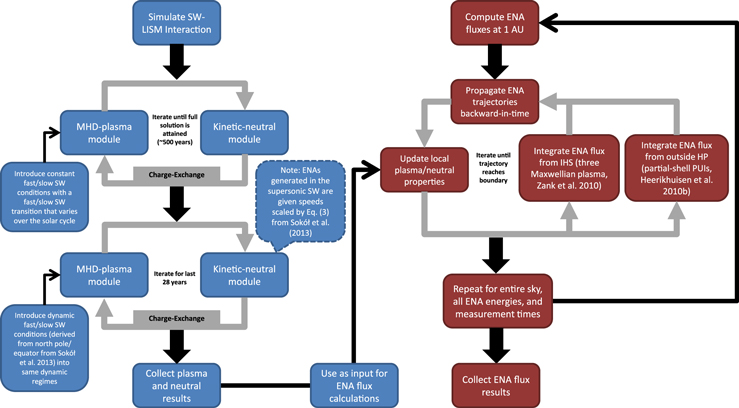
Figure 1. Flowchart of the simulation process. The MHD/kinetic simulation of the SW–LISM interaction is shown on the left (blue boxes), and the ENA flux simulation at 1 AU is shown on the right (red boxes). First, the SW–LISM interaction is simulated using our coupled MHD-plasma/kinetic-neutral modules. The first step is to simulate the heliosphere using ideal boundary conditions (Pogorelov et al. 2009a; constant SW speeds and densities in fast/slow SW regimes, whose boundary oscillates every 11 yr) until a full solution is attained. Then, time-dependent values for SW speed and density derived from two specific latitudes (north pole and equator) from Sokół et al. (2013) are introduced into the same fast/slow SW regimes from the previous step. During the kinetic-neutral iteration in the last 28 yr of the MHD/kinetic simulation, ENAs generated in the supersonic SW are given speeds as a function of latitude scaled by results from Sokół et al. (2013) (see Section 2.1.1). Once the heliosphere is simulated (i.e., we have 3D plasma and neutral data sets every 0.25 yr), the results are used as input for the ENA flux calculations. The MHD/kinetic results are interpolated as a function of space and time to compute ENA fluxes at 1 AU until the entire sky is mapped, for all energies and measurement times.
Download figure:
Standard image High-resolution image2.1. Simulating a Time-dependent Heliosphere
Before computing time-dependent ENA flux at 1 AU, we first simulate the SW–LISM interaction using a 3D, time-dependent, MHD-plasma/kinetic-neutral code (see Heerikhuisen et al. 2013, and references therein) based on the Multi-Scale FLUid-Kinetic Simulation Suite (MS-FLUKSS; Pogorelov et al. 2008b, 2009a). This assumes a single plasma fluid coupled with a kinetic description for neutral H through mass, momentum, and energy source terms. The equations used to simulate the 3D, time-dependent SW–LISM interaction are shown in the Appendix. During charge-exchange events, the IHS plasma is assumed to be a generalized-Lorentzian, or "kappa," distribution ( ), and Maxwellian elsewhere. This approximates the total energy of the IHS plasma, with the core of the distribution representing the cool SW, and the high-energy tail for PUIs and suprathermal ions (e.g., Heerikhuisen et al. 2008). However, it is important to note that we assume that the value of κ remains constant in the MHD/kinetic simulation and therefore may not accurately describe the evolution and relative proportions of the plasma distribution in the IHS. The incorporation of a self-consistent description of the IHS plasma is left for future studies.
2.1.1. Implementation of Dynamic SW Boundary Conditions
For every iteration of the MHD-plasma code, the SW inner boundary conditions are updated based on a dynamic solar cycle. First, we assume that the SW boundary conditions follow an idealized solar cycle, similar to Pogorelov et al. (2009a), where the transition between fast and slow SW varies sinusoidally with an 11 yr period, the transition approaches ±35° at solar minimum and ±80° at solar maximum, the current sheet tilt angle goes from 0° at minimum to 90° at maximum, the magnetic field polarity reverses at solar maximum, and the fast and slow SW speeds (800 and 400 km s−1, respectively) and densities (3.6 and 8 cm−3, respectively) are held constant. Between each iteration of the MHD-plasma code, the kinetic-neutral code is also run, coupling the neutral H atoms to the evolving plasma through source terms (see Appendix). The coupled MHD/kinetic code is run for a sufficiently long time to produce a full, time-dependent solution of the heliosphere and to fill the IHS with material from previous solar cycles. In practice, the simulation runs for more than 500 yr, such that the slow LISM plasma and neutrals have sufficient time to interact with the heliosphere and propagate through the simulation domain.
For the last 28 yr of the simulation, we use new, time-dependent values for the fast and slow SW speeds and densities. These values, beginning at solar maximum in 1990.5 (see Figure 2), are introduced into the simulation initially at a time corresponding to solar maximum in the simulation. The SW boundary conditions are then updated at every iteration of the simulation for the next 28 yr, as shown in Figure 2. These boundary conditions are calculated from time- and latitude-dependent functions of SW speed and density from Sokół et al. (2013), which are based on line-integrated interplanetary scintillation and in situ measurements of the SW, scaled to 1 AU. We take values for the SW speed and density at heliolatitudes of 0° (equator) and +90° (north pole) using Equations (3) and (4) from Sokół et al. (2013), as a function of time, and use these for the SW boundary conditions for the slow and fast SW regimes, respectively (see Figure 2). We assume that the fast and slow SW still maintain uniform speeds and densities at the inner boundary, in their respective regions, although varying as a function of time. The transition between fast and slow SW, the current sheet tilt angle, and magnetic field polarity still vary according to the method from Pogorelov et al. (2009a). The MHD-plasma and kinetic-neutral codes continue to iterate in order to couple the neutral H with the plasma. These last 28 yr correspond to times between 1990.5 and 2017.5, during which we compute H ENA fluxes at 1 AU in the post-process step (Figure 1, red boxes), which is described in Section 2.2.
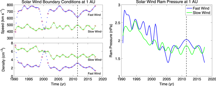
Figure 2. Time-dependent solar wind boundary conditions at 1 AU (left) used for the last 28 yr of the MHD/kinetic simulation, derived from Equations (3) and (4) from Sokół et al. (2013). We use values from the equatorial plane (0° latitude) for the slow SW region and from the north pole (+90° latitude) for the fast SW region. The red stars are yearly averaged values from Sokół et al. (2013), and the blue/green dots are values interpolated between the yearly averages using a cubic spline. On the right is the SW ram pressure at 1 AU ( ), calculated from the values from the left panel. Since the range of data provided by Sokół et al. (2013) is between 1990.5 and 2011.5, we reverse the fast and slow SW profiles after 2011.5 (vertical dashed lines) to provide us with a background, time-dependent heliosphere up to 2017.5.
Download figure:
Standard image High-resolution imageIt would be ideal to incorporate the full latitudinal profile of Equations (3) and (4) from Sokół et al. (2013) as boundary conditions in our MHD/kinetic simulation. However, since we connect the last 28 yr of the simulation (with dynamic boundary conditions; see Figure 2) to the simplified solar cycle with a fast/slow SW transition that varies sinusoidally with an 11 yr period, we resort to the boundary conditions discussed above in order to preserve this frequency. This method, however, may not provide the most realistic distribution of ENAs produced in the supersonic SW, which is important for the secondary ENA mechanism. Therefore, we can improve the ENA distribution in the supersonic SW by scaling the speeds of those ENAs generated in our kinetic-neutral module by the latitude-dependent speeds from Equation (3) of Sokół et al. (2013). For example, an ENA generated in the supersonic SW in our kinetic-neutral module is given a speed calculated by  , where
  is the speed determined by Equation (3) from Sokół et al. (2013),
  is the local speed at position r determined by charge exchange with the MHD plasma, and
  is the speed determined by charge exchange with the MHD plasma at 1 AU, all at the same latitude θ. This method was also used by Heerikhuisen et al. (2010a, 2012, 2014) and Zirnstein et al. (2013), providing a simple way to improve the latitudinal spectrum of the secondary ENA ribbon, while also taking into account the slowing of the supersonic SW due to the incorporation of PUIs. The probability for the charge-exchange event to occur, however, is still self-consistently determined by the local plasma properties from the MHD/kinetic solution of the heliosphere. Elsewhere in the heliosphere (IHS, OHS, and LISM), the speeds of newly created ENAs are self-consistently determined from the local plasma properties.
The data taken from Sokół et al. (2013) only span from 1990.5 to 2011.5; therefore, we must estimate the SW boundary conditions beyond 2011.5 in order to provide us with a background heliosphere for which to self-consistently calculate ENA flux from, beyond 2011.5. First we notice that the slow SW speed has, on average, remained fairly constant since 1990.5 (although with quasi-periodic oscillations around the mean). Therefore, for the slow SW speed beyond 2011.5 we reverse the profile from 2011.5 to 2006 and substitute it for the profile for 2011.5 to 2017.5. For example, the slow SW speed in 2011.75 is the same as 2011.25, 2012 is the same as 2011, etc. Although the slow SW density has decreased from 1990.5 to ∼2005, it has remained fairly constant since then. Therefore, we do a similar reversal for the slow SW speed.
The fast SW speed and density, however, are more complicated. As the solar cycle approaches maximum, the speed (density) near the poles decreases (increases) closer to the slow SW value as the coronal holes close. However, we again choose to reverse the profile of fast SW speed and density beyond 2011.5, for the following reasons. First, since the latest solar maximum was significantly different from the previous maximum, we can not accurately predict the fast SW behavior. Second, the maximum (minimum) in fast SW density (speed) during the previous solar maximum occurred in ∼2000.5, which is a full cycle before 2011.5, suggesting that a reversal at 2011.5 would be sufficient. Third, while we may assume some form of the fast SW profiles beyond 2011.5, we do not need accurate SW boundary conditions beyond 2011.5 to predict the ribbon flux for the next ∼3.5–9.5 yr, which will be discussed in more detail in Section 3.3. Therefore, for the sake of simplicity we reverse the profiles in 2011.5 as was done for the slow SW. The point of reversal for slow and fast SW in 2011.5 is indicated by the vertical dashed lines in Figure 2.
2.1.2. Implications of SW Boundary Conditions
We note that it takes time for the new boundary conditions taken from Sokół et al. (2013) to propagate through the simulation domain, and this may have adverse effects on our ENA flux results. Therefore, we consider its potential impact in a few simplified cases. The earliest time that we simulate flux at 1 AU is 2005.5 (see Figures 15, 16, 19, 20). For ENAs in the lowest IBEX-Hi energy passband, with energy ∼0.71 keV and speed ∼369 km s−1 (the center of passband 2), the time it takes to propagate from 1000 to 1 AU is ∼12.9 yr, from 200 to 1 AU is ∼2.6 yr, and from 100 to 1 AU is ∼1.3 yr. Assuming reasonable values for the SW speed (400 km s−1 upstream, 100 km s−1 downstream in the tail direction, and 50 km/s downstream in the nose direction) and TS distance (90 AU upwind, and 140 AU downwind), the SW plasma takes ∼42 yr to propagate from 1 AU down the heliotail to the simulation boundary, and ∼4.9 yr to propagate to the HP in the upwind direction (∼130 AU). Therefore, the plasma in the heliotail is not completely filled with the new SW conditions from Sokół et al. (2013) before we begin computing ENA fluxes at 1 AU (in 2005.5). Near the front of the heliosphere, however, there is a sufficient amount of time to fill the IHS before we begin H ENA flux computations.
However, plasma flowing toward the front of the heliosphere is slowed and diverted near the HP and takes a longer amount of time to flow to the poles and flanks and down the heliotail. Based on estimates of the transit times of SW through the IHS up to ENA detection from the poles (Dayeh et al. 2014; Siewert et al. 2014), we estimate a maximum transit time of ∼15 yr in the front half of the heliosphere. Since we compute flux after 2005.5 (at least 15 yr after introducing the new SW boundary conditions), our IHS flux results from the front of the heliosphere remain largely unaffected by the initial SW boundary conditions. However, near the downwind direction, our results may potentially include some ENAs generated by plasma from before the introduction of the SW boundary conditions from Sokół et al. (2013).
For the majority of the ribbon flux, the total time it takes to detect a secondary ENA from past SW conditions ranges between ∼3.5 and 9.5 yr, depending on the distance to the ribbon source and the ENA energy (see Section 2.2.2 and Table 2). Also, the amount of time it takes for the SW to fill the region upstream of the TS, which produces the majority of primary ENAs that fuel the secondary ENA ribbon, is approximately 1 yr. Therefore, we conclude that our simulated ribbon results, beginning in 2005.5 (15 yr after the introduction of SW boundary conditions from Sokół et al. 2013), are generally unaffected by the change in SW boundary conditions.
As discussed in Section 2.1.1, ENAs generated in the supersonic SW in the kinetic-neutral model during the last 28 yr of the MHD/kinetic simulation are given speeds scaled by the latitude and time-dependent results from Sokół et al. (2013). While this method is not initially self-consistent with the MHD/kinetic simulation, the resulting ENAs are still coupled to the MHD plasma by charge exchange. This method provides (1) a more realistic outward-propagating, neutralized, supersonic SW distribution; (2) more realistic heating in the OHS plasma by charge exchange; and (3) more realistic secondary ENA spectra. However, we note that this method does not include the convection time of SW from 1 AU to the location at which a new ENA is generated in the supersonic SW, which may introduce (1) a ≲0.5 yr (on average) discrepancy in our results, and (2) the ratio  may vary between ∼0.5 and 2 when computed near the fast/slow SW transition (e.g., when the SW at distance r from the Sun is slow [fast], and the SW at 1 AU, at the same point in time, is fast [slow]). While the effects of these simplifications have not been quantified, we note that (1) the resolution of our ENA flux results presented in Section 3 is 1 yr, and thus we do not expect a significant uncertainty when analyzing the evolution of ENA flux over multiple years; and (2) the fast/slow SW transition region is narrow most of the time and likely only affects a small portion of the outward-propagating, supersonic ENA flux.
Since there is a considerable delay in time between parent ENA creation in the supersonic SW and secondary ENA measurement at 1 AU (between ∼3.5 and 9.5 yr; see Table 2), we are able to predict ribbon flux consistently up until ∼2015–2021, depending on the energy of the ENA and the direction. Flux from the IHS, however, cannot be accurately predicted more than a few years into the future. Therefore, one must keep in mind that our results presented later in the paper for the IHS flux depend strongly on our assumptions of the SW boundary conditions beyond the currently available data.
2.1.3. Implementation of Static LISM Boundary Conditions
The LISM boundary conditions for our time-dependent MHD/kinetic simulation are shown in Table 1, which we assume do not vary over the timescale of the simulation. The LISM plasma temperature (T), velocity (u), and magnetic field strength (B) were chosen based on consensus values derived from Schwadron et al. (2011), Möbius et al. (2012), Bzowski et al. (2012), and McComas et al. (2012a). The plasma and neutral densities were chosen in order to constrain the TS position to approximately agree with Voyager observations (although our simulation is not accurate enough to reproduce the time-dependent asymmetry of the V1 and V2 crossings), as well as to produce an H atom density at the nose of the TS of ∼0.09 cm−3.
Table 1. LISM Boundary Conditions
| Parameter | Value | Reference |
|---|---|---|
| T (K) | 6200 | 1,2 |
| np (cm−3) | 0.07 | ⋯ |
| nH (cm−3) | 0.18 | ⋯ |
| u (km s−1) | 23.2 | 1–3 |
| B (μG) | 3 | 4 |
 (ecliptic J2000) (ecliptic J2000) |
(79°, −5°) | 1–3 |
 (ecliptic J2000) (ecliptic J2000) |
(45°, −44°) | ⋯ |
References. (1) Möbius et al. (2012); (2) Bzowski et al. (2012); (3) McComas et al. (2012a); (4) Schwadron et al. (2011).
Download table as: ASCIITypeset image
From the mathematical perspective, we use characteristics-based boundary conditions at the outer boundary with additional modifications described by Pogorelov & Semenov (1997).
2.1.4. Implications of LISM Boundary Conditions
A recent study that looked at the trend of the interstellar He flow direction through the heliosphere, inferred from multiple sources of measurements over the past 30 yr, reported that a linear fit to the flow's ecliptic longitude direction shows a statistically significant increase over time (Frisch et al. 2013). However, we cannot accurately predict the evolution of the LISM conditions, and we assume that they vary slowly enough to not affect H ENA fluxes over the timescales presented in this paper.
There have been studies (see, e.g., Pogorelov et al. 2007, 2008a, 2009b, 2013; Richardson et al. 2008; Izmodenov 2009; Opher et al. 2009; Washimi et al. 2011) that have used modeling to constrain the interstellar magnetic field strength and direction needed to explain the asymmetry of the TS inferred by the Voyager spacecraft crossings (Stone et al. 2005, 2008), while other models have included a fit to the direction toward  outside the HP to the IBEX ribbon (see, e.g., Grygorczuk et al. 2011; Strumik et al. 2011; Ben-Jaffel & Ratkiewicz 2012; Ratkiewicz et al. 2012; Ben-Jaffel et al. 2013). The significance of the
  surface in the generation of the IBEX ribbon was identified during initial IBEX observations (McComas et al. 2009a; Schwadron et al. 2009a), based on correlations between the ribbon direction and the
  surface outside the HP (Pogorelov et al. 2009b, 2009c). In this paper we choose the strength and direction for
  based on recent analyses that fit simulations of the IBEX ribbon flux using the secondary ENA mechanism to the observed ribbon (Heerikhuisen & Pogorelov 2011; Funsten et al. 2013; Heerikhuisen et al. 2014), which are in general agreement with other studies that fit the IBEX ribbon to directions near
  .
.
In these simulations we use an older estimate for the interstellar magnetic field direction, coming from (225°, 44°), rather than aligned with the more recent value from Funsten et al. (2013). Since it will take a considerable amount of time for any changes to the LISM boundary conditions to propagate through the entire computational grid, and the simulations require a significant amount of computational time, we use this older estimate for the LISM magnetic field in this paper, rather than assuming that the center of the ribbon is aligned with the interstellar field direction. Therefore, the direction of maximum flux from our simulated ribbon is slightly different from the observed ribbon, partially due to this difference. Heerikhuisen et al. (2014) also showed that the simulated ribbon center is offset from the simulated, pristine interstellar field direction by a few degrees, depending on the strength of the interstellar magnetic field (also see Grygorczuk et al. 2011). However, for the purposes of this paper, we only require an approximate direction for the interstellar magnetic field, such that the directions toward  , and thus the simulated ribbon, approximately coincide with the IBEX ribbon.
Recent V1 measurements of anomalous and galactic cosmic rays (Webber & McDonald 2013; Krimigis et al. 2013; Stone et al. 2013), as well as (indirectly) plasma density (Gurnett et al. 2013), have indicated that the spacecraft is outside the HP. However, initial measurements of the interstellar magnetic field orientation showed little change from a Parker spiral (Burlaga et al. 2013), although recent measurements of the field direction indicate a larger deviation (Burlaga & Ness 2014). Many studies have followed to explain these observations (Krimigis et al. 2013; Swisdak et al. 2013; Fisk & Gloeckler 2013, 2014; Florinski et al. 2013; Opher & Drake 2013; Schwadron & McComas 2013a; Borovikov & Pogorelov 2014; Gloeckler & Fisk 2014; Strumik et al. 2014). While the thickness of the heliosheath suggested by the recent crossing is smaller than in our simulation, the evolutionary trends in our ribbon results will be largely unaffected. We will discuss this further in Section 4.
2.1.5. Time-dependent Heliosphere Results
In Figure 3 we show cross sections of plasma density computed using our time-dependent, 3D MHD/kinetic code, taken during solar minimum (left) and solar maximum (right). Notice the features similar to Pogorelov et al. (2009a), such as the transition between fast and slow SW near ±35° at solar minimum and ±80° at solar maximum, the sectored fast and slow SW densities in the heliotail, and the fluctuations in plasma density propagating through the OHS. We will discuss the effects of these fluctuations on the simulated ribbon flux in Section 4.
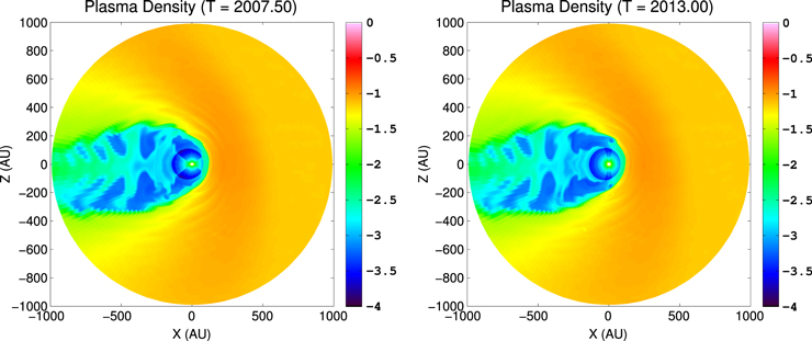
Figure 3. Cross section of plasma density (in units log10(cm−3)) in the Sun's polar plane, at a snapshot during solar minimum (2007.5, left) and solar maximum (2013.0, right).
Download figure:
Standard image High-resolution image2.2. Computing Time-dependent H ENA Fluxes
We simulate the measurements of time-dependent H ENA flux at 1 AU by integrating the time-dependent, differential H ENA flux equations (see Sections 2.2.4 and 2.2.5) along H ENA trajectories from 1 AU to the simulation LISM boundary (1000 AU). We approximate the H ENA trajectories by assuming that they are radial, straight lines from a Sun-centered origin, ignoring gravitational and radiation pressure effects. This approximation is valid for energies above ∼0.1 keV (see, e.g., Zirnstein et al. 2013) and thus a good approximation for IBEX-Hi energies. We integrate the H ENA flux equations for a discrete set of ENA energies within IBEX-Hi energy passbands 2–6 (McComas et al. 2012b) and then weight the contribution of the flux at each energy in the passband using the IBEX-Hi energy responses (Schwadron et al. 2009b). We also apply a simplified angular response function (Funsten et al. 2009a; Zirnstein et al. 2013), which tends to smooth out sharp features in the all-sky maps.
The flux equations are integrated along the trajectories such that, over a small period of integration time  , we calculate the accumulation of flux along the radial step
  , where
  , and v is the speed of the H ENA. At each step along the trajectory, we interpolate the MHD/kinetic simulation results (i.e., plasma and neutral properties) as a function of space and time in order to compute the accumulation of flux across that step. For example, at a distance l away from the spacecraft on an H ENA trajectory that intersects with IBEX, we calculate the accumulation of flux from the plasma and neutral conditions at a time
  in the past, where
  is the time of measurement and
  is the time for an H ENA to propagate to the spacecraft. This will be discussed in more detail in the following sections.
2.2.1. ENA Propagation Time
The flux simulation starts at the time of measurement at 1 AU,  , and integrates backward in time along the H ENA trajectory based on the speed of the H ENA we wish to simulate. The time of creation of an H ENA that will later be detected by the spacecraft is determined by the propagation time between the creation point and the spacecraft position. A primary H ENA from the IHS that is detected at 1 AU will travel anywhere from ∼90 (i.e., from the nose of the TS) to >1000 AU (i.e., from the extended heliotail), depending on the source location. For example, primary H ENAs with energies between ∼0.71 and 4.29 keV (corresponding to the nominal energies for IBEX-Hi passbands 2 and 6, respectively) will take between 1.16 and 0.47 yr for 90 AU and 12.9 and 5.23 yr for 1000 AU (we stress that these are only examples, not constraints in our simulations). However, as the SW flows away from the TS into the distant heliotail, high-energy PUIs that form a significant parent population for the ENA flux measured by IBEX-Hi will likely charge exchange within a few hundred AU from the TS (see, e.g., Zirnstein et al. 2014, Figure 3), thus reducing the effective time of propagation for the majority of high-energy ENAs from the IHS that are detected by IBEX. The time it takes the parent proton to advect with the plasma from the Sun to the position in the IHS before charge exchange occurs is an important characteristic for H ENA measurement and modeling (see, e.g., Allegrini et al. 2012; Reisenfeld et al. 2012; Dayeh et al. 2014; Siewert et al. 2014), and it is self-consistently accounted for in the MHD/kinetic simulation.
Secondary H ENAs with energies between ∼0.71 and 4.29 keV that propagate from the OHS (∼200 AU) to the spacecraft will take between ∼2.6 and 1 yr to travel to the spacecraft, respectively. However, secondary ENAs originally come from primary ENAs that crossed the HP, produced by charge exchange in the SW upstream or downstream of the TS. The propagation of these primary ENAs to the OHS is also taken into account in the MHD/kinetic simulation, and the propagation of secondary ENAs to 1 AU is taken into account in the post-process simulation.
2.2.2. PUI Charge-exchange Time
As stated earlier, primary and secondary ENAs both have intrinsic propagation times that depend on the distance between their source location and the detector. However, we must also take into account the delay time between the creation of PUIs in the OHS and the creation of the secondary H ENAs (which form the ribbon). This is a considerable amount of time for all energies relevant for IBEX.
In Table 2 we show estimates of the times relevant to the production and detection of secondary ENAs from outside the HP, for the benefit of the reader. We stress that for our simulations we directly calculate the time-dependent flux as a function of space and time and do not use the values shown in Table 2. For the nominal energy in each IBEX-Hi passband we provide estimates of the mean free path of ENAs traveling through the OHS, the charge-exchange time for PUIs at the same energy, and the total time between parent ENA creation (i.e., approximately the time in the solar cycle that created the parent ENA) in the supersonic SW and secondary ENA detection at 1 AU.
Table 2. Estimates of Time Delay between Parent ENA Creation and Secondary ENA Measurement
| Energy (keV) | ENA Mean Free Path in OHS (AU) | PUI Charge-exchange Time in OHS (yr) | Total Time Delay (yr) |
|---|---|---|---|
| 0.71 | 375–509 | 1.91–2.69 | 6.66–9.17 |
| 1.11 | 420–570 | 1.71–2.41 | 5.70–7.84 |
| 1.74 | 473–642 | 1.54–2.17 | 4.90–6.74 |
| 2.73 | 538–730 | 1.40–1.97 | 4.25–5.85 |
| 4.29 | 617–838 | 1.28–1.80 | 3.72–5.12 |
Notes. The ranges correspond to different directions through the OHS, during 2009.5. For the lower bound estimates, we assume that the OHS plasma density is 0.095 cm−3, the neutral density is 0.24 cm−3, and the distance to the HP is 130 AU. These correspond to the OHS properties in the direction toward the middle of the ribbon (see Figures 14 and 17). For the upper bound estimates, we assume that the OHS plasma density is 0.07 cm−3, the neutral density is 0.17 cm−3, and the distance to the HP is 170 AU. These correspond to the OHS properties in the direction of the north portion of the ribbon (see Figures 14 and 17). These densities are taken approximately 75 AU outside the HP (see Figure 17), since most ENAs visible at 1 AU originate from within ∼50 to 100 AU outside the HP, at least for 1.1 keV (Heerikhuisen & Pogorelov 2011). We estimate the propagation time outside the HP by assuming that it corresponds to traveling a distance 1/5 of the mean free path (since 1/5 of the mean free path for 1.11 keV is between ∼84 and 114 AU, which contains the majority of accumulated flux; Heerikhuisen & Pogorelov 2011). The total propagation time assumes that the parent ENA was created 40 AU from the Sun, in the direction of the middle (lower bound) or north (upper bound) ribbon directions. We emphasize that the estimates presented in this table are not assumed in our simulations, but are only meant to provide insight to the reader.
Download table as: ASCIITypeset image
As one can see, the time in the past that determined the energy and distribution of secondary ENAs ranges between ∼3.5 and 9.5 yr (for the majority of flux), largely depending on the energy of the ENA/PUI, the distance to the HP, and the OHS plasma and neutral properties. Although the parameters shown in Table 2 are not used in our simulations and are actually more complicated (for a space- and time-dependent heliosphere), these estimates are meant to assist the reader later in the paper.
While the source of PUIs that create secondary ENAs at a particular point in space and time extends from 0 to  into the past, this is computationally unfeasible to simulate. However, within three times the mean charge-exchange time, approximately 95% of the source of PUIs are accounted for. Therefore, the flux of secondary ENAs created at a particular point in space and time is approximately determined by a source of PUIs from a time 0 to 3
 in the past, where

is the mean charge-exchange time (when only 1/e particles have not experienced charge exchange yet), nH is the background H density, v is the PUI velocity (i.e., the ENA velocity, which we assume is much greater than the bulk neutral speed), and  is the energy-dependent, charge-exchange cross section (Lindsay & Stebbings 2005).
Figure 4 shows the (normalized) probability of PUIs, as a function of time in the past, to be the source of secondary ENAs, for energies 0.71 and 4.29 keV, assuming that the flux of secondary ENAs is created at time 0. We calculate the total flux of secondary ENAs at time 0, at a specific location in the OHS, by integrating the flux of secondary ENAs created over the interval 0 to 3 in the past (i.e., creating secondary ENAs from parent primary ENAs over a range of time in the past), and we weight the contribution of flux over the interval by an exponential function of the mean charge-exchange time (see Equation (4)). The majority of secondary ENAs created at time 0 will originate from parent primary ENAs that charge exchanged within three times the mean charge-exchange time in the past (vertical dashed lines), where the mean charge-exchange time is a function of energy and neutral density (assumed to be 0.2 cm−3 for the example shown in Figure 4). For smaller energies, the charge-exchange time is longer, and thus we integrate over a longer time. Higher-energy PUIs charge exchange more frequently, therefore only requiring a shorter integration time.
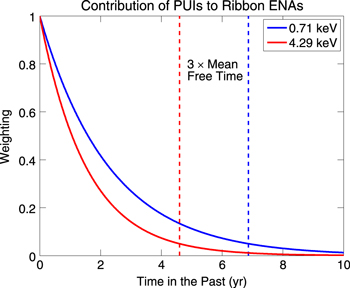
Figure 4. Contribution of PUIs as the source of secondary ENAs as a function of time, assuming that the fluxes of secondary ENAs are created at time 0. The weighting of PUIs created at some time in the past is an exponential function of the mean charge-exchange time, where we show the weighting for 0.71 (blue) and 1.11 (red) keV PUIs, assuming nH = 0.2 cm−3. The dashed lines represent the limit of our integration, which accounts for ∼95% of PUIs that would contribute to a flux of ENAs at time 0. Note that the integrals of the weightings shown in this figure do not equal 1.
Download figure:
Standard image High-resolution imageIn order to test whether only accounting for PUIs within three times the mean charge-exchange time in the past is sufficient, we compared our results to simulations of ribbon flux at 2009.5 that accounted for up to only twice the mean charge-exchange time for each energy. In directions toward the ribbon, i.e., near  , and in particular the directions where we focus our analysis of the ribbon (see Figure 14, north, middle, and south), the percent difference between these two simulations was approximately within ±10%. In certain regions of the sky away from the ribbon, the deviations reached up to ±20–30% depending on the energy and direction, which is likely due to (1) areas of low accumulated flux, (2) rapid variations over time, or (3) low OHS neutral H densities (which will increase the mean charge-exchange time). Unfortunately, computational limitations prevent us from simulating the case for four times the mean charge-exchange time, since this amount of time will likely exceed the maximum time range of plasma-neutral results allocated in our post-process simulation. However, since the errors of our current simulations compared to a more accurate one can only be smaller than the errors reported above, we do not expect our approximations to significantly affect the results presented in this paper.
When we calculate the mean charge-exchange time, the variables from Equation (1) are determined at the time of secondary ENA creation,  (i.e., at time 0 in Figure 4), although it should be integrated as a function of time into the past, from t = 0 to
  . However, first we assume in Equation (1) that the relative speed of charge exchange is dominated by the PUI speed such that uH and
  , and that the PUI speed remains constant. Second, we assume that the bulk neutral density outside the HP remains nearly constant over the charge-exchange time period. Although not shown, we computed the deviation in the bulk neutral density in the OHS, over an 11 yr period near the middle of the ribbon, and found that the maximum deviation is approximately ±2% and drops to less than 1% over a 2 yr period. Thus, this assumption will have little impact on our results. Therefore, the mean charge-exchange time remains nearly constant over these periods of time, outside the HP, and only varies as a function of space.
2.2.3. Motion of PUIs before Charge Exchange
Before charge exchange occurs, PUIs may stream along the interstellar magnetic field, depending on their initial pitch angle and the level of scattering. However, we ignore the effect of PUI streaming. Close to the ribbon, the parallel velocity (along the magnetic field) of PUIs is relatively small. For example, for a 1 keV PUI with an initial pitch angle of 80°, the parallel velocity (ignoring pitch-angle scattering) is ∼76 km s−1. Over the course of 2 yr before charge exchange, the PUI will move ∼32 AU, which corresponds to a maximum angular spread of ∼9° (depending on  ) as viewed from 1 to 200 AU, which is only slightly larger than the IBEX field of view (∼7°). If we include pitch-angle scattering, this may inhibit streaming if they scatter across 90°. Therefore, within the majority of the ribbon width of 20°, the movement of PUIs parallel to the interstellar field is not noticeably visible. However, this will be larger for faster PUIs, farther away from the ribbon, or if PUIs scatter to larger pitch angles, which may explain the large ribbon width at high energies (see, e.g., McComas et al. 2012b; Schwadron & McComas 2013b). On the other hand, PUIs with large pitch angles (assuming they do not scatter) will not be visible by IBEX, and therefore should not significantly affect our simulation results.
In their simulation of the ribbon, Chalov et al. (2010) assumed the no-scattering limit, allowing PUIs to stream along field lines until charge exchange occurred. In this limit, the magnetic moment is conserved such that the streaming of PUIs will slow near strong interstellar fields, allowing a significant number of PUIs to remain in the region of  before charge exchange occurs. As we showed in Table 2, secondary ENAs detected from different directions will have different time delays. If a significant number of PUIs that produced secondary ENAs near
  actually originated far from that location, then the time evolution of ribbon flux will be much more complicated than our simulations can produce. However, while including this effect may produce a small, but noticeable, increase in flux near
  (Chalov et al. 2010), most ribbon ENAs visible by IBEX will originate near
  before charge exchange, suggesting that this effect will not be noticeable in the evolution of the ribbon flux and that our assumptions are reasonable.
We also do not take into account the convection of PUIs with the bulk plasma flow perpendicular to the interstellar field direction (see, e.g., Möbius et al. 2013). Using similar parameters as Möbius et al., the bulk motion of the PUIs would be ∼16.4 km s−1, which over 2 yr moves ∼3.5 AU. Close to the HP, the bulk plasma flow would be even smaller; therefore, the effects of this motion are negligible for the purpose of this paper.
2.2.4. Computing Flux from the IHS
Using the characteristics of time delay for primary and secondary ENAs as described in the previous sections (see examples in Table 2), we can modify existing time-independent flux equations to calculate LOS integrated flux as a function of space ( ) and time (t), in units (cm2 s sr keV)−1. For primary ENAs created inside the IHS, we use the differential primary ENA flux equation from Zirnstein et al. (2012, 2013), modified as a function of time, which is given by
where mH is the mass of H,  is the (isotropic) proton phase space distribution in the plasma frame,
  is the parent proton (and resulting ENA) velocity in the plasma frame (i.e.,
  , where
  is the bulk plasma velocity),
  is the ENA velocity in the Sun frame, nH is the background H density, vrel is the relative velocity between parent proton and background H distribution (see, e.g., Ripken & Fahr 1983; however, notice the corrected version in Heerikhuisen et al. 2006a),
  is the bulk H velocity,
  is the charge-exchange cross section (Lindsay & Stebbings 2005), and
  is the integration, or flux accumulation, time step. For calculating primary ENA flux, we assume that that the background H distribution is Maxwellian, which is sufficient for the purposes of this paper (also see Zirnstein et al. 2013). The survival probability P is integrated as a function of space and time, where we only begin integrating losses to H ENAs outside 100 AU from the Sun. All of the plasma and neutral parameters are found at a time
  in the past, where
  is the time of measurement and
  is the propagation time for ENAs from their source to the detector.
For simplicity, when calculating the H ENA flux we assume that the IHS plasma is represented by three Maxwellian distributions, one for SW ions, transmitted PUIs, and reflected PUIs (Zank et al. 2010). We assume constant relative proton densities and temperatures, similar to Zirnstein et al. (2013), using parameters from the V1 direction in Desai et al. (2014), where the relative densities are 80%, 17.5%, and 2.5% and the relative energy partitions are 3.93%, 40.82%, and 55.25% for SW ions, transmitted PUIs, and reflected PUIs, respectively. The IHS plasma is likely more complicated (see, e.g., Chalov et al. 2003; Malama et al. 2006; Wu et al. 2010; Zirnstein et al. 2014); however, we currently cannot accurately simulate the time dependence of PUIs in the IHS. Nevertheless, the point of this paper is to demonstrate the global effect of a time-dependent solar cycle on H ENA flux; therefore, we use this as an approximation. Losses to H ENAs traveling through the IHS are also self-consistently computed while assuming that the background IHS plasma is represented by a three-Maxwellian distribution, where we ignore losses inside 100 AU of the Sun and only take into account losses due to charge exchange outside 100 AU of the Sun. Losses by electron-impact ionization may be important in the heliosheath (Scherer et al. 2014), depending on the as- yet-unknown electron temperature; however, they are currently ignored in this study.
2.2.5. Computing Flux from Outside the HP
We also simulate time-dependent flux from outside the HP using the secondary ENA mechanism. Using the partial-shell method from Heerikhuisen et al. (2010b), the differential flux of ribbon ENAs (Zirnstein et al. 2012, 2013), modified as a function of time, is given by
where  is the proton density, fH is the distribution of outward-propagating ENAs outside the HP in the Sun frame (Heerikhuisen & Pogorelov 2010), integrated over velocity space,
  is the parent ENA velocity in the Sun frame (where
  ),
),  is the LISM magnetic field, vrel is the relative velocity between parent ENA and background plasma distribution, and
  is the differential solid angle in velocity space. PUIs can only contribute to the ENA flux visible at 1 AU if their partial-shell distribution intersects the LOS; otherwise, the flux is not counted.
All of the plasma and neutral parameters are found at a time  in the past (except for nH in Equation (1); see previous discussion), where
  is the charge-exchange time between PUI creation and secondary ENA creation (ranging between 0 and 3
 ). We integrate over the contribution of flux from PUIs between 0 and 3
 in the past, multiplying by the weighting
  to normalize the total integral to 1. The weighting is given by

The survival probability for secondary H ENAs is computed similarly to ENAs from the IHS, except we assume that the background plasma distribution outside the HP is represented by a single Maxwellian distribution. While the total energy of the OHS plasma includes the effect of heating by PUIs from ENAs originating within the heliosphere (Heerikhuisen et al. 2008), the distribution of PUIs outside the HP is more complicated (Zirnstein et al. 2014), and a global simulation of their distribution is left for future studies.
Since the first release of IBEX observations (McComas et al. 2009a), several different models for simulating the ribbon flux from the secondary ENA mechanism have been developed (Heerikhuisen et al. 2010b; Chalov et al. 2010; Schwadron & McComas 2013b; Möbius et al. 2013; Isenberg 2014). Each model relies on an assumption of the evolution of the PUI distribution in the OHS, where Heerikhuisen et al. (2010b) assumed that PUIs scatter onto a partial shell, Chalov et al. (2010) and Möbius et al. (2013) assumed the no-scattering limit, and Schwadron & McComas (2013b) and Isenberg (2014) assumed that PUIs are spatially confined by wave turbulence and scatter onto nearly isotropic shells. Assuming that the energies of the PUIs do not change appreciably before charge exchange occurs and the PUIs do not move far from their initial positions, the evolution of secondary ENA flux will be qualitatively similar for all of these models. Therefore, the results of this paper apply to the general secondary ENA mechanism.
3. RESULTS AND DISCUSSION
In this section we present the results of our time-dependent H ENA flux simulation, including flux produced from inside the IHS, and the first time-dependent simulation of the IBEX ribbon flux. We present ENA flux maps from our simulations that can be directly compared to IBEX maps that have been collected since 2009. We also offer predictions for IBEX measurements until 2017.5. The results were simulated using the methods described in Section 2. In addition, although IBEX measures fluxes over a span of 6 months (i.e., it takes 6 months for IBEX to produce an all-sky map), for simplicity we ignore this time interval and assume that the simulated flux measurements at 1 AU from each direction are made simultaneously, which has little effect on the long-term evolution of our results.
The results presented in this paper may differ from past ENA flux results from our steady-state MHD/kinetic simulation (e.g., Heerikhuisen et al. 2010a, 2010b, 2014; Zank et al. 2010; Heerikhuisen & Pogorelov 2011; Zirnstein et al. 2012, 2013) due to (1) dynamic SW conditions and time-dependent ENA flux computation (compared to all previous studies), (2) different LISM boundary conditions (compared to, e.g., Zirnstein et al. 2012, 2013; Heerikhuisen et al. 2014), (3) different ribbon flux method of computation (updated in Zirnstein et al. 2012), and (4) integration over IBEX response functions (updated in Zirnstein et al. 2013).
3.1. All-sky Maps of Flux Simulated from 2009.5 to 2013.5
In Figure 5 we show simulated all-sky maps of H ENA flux produced inside the IHS (left column) and secondary H ENAs produced outside the HP (ribbon flux, right column), linearly averaged over time between 2009.5 and 2013.5 (with 1 yr resolution), for IBEX-Hi passbands 2–6. For the IHS flux, the most dominant feature, at all energies, is flux from the heliotail. While Desai et al. (2012, 2014) showed that assuming a three-Maxwellian distribution for the IHS plasma can produce results that agree reasonably well with IBEX data, the loss by charge-exchange of high-energy PUIs in the IHS should reduce the high-energy ENA flux from the heliotail (see, e.g., Fahr & Scherer 2004; Schwadron et al. 2011). While the loss of energy in the heliotail by charge exchange is partially taken into account in our MHD/kinetic simulation by assuming the IHS plasma to be a kappa distribution, this does not take into account the relative loss of high-energy PUIs compared to lower-energy ions (see, e.g., Zirnstein et al. 2014). Because we currently do not properly simulate the heliotail plasma, we cut off the color bar maxima for the IHS flux in Figure 5 (left column) to focus on flux from the front of the heliosphere.
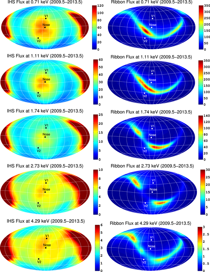
Figure 5. Simulated, time-dependent all-sky maps of flux (in units (cm2 s sr keV)−1) from the IHS (left column) and flux from outside the HP (ribbon flux, right column), linearly averaged over time between 2009.5 and 2013.5 (with 1 yr resolution), for all IBEX-Hi passbands (rows). We also indicate directions toward the nose (259°, 5°), V1 (255°, 35°), and V2 (289°, –32°).
Download figure:
Standard image High-resolution imageBesides the heliotail, there is a relatively strong signature of flux from the nose, similar to previous steady-state, global simulations of H ENA all-sky maps (see, e.g., Gruntman et al. 2001; Heerikhuisen et al. 2007, 2008, 2014; Prested et al. 2008, 2010; Izmodenov et al. 2009), although slightly different than results from a previous time-dependent simulation (Sternal et al. 2008), possibly due to their assumption of a Maxwellian distribution for the IHS plasma. At lower energies, the flux is concentrated near the nose. At higher energies (∼2.73 and 4.29 keV), flux from the nose diminishes and spreads to higher latitudes.
In the right column of Figure 5 we show all-sky maps of flux from outside the HP, i.e., secondary ENAs forming the ribbon. Similar to the solar-inertial frame results from Zirnstein et al. (2013), the ribbon flux at lower energies (∼0.71 and 1.11 keV) is concentrated at low latitudes and then begins spreading to higher latitudes for higher energies (also see McComas et al. 2012b, 2014a). At 2.73 and 4.29 keV, there is a bright emission near the observed knot from IBEX, an indicator of the fast SW at high latitudes. This is an improvement from previous simulations that, although giving ENAs generated in the supersonic SW a speed based on the latitudinal-dependent equations from Sokół et al. (2013) (chosen randomly in time) did not assume that the background SW plasma was time dependent (Zirnstein et al. 2013; Heerikhuisen et al. 2014).
In Figure 6 we show all-sky maps of the total simulated flux (i.e., the sum of the two columns in Figure 5) in the right column, alongside IBEX observations in the left column, from Figure 9 of McComas et al. (2014a). The data and simulation results are shown in the same color scale for each energy. At the lowest energies, the simulated ribbon flux is concentrated near the ecliptic plane, with moderate flux from the nose of the IHS. The simulated flux at this energy appears to match well with observations and is quantitatively similar to the ribbon flux away from the nose. At 0.71 and 1.11 keV, the simulated ribbon peaks in flux since the average slow SW energy is near 1 keV. At higher energies, the simulated ribbon flux diminishes in low latitudes and spreads to higher latitudes as the neutralized SW spreads to higher latitudes, similar to the observations, although somewhat different in absolute intensity. At ∼2.73 and 4.29 keV, simulated flux from the heliotail dominates due to the assumption of constant relative PUI densities, which we use as an approximation. Comparisons to IBEX observations in the left column reveal that this approximation is unrealistic at high energies.
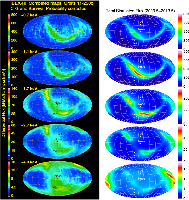
Figure 6. IBEX observations of H ENA flux (left), weight-averaged over the first 5 yr of observations, Compton–Getting and survival probability-corrected, for all IBEX-Hi passbands (from McComas et al. 2014a, Figure 9). On the right we show simulated H ENA flux measurements, linearly averaged over the first 5 yr. All simulation results presented in this paper are computed in the solar-inertial frame, ignoring losses to ENAs within 100 AU from the Sun.
Download figure:
Standard image High-resolution image3.2. Global Changes in Flux since 2009.5
Next we show simulated all-sky maps of the percent change in total flux from 2010.5 to 2013.5, compared to flux simulated in 2009.5, for all IBEX-Hi passbands. This includes primary ENAs from the IHS and secondary ENAs from outside the HP.
3.2.1. Percent Change in Total Flux
Figure 7 shows the percent change in simulated flux for passband 2 (∼0.71 keV). Since 2009.5, the simulated ribbon flux has been decreasing significantly at mid-latitudes. The time in the solar cycle that fueled the 0.71 keV ribbon is approximately 6.5–9 yr earlier, depending on the direction (see Table 2). Therefore, after 2010.5, the ribbon was fueled by primary ENAs created between ∼2001.5 and 2004, which was near the beginning of the decline of the previous solar maximum. During this phase of the solar cycle, the coronal holes are opening up at lower latitudes, increasing in fast ( 2 keV) SW (and thus fast neutral SW), and decreasing in slow (
 2 keV) SW. This causes the decline in ribbon flux at passband 2. Behind the ribbon, the IHS flux also shows variations every year, although partially drowned out by the decrease in ribbon flux. There is a general decrease in flux near the poles, fluctuations near the front and flanks, and little change in the heliotail.
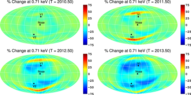
Figure 7. Simulated, time-dependent all-sky maps of the percent change in flux from 2009.5 for IBEX-Hi passband 2 (∼0.71 keV). Regions in yellow to dark red are increases in flux, regions in cyan to dark blue are decreases in flux, and regions in green have little change in flux.
Download figure:
Standard image High-resolution imageAlso notice the bright, nearly horizontal streaks of flux at high (positive and negative) latitudes. These enhancements in flux come from ENAs produced in the IHS where the transition region between fast and slow SW creates two "cusps" of heated, subsonic plasma downstream of the TS that penetrate into the supersonic SW (see Figure 8). As the solar cycle transitions from minimum to maximum, these regions move to higher latitudes and eventually diminish (also see Figures 9–12, as flux from the cusps moves upward over time). While this feature may seem to be artificial due to our assumptions of a "sharp" transition between fast and slow SW, it is known that the fast and slow SW boundary is relatively sharp at solar minimum (see, e.g., McComas et al. 2000); therefore, as the solar cycle transitions from minimum to maximum, this feature may be visible in ENA spectra observed by IBEX, although possibly drowned out by other sources. These features are hardly visible, however, in the time-averaged results shown in Figure 5.
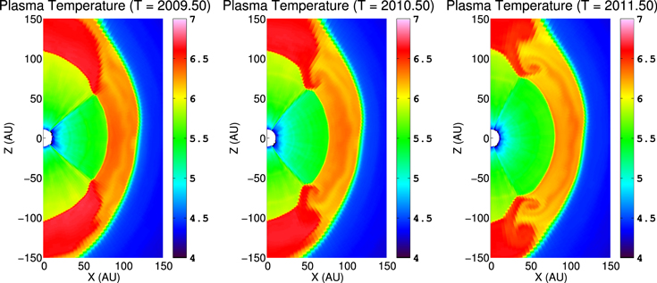
Figure 8. Cross section of plasma temperature (in units log(K)) in the Sun's polar plane, taken 2 yr after solar minimum (2009.5, left), 1 yr later (2010.5, middle), and 2 yr later (2011.5, right). As the SW transitions from solar minimum to maximum, the boundary between fast and slow SW moves to higher latitudes, creating two "cusps" of heated, subsonic plasma that penetrate a considerable distance into the supersonic SW. These cusps also increase the thickness of the IHS, creating the streaks in the IHS flux in Figures 7 and 9–12.
Download figure:
Standard image High-resolution image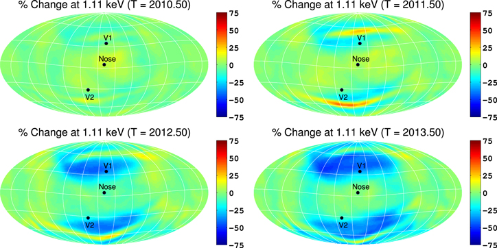
Figure 9. Similar to Figure 7, except for passband 3 (∼1.11 keV).
Download figure:
Standard image High-resolution imageFigure 9 shows the percent change in simulated flux for passband 3 (∼1.11 keV). Similar to 0.71 keV, the ribbon flux decreases at mid- to high latitudes. Also, there is little change in ribbon flux near the ecliptic plane where the average SW speed is relatively constant. At this energy, the percent change in ribbon flux decreases more dramatically at high latitudes compared to 0.71 keV (compare bottom right of Figures 7 and 9). The IHS flux is similar to that at 0.71 keV.
Note that the ribbon shape is barely visible in these maps since the percent change of ribbon flux is nearly uniform, reflecting the nearly uniform decrease in neutralized SW as a function of latitude (also see McComas et al. 2014a). If we were to look at the evolution of absolute flux over time, the largest change would occur in the direction of the ribbon. Also, since the ribbon flux is strongest near the front of the heliosphere, where the HP is closest, we only see a decrease in ribbon flux near the front, and less change from the back.
Figure 10 shows the percent change in simulated flux for passband 4 (∼1.74 keV). At this energy, the ribbon flux begins to increase over time at mid-latitudes and slightly move to higher latitudes. With a total time delay of approximately 6 yr, the source of the ribbon flux measured between 2010.5 and 2013.5 was created between ∼2004.5 and 2007.5. Over this time, the coronal holes were still opening, producing more fast wind, and thus causing an increase in the low-latitude ribbon flux at this energy. Near the poles, there is still a decrease in flux, from both the IHS and OHS (also see Figure 13).
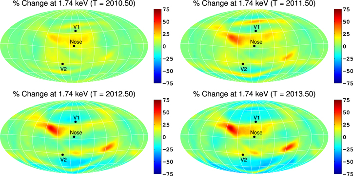
Figure 10. Similar to Figure 7, except for passband 4 (∼1.74 keV).
Download figure:
Standard image High-resolution imageFigure 11 shows the percent change in simulated flux for passband 5 (∼2.73 keV). Similarly to 1.74 keV, the ribbon flux increases as the source of fast neutral SW opens up toward solar minimum. The largest increase in flux occurs near the simulated ribbon knot, which appears in our simulation near (340°, 35°) at this energy and time. Notice that this is lower in latitude than the observed knot, possibly due to our use of simplified SW profiles that determine the outward-propagating ENA speeds. Nevertheless, the knot increases in flux over this period of time, more so than the ribbon flux at negative latitudes. The average fast SW speed is near 2.7 keV; therefore, passband 5 is a good indicator for the evolution of the fast SW at mid- to high latitudes.
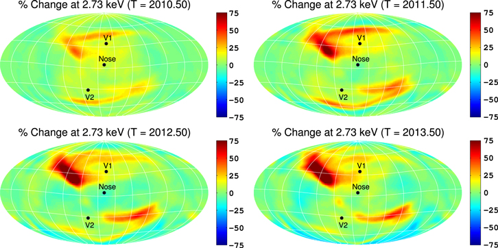
Figure 11. Similar to Figure 7, except for passband 5 (∼2.73 keV).
Download figure:
Standard image High-resolution imageFigure 12 shows the percent change in simulated flux for passband 6 (∼4.29 keV). There is an increase in flux at high latitudes, with the largest increase where the ribbon knot (although faint; see Figure 5) is located near (0°, 45°), where 0° longitude is the fourth longitude line to the left of the nose. At this energy, the delay in time for secondary ENAs from outside the HP is approximately 4.5 yr; therefore, at a measurement time of ∼2013.5, this flux approximately reaches a maximum and will begin to decrease (see Figure 16). The evolution of the IHS flux is also interesting, where we see the two streaks increasing in flux at high positive and negative latitudes, moving to higher latitudes over time. The delay in time for the IHS flux at this energy is within a couple years (depending on the fast or slow SW and the direction of detection); therefore, the source of IHS flux between 2010.5 and 2013.5 is approaching solar maximum, where the transition between fast and slow SW creates two cusps of hot, subsonic plasma downstream of the TS that penetrate into the supersonic SW and move to higher latitudes (see Figure 8). These horizontal streaks are partially visible in Figures 7–12 but are quite distinct at this energy, when the relative flux from the ribbon is not as high.
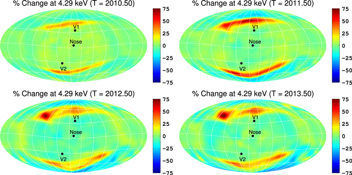
Figure 12. Similar to Figure 7, except for passband 6 (∼4.29 keV).
Download figure:
Standard image High-resolution imageAfter initially increasing in intensity (after 2012.5 and 2013.5 for 4.29 and 2.73 keV, respectively), the knot of emission at these energies also moves to higher latitudes over time while diminishing in intensity, another signature of the evolution of the fast SW toward higher latitudes (i.e., the closing of the coronal holes approaching solar maximum).
Next, we compare the results shown in Figures 7–12 to IBEX data shown in Figure 20 of McComas et al. (2014a). While our results show a continuing decrease in flux for passbands 2 and 3 over a significant portion of the sky (Figures 7 and 9), similar to the data, at higher energies the data also show a global decrease in flux, whereas the simulations show an increase, particularly in the ribbon flux. The simulation results also show that little change occurs in flux from the heliotail, for all energies. While there appears to be a mixture of increases and decreases in flux across the heliotail region in the data (McComas et al. 2014a, Figure 20), on average there is a clear decrease in flux over time (McComas et al. 2014a, Figure 23). These comparisons clearly indicate that the simulations do not reproduce the global evolution of the data, suggesting that the SW dynamic pressure (which is not accurately reproduced in our current simulations) is an important driver of the H ENA flux evolution.
3.2.2. Percent Change in IHS versus Ribbon Flux
Although IBEX measurements are line integrated, meaning separate sources of flux cannot be easily distinguished from each other from a given direction, Schwadron et al. (2011) were able to approximately separate the ribbon and globally distributed flux for the first year of observations (2009), while Schwadron et al. (2014) performed a similar analysis for the first 5 yr of observations, weight-averaged over time. Although there are currently no data on the separated ribbon and globally distributed fluxes as a function of time over the last 4 yr, it is beneficial for this paper to show the percent change in simulated flux for the IHS and OHS (ribbon) separately. While we cannot show the change in flux every year, for every energy and source, in Figure 13 we show the percent change in flux in 2013.5 compared to 2009.5 for the separate sources (IHS flux in the left column, and OHS flux in the right column), at all passbands. In Table 3, we also show percent changes taken from a few directions in Figure 13, to aid the reader.
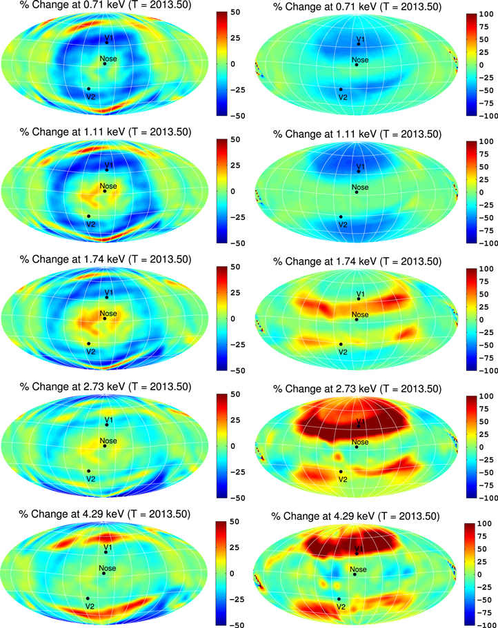
Figure 13. Simulated, time-dependent all-sky maps of the percent change in flux in 2013.5 compared to 2009.5 for all IBEX-Hi passbands (rows), for IHS flux only (left column) and secondary ENA ribbon flux only (right column). Note the different color bar scales for the left and right columns. Also note that the "sharp" fluctuations in flux from the heliotail in the right panels for the ribbon flux are artifacts. These are caused by very low amounts of ribbon flux accumulated from outside the heliotail, near the simulation LISM boundary, which fluctuate as the HP boundary fluctuates. They may also appear "grid-like" due to the angular response, which tends to smooth sharp features.
Download figure:
Standard image High-resolution imageTable 3. Percent Change in Flux in 2013.5, Compared to 2009.5
| Energy (keV) | Nose | S. Flank | N. Pole | Mid-latitude |
|---|---|---|---|---|
| 0.71 | −5/–15 | +7/–19 | −4/–18 | −29/–45 |
| 1.11 | +7/–6 | −6/–8 | −6/–32 | −32/–61 |
| 1.74 | +12/+1 | −10/–1 | −21/–11 | −22/–14 |
| 2.73 | +5/–2 | −6/–16 | −33/+32 | −4/+65 |
| 4.29 | −2/–3 | −4/–36 | −32/+15 | +6/+102 |
Note. The values on the left are for IHS flux, and the values on the right are for ribbon flux. These values are taken from 6° × 6° areas on the all-sky maps in Figure 13, to aid the reader. The nose is averaged around (259°, 5°), the starboard ("S.") flank is averaged around (169°, 0°), the north ("N.") pole is averaged around (–, 90°), and "mid-latitude" is averaged above the nose around (259°, 45°).
Download table as: ASCIITypeset image
The IHS flux both increased and decreased across the maps due to the dynamic SW conditions. At 0.71 keV, the flux fluctuated by a few percent near the nose, decreased by ∼20% approximately 60° away from the nose in the ecliptic plane, decreased in the poles (∼5%–30%), and slightly increased in the tail. The ribbon flux, on the other hand, uniformly decreased at mid-to high latitudes near the front of the heliosphere (∼50%), with less decrease at the poles and ecliptic plane, and little change from the heliotail. The IHS flux at 1.11 keV is similar to 0.71 keV, except with a slightly larger increase at the nose. The ribbon flux decreases uniformly at high latitudes, similar to 0.71 keV, although at a greater rate. The changes in the ribbon flux reflect the source of ∼1 keV, neutralized, supersonic SW that decreases at high latitudes as the last solar cycle approached the recent solar minimum. The changes in IHS flux, however, are more turbulent, reflecting the fluctuations in speed and density of the SW that propagate through the IHS, as well as variations in the thickness of the IHS as a function of space and time.
An interesting feature of the time-dependent SW flow is visible in the IHS flux, particularly for 0.71, 1.11, and 1.74 keV. Although difficult to see in the absolute flux (Figure 5), the variation in flux in Figure 13 shows "rings" of decreased intensity that are symmetric about the nose of the heliosphere. At this time, there is an increase in flux from the nose due to fluctuations in the SW plasma, compared to the flanks and high latitudes. Fluctuations in the IHS plasma, due to either the 11 yr solar cycle or short-term variations, interact the strongest with the nose of the heliosphere, i.e., the closest position from the Sun, and waves propagating through the IHS and reflecting from the HP are the strongest near the nose. This creates higher intensities near the nose and later diminishes and spreads to the flanks and higher latitudes. Also, as the fast–slow SW transition region reaches solar minimum and moves to higher latitudes, it creates these horizontal streaks that appear to "complete" the symmetry.
At 1.74 keV, we see a larger decrease in IHS flux from the poles (∼20%–40%) compared to 1.11 keV, with a similar increase near the nose (∼12%), and a similar decrease in the flanks (∼10%). Again, there is little change in the heliotail; however, there is a slight decrease in flux from the tail near the ecliptic plane (a few percent). At this energy, the ribbon flux has increased at low to mid-latitudes (up to ∼90%), with a slight decrease near the poles (∼10%), and less change near the ecliptic plane. These features are similarly seen at 2.73 keV. The ribbon flux increased dramatically at this energy, which was also evident in Figure 11, with more than double the flux in some areas compared to 2009.5. Changes in the IHS flux at this energy are similar to 1.74 keV, although with a smaller decrease in flux from the flanks.
At 4.29 keV, we can more easily distinguish the high-latitude changes in IHS and OHS (ribbon) flux from Figure 12. The IHS flux is similar to 2.73 keV, although with stronger signatures of the fast–slow SW transition region and less change near the nose. The ribbon flux also more than doubles at high latitudes; however, it is slightly drowned out by the IHS flux in Figure 12.
3.3. Evolution of Flux Spanning a Solar Cycle
In this section we focus more closely on the evolutionary trends of the H ENA flux as a function of energy and direction of detection and predict the trends in the flux relevant for IBEX over the next few years. For the rest of the paper we show simulated spectra spanning at least 11 yr in order to show any evolution with the 11 yr solar cycle.
In Figure 14 we show the directions from which we calculate spectra. For the IHS, we average flux in 6° × 6° areas around three common directions (black contours), including the nose (259°, 5°), V1 (255°, 35°), and the north ecliptic pole (–, 90°). We show spectra from these directions, while only including flux from the IHS, in Figure 15. For the OHS (ribbon), we focus on the north (335°, 35°), middle (282°,  ), and south (225°, –33°) portions of the ribbon, where we average over areas along the ribbon to show the evolution of the ribbon flux as a function of latitude as well as energy, similar to McComas et al. (2014a), although they use larger areas (see their Figures 22 and 23). We show spectra from these directions, while restricting to only secondary ENAs from outside the HP, in Figure 16. Note that McComas et al. (2014a) analyze the evolution of IBEX flux using the spacecraft frame ram maps (corrected for survival probability), instead of flux transformed to the inertial frame, to avoid uncertainties present when transforming from the spacecraft to inertial frame. For simplicity we only simulate flux in the inertial frame of the Sun; however, comparisons of the trend over time are still valid.
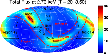
Figure 14. Simulated, time-dependent all-sky map showing directions from which to simulate ribbon spectra. For the IHS flux, shown in Figure 15, we average 6° × 6° areas around the nose (259°, 5°), V1 (255°, 35°), and the north ecliptic pole (–, 90°) directions. For the ribbon flux, shown in Figure 16, we average in larger areas from the north (335°, 35°), middle (282°, –4°), and south (225°, −33°) portions of the ribbon, similar to McComas et al. (2014a). Finally, we show region 1 (ribbon, between the red lines), region 2 (above the northern red line), region 3 (below the southern red line), and region 4 (heliotail, large black contours) similar to McComas et al. (2010, 2012b, 2014a), for which we show the time evolution of the total flux in Figure 19.
Download figure:
Standard image High-resolution image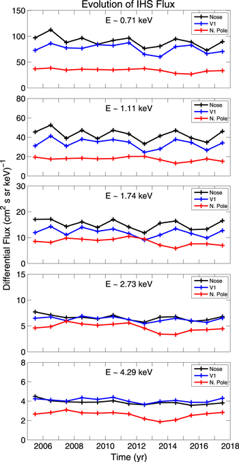
Figure 15. Simulated, time-dependent spectra from the IHS only, from 2005.5 to 2017.5, for all IBEX-Hi passbands. Notice that the IHS flux varies on time scales shorter than the 11 yr solar cycle.
Download figure:
Standard image High-resolution image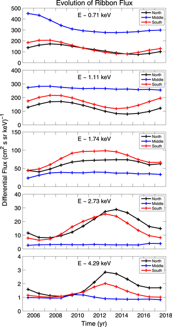
Figure 16. Simulated, time-dependent spectra from outside the HP only (i.e., ribbon flux), from 2005.5 to 2017.5, for all IBEX-Hi passbands. Notice that the ribbon flux varies over time with the 11 yr solar cycle. Note that the small bump in flux in 2009.5 from the middle of the 4.29 keV ribbon is artificial, due to statistical fluctuations at high energies when computing the 6D H distribution.
Download figure:
Standard image High-resolution imageIn Figure 14 we also show four global regions where we compare the total flux to IBEX observations, which cannot easily distinguish between flux from different sources along an LOS (however, see Schwadron et al. 2011, for separated ribbon results). Region 1 (between the red lines) encompasses the ribbon, region 2 (above the northern red line) encompasses all flux above the ribbon, including the north pole, region 3 (below the southern red line) encompasses all flux below the ribbon, including the south pole, and region 4 (black contours) encompasses most of the heliotail. Similar to McComas et al. (2014a), any flux included in region 4 (the heliotail) is excluded from other regions. We compare the fraction change in simulated flux from these four regions in Figure 19 to IBEX data from similar regions as defined in McComas et al. (2014a).
3.3.1. Short-term Fluctuations in the IHS Flux
In Figure 15 we show simulated, time-dependent spectra of IHS flux only, between 2005.5 and 2017.5, for all IBEX-Hi passbands. We take spectra from three common directions, i.e., the nose, V1, and north ecliptic pole. It is immediately evident that the IHS flux changes on timescales shorter than the 11 yr solar cycle, dominated by fluctuations in the background SW plasma, e.g., variations in the thickness of the IHS as a function of space and time. There is a consistent oscillation in flux at all energies, with a period between ∼2 and 6 yr that depends on the direction. At high energies, the oscillations in flux from the nose and V1 directions become less noticeable; however, they are stronger from the north ecliptic pole.
Reisenfeld et al. (2012) analyzed the time dependence of IBEX-Hi measurements from the north and south ecliptic poles over the first 2 yr of IBEX operation (2009–2011), showing an energy-dependent drop in flux over time. They showed that little change occurred at 0.71 keV, the most significant drop occurred at ∼1.1 keV, and variations in flux occurred with periods  6 months. Unfortunately, our simulations cannot reproduce variations on such short timescales. Nonetheless, it appears that our simulations indicate a small increase in flux from the north ecliptic pole direction for some energies, for the first 2 yr (2009.5–2011.5), in contrast to the observations. This is likely an indication that our simulations still do not accurately capture the decrease in SW ram pressure during the recent solar minimum. However, careful comparisons with IBEX-Hi data from the polar regions are left for future studies.
The phase of the oscillations in flux slightly depends on energy, but more obviously on the direction of detection. For instance, flux from the nose and V1 directions appears nearly in phase for all energies, although the V1 spectra are slightly behind. Flux at all energies, at low latitudes, oscillates with a period of approximately 2–4 yr, whereas at higher latitudes (i.e., north ecliptic pole), the oscillation period appears longer, although difficult to determine. These results reflect the differences in fluctuations in the background plasma as a function of latitude. Contrary to the observations, there does not appear to be a significant decrease in flux from the IHS from these directions, except for the drop between ∼2010.5 and 2013.5.
3.3.2. Long-term Evolution of the Ribbon Flux
In Figure 16 we show simulated, time-dependent spectra of ribbon flux only, between 2005.5 and 2017.5, for all IBEX-Hi passbands. We take spectra from the north, middle, and south portions of the ribbon to study the evolution of the ribbon flux as a function of latitude as well as energy, similar to McComas et al. (2014a). The ribbon flux shows considerable change over time, with little evidence of small-scale fluctuations due to the turbulent solar cycle. This is likely due to the weighted contribution of PUIs averaged over 3 yr (a realistic process), as well as the long integration length through the OHS.
Our results show that the secondary ENA ribbon flux evolves with the solar cycle, with a period out of phase by the times of ENA propagation and PUI-to-ENA charge exchange. This, of course, depends on the direction of detection and the energy of the ENAs. For 0.71 keV, flux from all three directions decreases in intensity from 2009.5 until ∼2013–2015.5. The delay in time between creation of parent ENAs and measurement of secondary ENAs is approximately 6.5–9 yr; therefore, the source of parent ENAs is during the fall of the last solar maximum, which began around ∼2001.5. There is a full recovery of flux at 0.71 keV after ∼2013–2015.5, depending on the direction of detection.
3.3.3. Asymmetries in the Ribbon Flux Evolution
As pointed out by McComas et al. (2014a), the distance to the HP will play a large role in the delay time between measurements from the north and south portions of the secondary ENA ribbon, where we should expect a recovery of flux from the south before the north. For example, toward the southern portion of our simulated ribbon, the HP is relatively close to the Sun (∼140 AU; see Figure 17) due to the interstellar magnetic pressure on the HP. However, we note that the OHS plasma and neutral densities also play a significant role. The densities are larger near the southern portion of the ribbon than the north since it is closer to the nose of the heliosphere, where the plasma experiences the most compression. These larger densities effectively reduce the mean free path of ENAs in the OHS (due to a large plasma density) and reduce the PUI-to-ENA charge-exchange time (due to a large neutral density). Therefore, the source of ENAs from this region is relatively close (i.e., short distance to the HP and short distance of propagation through the OHS), and thus they are detected at an earlier time, with a recovery in flux occurring in 2014. In the middle of the ribbon, the HP is slightly closer (∼130 AU), and the plasma and neutral densities are slightly larger (see Figure 17). While the differences in these parameters compared to the south will complicate the total time delay (e.g., larger plasma density will reduce the ENA mean free path), overall the phase of the flux from the middle of the ribbon is similar to the south, although recovering slightly sooner. Flux from the northern region originates the farthest away (∼170 AU), from a region of the OHS with significantly lower plasma and neutral densities (thus larger ENA mean free path and PUI-to-ENA charge-exchange time). These changes overall cause the flux to be delayed by ∼2 yr compared to the south (see Table 2 for approximate time delays), such that the flux continues to decrease until ∼2015.5 and then recovers. These trends are similarly seen in recent IBEX observations, where flux from the southern part of the IBEX ribbon appears to be leveling off in 2013, while flux from the north continues to decrease (see McComas et al. 2014a, Figure 28).
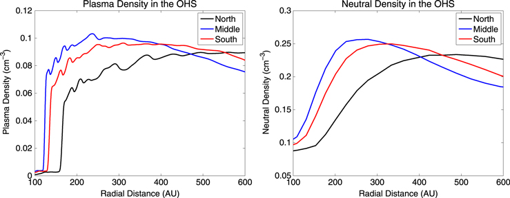
Figure 17. Plasma (left) and neutral (right) densities along radial lines through the OHS, toward the north (335°, 35°), middle (282°, –4°), and south (225°, –33°) regions of the ribbon, taken in 2009.5. Notice the large densities toward the middle and south directions, due to the interstellar flow and magnetic pressure on the HP. This reduces the ENA mean free path and PUI charge-exchange delay time compared to the north. The fluctuations in plasma density are caused by pressure waves propagating from the inner heliosphere (mainly generated by the 11 yr solar cycle) out to the HP and through the OHS. The bulk neutral density is, however, weakly coupled to the plasma, and these oscillations do not appear in the neutral density profiles.
Download figure:
Standard image High-resolution imageFlux simulated at 1.11 keV produces a similar trend to passband 2, with the latest recovery occurring in the north after 2015, and the earliest recovery after 2013.5 in the south. Again these are largely due to the differences in the distances to the ENA source, as well as the difference in plasma and neutral densities in the OHS. The recovery times are slightly earlier at this energy since the ENAs are faster and thus are detected sooner than at 0.71 keV, particularly in the north. Flux from the middle region appears to be the most stable, with little evidence of the 11 yr solar cycle. This is likely due to the nearly constant source of slow SW near 1 keV in our simulations (although fluctuating about the mean; see Figure 2); and thus slow primary ENAs that fuel the secondary ENA flux at this energy.
It is important to note that higher-energy parent ENAs will travel farther through the OHS before charge exchange occurs, compared to lower-energy ENAs, due to the energy-dependent, charge-exchange cross section (e.g., Möbius et al. 2013). However, even though the mean free path increases with energy, the propagation and charge-exchange times decrease. Also, near the front of the heliosphere the plasma and neutral densities typically increase farther away from the HP, up to the H wall/bow wave (see Figure 17; also see Zank et al. 2013; Heerikhuisen et al. 2014). This, in effect, reduces the distance that high-energy parent ENAs can travel through the OHS before charge exchange. While the time-delay estimates shown in Table 2 may oversimplify the effective mean free path for H ENAs through the OHS, our simulation results suggest that higher-energy secondary ENAs from the ribbon are detected slightly sooner than lower-energy secondary ENAs.
3.3.4. Predicted Increase in High-energy Ribbon Flux
At 1.74 keV, there is a significant change in the evolution of the simulated ribbon flux. At this energy, as expected we are detecting fewer secondary ENAs at lower latitudes and detecting more at higher latitudes. Again, this is due to the existence of faster SW at higher latitudes. The delay in time between parent ENA creation and secondary ENA detection is approximately 5–7 yr; therefore, the fuel for these secondary ENAs was created at a time in the solar cycle beginning in ∼2003.5, during the decline of the last solar maximum. There is no longer a steady decline in flux, like at 0.71 and 1.11 keV, but rather a slight increase, most noticeable in the north and south, and an eventual decline after ∼2013–2014.5. In the middle of the ribbon, there is less flux and only slight variability. While the evolution of flux from low latitudes appears to show slight variation with the short-term solar cycle, flux from higher latitudes is more obviously driven by the transition between fast and slow SW, i.e., the 11 yr solar cycle.
To illustrate this, in Figure 18 we show cross sections of the plasma speed in the Sun's polar plane over the course of the solar cycle. Near solar minimum, the fast SW reaches down to lower latitudes near ±35°. At this time, interstellar H atoms at mid- to high latitudes have a higher probability to survive charge exchange in the slow SW, and instead charge exchange in the fast SW, creating a fast primary ENA. Near the ecliptic plane, however, most interstellar H atoms will, on average, charge exchange in the slow SW (although the SW speed is highly variable at low latitudes; see, e.g., Sokół et al. 2013, which is not reproduced in our simulations). As the solar cycle transitions from minimum to maximum, the slow SW spreads to higher latitudes, reducing the probability of creating fast primary ENAs and thus fast secondary ENAs. This, in effect, creates a maximum in the high-energy flux when the source of secondary ENAs was created near solar minimum, and a minimum in the high-energy flux when the source of secondary ENAs was created near solar maximum, and vice versa for the low-energy flux (also see McComas et al. 2012b, 2014a, for a similar discussion). These maxima and minima are not in phase with the solar cycle, nor with each other, but are delayed by the propagation and charge-exchange delay times as a function of energy and direction. We stress, however, that this process is likely more complicated than we can currently simulate, especially considering our simplified model of the SW.
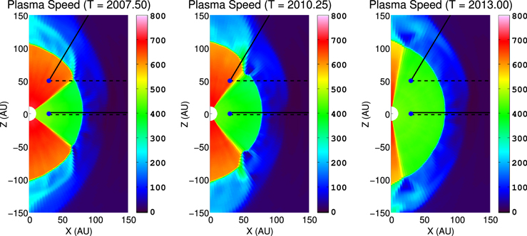
Figure 18. Cross section of plasma speed (in units km s−1) in the Sun's polar plane, taken during solar minimum (left, 2007.5), solar maximum (right, 2013), and halfway between (middle, 2010.25). Shown are trajectories of interstellar H (solid black lines) and primary H ENA (dashed black lines) atoms that traverse the inner heliosphere. During solar minimum, interstellar H atoms have a higher probability to survive charge exchange until they reach the fast SW region, creating more high-energy ENAs. At solar maximum, this probability is decreased.
Download figure:
Standard image High-resolution imageReturning to the flux profiles in Figure 16, at higher energies, we see a global change in the simulated ribbon evolution, where we are now detecting high-energy ENAs that were created in the fast SW. At 2.73 keV, there is even less flux at lower latitudes, with little visible variation over time. At this energy, the peak in the flux in the north and south occurs sooner than the recovery of flux at 0.71 and 1.11 keV. The delay in time between parent ENA creation and secondary ENA detection is approximately 5 yr; therefore, the peak in flux corresponds to the last solar minimum, which began in ∼2007.5. The peak in flux in the south occurs first in 2012.5 and later in the north in ∼2013.5. This energy is particularly important since it is approximately equal to the average energy of the fast SW, where v = 723 km s−1. Therefore, our results show the largest relative change in flux compared to all other passbands, where the transition from slow to fast SW, and thus slow to fast parent ENAs, is reflected strongly in the ribbon flux.
At 4.29 keV, the ribbon flux from all directions is considerably diminished because we are detecting ENAs at speeds near 900 km s−1, which is higher than the average fast SW speed. However, the IBEX-Hi energy response has an FWHM of ∼0.6–0.7E for passbands 2–6, where E is the nominal energy for each passband (Funsten et al. 2009a; McComas et al. 2012b). This allows IBEX-Hi to detect ENAs with energies lower and higher than the nominal energy (in this case 4.29 keV). The energy response functions are applied in our simulations.
While there is little change in the middle of the ribbon at 4.29 keV, there is still an increase in flux from the southern and northern regions. The delay in time between parent ENA creation and secondary ENA detection is approximately 4.5 yr, where the peaks again approximately correspond to the last solar minimum. Surprisingly, the peaks in flux from the north and south appear at nearly the same time in 2012.5. However, this is due to our choice of the northern direction from which to show simulated flux (see Figure 14). As the solar cycle approaches maximum, the majority of fast neutralized SW only exists at higher and higher latitudes, causing the simulated flux from the ribbon at high energies (at a sufficient time later) to appear at higher and higher latitudes. The direction to  reaches relatively high latitudes near the north region (up to +60° latitude), but not as "high" in the south region (down to –45°). Therefore, flux from the south region will peak and quickly diminish as the source of fast neutralized SW moves to higher (negative) latitudes, resulting in the flux from the south abruptly decreasing after 2012.5. Flux from the north, however, only gradually decreases after 2012.5 since the high-energy flux from the north is still visible at 1 AU up through +60° latitude. However, our chosen "north" direction is lower than this limit, and the flux from the north actually peaks at higher latitudes approximately a year later in 2013.5.
It is important to reiterate the implications of our assumptions for the SW boundary conditions beyond 2011.5 on our simulated ribbon results. At 1.74 keV, the delay in time between parent ENA creation and secondary ENA detection is ∼6 yr (assuming a distance through the OHS within which the majority of ENA flux has been accumulated, beyond which the time is even further in the past). Therefore, a detection of ENAs at this energy in 2017.5 corresponds to a solar cycle time of ∼2011.5, which is within the range of data from Sokół et al. (2013). For 2.73 keV, the delay is ∼5 yr; thus, simulations of measurements made after 2016.5 can only be approximated by predicting the SW boundary conditions. Therefore, a simulation of flux for passbands 5 and 6 beyond 2016.5 is dependent on assumptions we make for the SW, while flux from passbands 2–4 can be reasonably simulated approximately 6 yr into the future. More recent measurements of the SW in the ecliptic plane could be extracted (see, e.g., McComas et al. 2013); however, we used the data from Sokół et al. (2013) to provide SW speeds and densities as a function of latitude to compute H ENA speeds created in the supersonic SW, which will better represent the energy distribution of the secondary H ENA flux. The IHS flux depends more strongly on SW boundary conditions closer to the time of measurement and therefore cannot be accurately predicted more than a few years ahead of the data, at least for IBEX-Hi energies.
3.4. Comparisons to the Evolution of IBEX Data
Finally, we want to show the global changes in flux over time, similar to the analysis of McComas et al. (2012b, 2014a), and compare to observation. In Figure 19 we show the fraction of simulated, time-dependent spectra of the total flux (IHS + OHS), compared to 2009.5, from regions 1–4 as defined in Figure 14. In the top left panel we show the evolution of the total flux averaged over region 1 (ribbon), divided by the flux simulated in 2009.5. Since most of the simulated flux from this region is from secondary ENAs from outside the HP, the lowest energies decrease over time since 2009.5 and slightly recover after ∼2013.5, with a faster recovery after 2016.5 (the total flux evolution is slightly different from the separated ribbon flux evolution; see Figure 16). At higher energies, unlike in the observations, the simulated flux increases over time since 2009.5, peaks between ∼2011.5 and 2013.5, and decreases later on. This initial increase at high energies is not seen in the IBEX data, which show a nearly uniform drop in flux at most energies. While there is little change at 4.29 keV in the simulation, significant variation occurs at 2.73 keV. As stated previously, this energy is equal to the average energy of the fast SW and therefore should be most affected by our approximation of the transition between fast and slow SW.
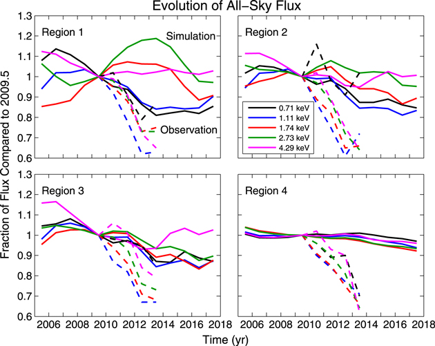
Figure 19. Fraction of simulated (solid lines) and observed (dashed lines), time-dependent flux compared to that simulated/observed in 2009.5, for region 1 (ribbon), region 2 (nose, north pole), region 3 (south pole), and region 4 (heliotail), as defined in Figure 14 (red and black contours) for the simulations and Figure 23 from McComas et al. (2014a) for the observations. Notice that most of the variation in the simulated flux occurs near the ribbon, although the decrease in the observed flux from all regions is significantly stronger than in the simulation results.
Download figure:
Standard image High-resolution imageIn the top right panel of Figure 19 we show the evolution of the fraction of total flux from region 2 (nose, north pole). Except for 1.74 and 2.73 keV, there is a general decrease in simulated flux since 2009.5, until approximately 2014. After 2011.5, flux at 1.74 keV continues to drop until ∼2016.5, and flux at 4.29 keV recovers by ∼2013.5. The flux from this region is a mixture of secondary ENAs from outside the HP (although less intense compared to region 1) and primary ENAs from the IHS. Since the ribbon flux dominates at 0.71, 1.11, and 2.73 keV, these simulated spectra experience the most change. However, similar to the flux from region 1, the decrease in the observed flux is much stronger than in our simulations. We see a similar behavior in the bottom left panel, which shows the evolution of the fraction of total flux from region 3 (south pole).
In the bottom right panel, we show the evolution of the fraction of total flux from region 4 (heliotail). Although we may not accurately simulate the absolute flux from PUIs in the heliotail, as described in Section 3.1, we do not expect a significant difference in the relative change in flux over time, between our simulation and a more accurate solution for PUIs. As one can see, from this region there is the least difference in the trend over time of the simulated flux between each energy. For most energies, there is only a slight change in flux, small compared to the large decrease in the observed flux.
In Figure 20 we compare the simulation results with the data from the north and south ribbon regions defined in Figure 27 of McComas et al. (2014a), with the only difference being our definitions of the ribbon and heliotail contours (compare Figure 14 in this paper to Figure 22 in McComas et al. 2014a). McComas et al. reported that a recovery in flux may be occurring in the southern portion of the ribbon in the latest data, whereas flux from the north continues to decline in intensity. In the north, the simulation results at low energies appear to decline along with the data, with the beginning of a recovery after 2013.5. At higher energies, again we see a significant deviation in the evolution of the results compared to the data. In the south, it is more difficult to determine a point at which a recovery occurs. Unlike in Figure 16, which showed simulation results from the small regions defined in Figure 14 (and only accounting for ENAs from the OHS), showing times of clear recovery in the south before the north, the results shown in Figure 20 are averaged over much larger regions (and accounting for ENAs from the IHS and OHS), smearing out this effect in our simulation results.

Figure 20. Fraction of simulated (solid lines) and observed (dashed lines), time-dependent flux compared to that simulated/observed in 2009.5, for the north (top) and south (bottom) ribbon regions defined in Figure 27 from McComas et al. (2014a). The simulated flux is averaged from the same latitude boundaries defined by McComas et al., although the simulated ribbon region is slightly different than the observed ribbon (i.e., the region inside the red contours; see Figure 14 in this paper).
Download figure:
Standard image High-resolution image
As is evident in Figures 16, 19, and 20, our results at higher energies ( keV) do not appear to agree with the initial trend of IBEX observations. Our results deviate the most in the 2.73 keV ribbon flux, which experiences the most variation over time. This is possibly due to our simplified assumptions of the uniform fast SW speeds and densities, or there may be a missing physical mechanism occurring at high energies for PUIs in the OHS that is not included in our model.
Also, our simulations are not able to reproduce the large decrease in solar flux and ram pressure during the recent, extended, solar minimum (see Figure 29 from McComas et al. 2014a), which likely explains the large discrepancy between the magnitude of variations in our simulations compared to the observations (compare the results of this paper to Figures 20, 23, and 28 in McComas et al. 2014a). Comparisons between our results and the observations strongly suggest that the SW dynamic pressure is an important driver of the evolution of the IBEX flux, perhaps more important than the 11 yr solar cycle. However, our results appear to qualitatively agree with IBEX observations in some respect, where both observation and simulation see signs of recovery in the flux after ∼2013.5 in the southern part of the ribbon, but a continued decrease in flux from the north (see Figure 16).
4. CONCLUSION
IBEX observations have shown that the global ENA flux is changing with time, with an overall decrease in intensity since initial observations in 2009 (McComas et al. 2010) and apparent signs of recovery in the latest observations (McComas et al. 2014a). With a data set spanning 5 yr, these observations are allowing us to indirectly view the time-dependent heliosphere. With sophisticated modeling, we hope to offer insight into these observations and predict measurements for the coming years. In particular, the strongest ENA signal in the sky, the ribbon, shows significant signs of evolution in the observational data. An important goal to understanding these observations is determining the origin of the IBEX ribbon. Therefore, in this paper we (1) demonstrate how the secondary ENA ribbon evolves over time (based on our time-dependent model assumptions) and (2) show that, while the secondary ENA mechanism reproduces some evolutionary characteristics that are qualitatively similar to what IBEX has observed, in reality the time-dependent ribbon is more complicated than previously thought and cannot be accurately modeled using the somewhat idealized assumptions applied in our simulation.
We first obtained simulated, heliospheric results using our 3D, time-dependent MHD-plasma/kinetic-neutral simulation of the SW–LISM interaction, and we used these results as a time-dependent "background" heliosphere for our post-process H ENA flux simulations. By propagating along H ENA trajectories backward in time from the time of measurement to the time of ENA (or parent PUI, for the ribbon) creation, we are able to interpolate plasma and neutral results in space and time and simulate a time-dependent IBEX ribbon, as well as IHS flux, as described in Section 2.
For simplicity, in our MHD/kinetic simulation we assumed that the fast and slow SW had uniform values over their respective regions, although the speeds and densities, as well as the transition between fast and slow SW, varied as a function of time. This assumption affects the probability of charge exchange between the plasma and neutrals, which is a function of the local plasma and neutral properties. However, in our MHD/kinetic simulation, ENAs born in the supersonic SW were given speeds derived from the latitude and time-dependent equations from Sokół et al. (2013), rather than gaining speeds directly from the local plasma (in fact, the SW speed and density boundary conditions for the MHD/kinetic simulation were also taken from Sokół et al. 2013). While this improved the energy characteristics of the parent ENA (and thus secondary ENA) distribution, the rate of charge exchange still depends on the local plasma conditions. Implementing the latitude-dependent equations for speed and density provided by Sokół et al. (2013) and longer-term variations in the SW output (McComas et al. 2014a) directly in the MHD/kinetic simulation is a necessary step to take in future work.
In Section 3 we showed the results of our time-dependent simulations, presenting all-sky maps of the IHS and OHS (ribbon) flux, the evolution of the global maps from 2009.5 to 2013.5, as well as simulated spectra over an 11 yr period. As is evident in our results in Section 3.1, the ribbon flux experiences the most significant variation over time with the 11 yr solar cycle. There is a general decrease in flux over the entire ribbon at 0.71 and 1.11 keV since 2009.5 (Figures 7 and 9), where the ribbon flux decreases at mid- to high latitudes. At higher energies, the ribbon flux actually increases over time, at least until ∼2013, which is due to the production of more fast SW at lower latitudes. The IHS flux showed less signs of periodicity with the 11 yr solar cycle, but rather showed short-term fluctuations due to the turbulent background IHS plasma. Interesting features of the transition between fast and slow SW were visible in the IHS flux (i.e., cusps), which may be useful signatures to look for in the IBEX data, assuming they are not overpowered by other sources.
In Section 3.3 we showed the evolution of ENA flux in more detail, looking at various directions in the sky and showing the evolution of flux from 2005.5 to 2017.5. The IHS flux is obviously dependent on the local, turbulent IHS plasma conditions, fluctuating with periods that depend on the local wave period in the IHS, which is likely different for the slow and fast SW plasma in the IHS. Our results show the most variability in the IHS flux from lower latitudes, at lower energies, with less variability from higher latitudes, at higher energies. Unlike the ribbon flux, there is little evidence of an 11 yr period in the IHS flux, although we have yet to analyze this in detail.
The ribbon flux not only changes over time but appears periodic with the solar cycle, out of phase by an amount of time that depends on the energy and direction of detection. For lower energies, the ribbon flux recovers sooner in the south and later in the north (see Figure 16), which appears to be consistent with the observations. As explained by McComas et al. (2014a), as a characteristic of the secondary ENA mechanism, this is likely due to the larger distance to the HP in the north than the south, with an increased interstellar magnetic pressure in the south, and the fact that the southern ribbon region is closer to the front (compressed) side of the heliosphere, while the northern ribbon region is at higher latitudes, nearer to the flanks. We stress that the OHS plasma and neutral densities are also larger in the southern portion of the ribbon (see Figure 17), reducing the mean free path of parent ENAs and the PUI charge-exchange time. These differences may be an important indicator to look for in IBEX observations. If, as the data suggest, the recovery of the observed ribbon flux at these energies occurs sooner in the south than the north, not only do we have more evidence that the secondary ENA mechanism is responsible for creating the ribbon, but this can help constrain the distance to the HP in different directions, as well as the OHS plasma properties. This may also help constrain the strength and direction of the interstellar magnetic field necessary to distort the time-dependent heliosphere in such a way as to reproduce this asymmetry in measurement time.
For some high energies and directions, our simulations predict the ribbon flux increases over time from 2009.5 until ∼2012.5–2014. These results do not appear to agree with IBEX observations; however, it is likely due to our simplified assumptions for the SW boundary conditions, defining the slow and fast SW as uniform, but separate, regions, or high-energy PUI dynamics that are not taken into account in our simulation. Nevertheless, these results may still provide useful insights into IBEX data, while keeping in mind the assumptions used in the MHD/kinetic simulation.
In Figure 17 we showed the plasma and neutral densities in the OHS, where pressure waves in the OHS plasma propagate away from the HP at the local magnetosonic speed, approximately 8 AU yr−1 = 38 km s−1, eventually slowing and dissipating farther away from the HP. These waves are largely generated by the 11 yr solar cycle that propagates through the IHS and cross the HP with a period near 2–4 yr (see, e.g., Pogorelov et al. 2009a). However, there is little evidence of these OHS plasma oscillations in the ribbon flux simulations. This is partly due to the weighted-averaging of PUIs when computing the secondary ENA flux (with a mean charge-exchange time approximately equal to the period of these waves), as well as the long LOS integration through the OHS (the H ENA flux propagates at speeds much larger than the wave speed), which will tend to average out fluctuations in the background plasma. Also, since we should expect any fluctuations in the ribbon flux to vary with ENA energy, the IBEX energy responses, with FWHM ∼0.6–0.7E, will smooth out these features.
There appears to be little variability in the ribbon flux due to the shorter-scale plasma fluctuations. If there are fluctuations in the ribbon, they would most likely be visible near the ecliptic plane, where there is a nearly constant source of slow neutralized SW, and thus will not be largely affected by the transition between fast and slow SW (see Figure 16, "middle"). It would be unlikely that these short scale fluctuations are caused by fluctuations in the background OHS plasma, but rather by variations in the outward-propagating, parent ENA distribution, induced by variations in the supersonic SW. However, in reality the fluctuations in the observed SW are not as smooth, nor with as long periods, as that used in our simulations, and are beyond the scope of this paper to analyze.
While we made improvements to the time-dependent heliosphere from Pogorelov et al. (2009a) by implementing the time-dependent SW boundary conditions from Sokół et al. (2013), the distance to the HP in our simulations is still overestimated (∼140 AU in the V1 direction), based on the recent crossing of the HP by V1 (Gurnett et al. 2013). We also do not accurately simulate Rayleigh–Taylor instabilities at the HP, which may explain the observations (Borovikov & Pogorelov 2014). However, if the distance to the HP is shorter by ∼20 AU as the V1 data suggest, the total propagation times for ENAs (parent ENAs going out and secondary ENAs coming in) will decrease by ∼0.5 and 0.2 yr for 0.71 and 4.29 keV ENAs, respectively. Therefore, our results are generally valid even for a thinner heliosheath, only overestimated at most by half a year.
Kucharek et al. (2013) suggested that the fast temporal changes observed in the IBEX ribbon flux may be explained by a different mechanism, a ribbon created near the TS with a small line-integration length (∼1–2 AU). Using simple pressure balance arguments, the authors suggested that a significant amount of flux may be produced by ion ring distributions at the TS. Whether the true PUI and wave-particle dynamics at the TS would allow a sufficient amount of flux from such a small integration length is still unknown, although this may be pursued by Kucharek et al. (2013) in the future. While the results of our simulations do not show significant fast temporal changes in the ribbon flux, the large-scale trends are reproduced reasonably well, at least at low energies. It is important to note that the SW boundary conditions we used are derived from yearly averages, which we then interpolate to a 3-month scale. This will not be able to reproduce short timescale fluctuations actually observed in the SW, and thus not in the ribbon flux. It is also difficult to determine, when looking in the direction of the observed ribbon flux, whether the fast temporal changes are indeed from the ribbon source or from an IHS source along the same integration path. While our simulations suggest that most short-scale fluctuations are visible in the IHS flux, more sophisticated modeling of the time-dependent SW will hopefully offer additional insight into these effects.
It has recently been shown that the center of the IBEX ribbon at high energies is different than at low energies (Funsten et al. 2013). Funsten et al. proposed that this may be a time-dependent effect, where the center of the ribbon may change over time, but changes in the observed ribbon center at low energies are delayed due to their slower speeds. As a next step we will study the time dependence of the center of our simulated ribbon, as a function of energy, and hopefully offer clues that will help determine the cause of these effects.
Finally, we reiterate that the biggest discrepancy between the observations and simulation results is the large decrease in flux at all energies in the data over the past 5 yr, which is not seen in the simulation results. At this time we can only postulate several explanations for this discrepancy: (1) our idealized SW boundary conditions for the fast and slow SW regions do not accurately represent the 11 yr solar cycle; (2) our simulations do not reproduce the significant drop in solar flux and dynamic pressure as seen in observations of the SW; (3) our simulations do not incorporate any evolution in the LISM structure, such as a significant drop in interstellar H density. While any changes in the LISM would likely act over timescales much larger than 5 yr, in future work we can introduce time-dependent LISM boundary conditions. However, the most likely explanation is the lack of realistic boundary conditions for the SW dynamic pressure, which will be improved in future work.
E.Z. acknowledges support from NESSF grant NNX11AP91H. J.H. and N.P. acknowledge support in part from NASA grants NNX11AB48G, NNX12AH44G, NNX12AB30G, NNX13AF99G, NNX14AF43G, NNX14AP24G, and NNX14AJ53G, and DOE grant DE-SC00008334. This work was made possible in part by a grant of high-performance computing resources and technical support from the Alabama Supercomputer Authority. This work was also carried out as part of the IBEX mission, which is part of NASA's Explorer Program.
: APPENDIX
We simulate the 3D, time-dependent SW–LISM interaction using an MHD description of a single-fluid plasma, coupled to a kinetic description of neutral H atoms (e.g., Heerikhuisen et al. 2006a, 2006b, 2013; Pogorelov et al. 2008b, 2009a). We solve the ideal MHD conservation equations of mass, momentum, energy, and magnetic flux, given by, respectively,
where ρ is mass density,  is plasma velocity, e is total energy density,
  is the magnetic field vector,
  is total pressure (assumed to be isotropic), and
  is the 3 × 3 identity matrix. System (A1) is written in the symmetrizable, Galilean-invariant form proposed by Godunov (1972), which proved to be useful for the purpose of eliminating spurious magnetic charge (Pogorelov & Matsuda 1998; Linde et al. 1998; Powell et al. 1999). The MHD equations are solved using a total variation diminishing Courant–Isaacson–Rees scheme with second-order accuracy in space and time (Kulikovskii et al. 2001). On the right-hand side of Equation (A1) are momentum (
 ) and energy (
 ) source terms due to charge exchange and photoionization of neutral H atoms, as well as a mass source term (
 ) due to photoionization of neutral H. The coordinate system of the simulation is constructed such that the z-axis is aligned with the solar rotation axis, the +x-axis lies in the plane containing the z-axis and the LISM inflow direction ((259°, 5°) in ecliptic J2000 coordinates), and the y-axis completes the right-hand coordinate system.
The neutral H atoms are governed by the Boltzmann transport equation, given by

where fH is the neutral H distribution,  is the neutral H velocity,
  is an external force (i.e., gravity and radiation pressure, which are assumed to be balanced), mH is the mass of H, and P and L are the production and loss source terms for neutral H, respectively, given by

where fp is the proton distribution, η is the production rate for neutral H due to charge exchange, and β is the loss rate due to charge exchange and photoionization. Equation (A2) is solved using a Monte Carlo approach (e.g., Heerikhuisen et al. 2006a, 2006b), where a sufficiently large number of particles (∼109) are used in the simulation. Unlike in steady-state calculations that can run the kinetic-neutral code for arbitrarily long times to collect enough statistics (e.g., Heerikhuisen et al. 2006a, 2006b), in a time-dependent simulation the kinetic-neutral code cannot be run longer than the timescales to be resolved. In this work, the kinetic-neutral code is run on a scale of 3 months in order to resolve the 11 yr solar cycle (Heerikhuisen et al. 2013). However, the number of charge-exchange events in the computational grid is limited by this short amount of time. Therefore, we improve the statistics of charge exchange by (1) introducing a larger number of particles into the simulation and (2) repeating each step of the kinetic-neutral code multiple times, each with slightly perturbed initial positions, and averaging over these "multiple realizations" (see Heerikhuisen et al. 2013).
The mass, momentum, and energy source terms computed by the kinetic-neutral code are given by, respectively,
where mi is the particle's simulation weight (mass of H times the computational weight), Ni and  are the number of H atoms before and after photoionization,
  and
and  are the velocities of H atoms before and after charge exchange (photoionization), and Nph and
  are the number of H atoms that photoionize and charge exchange (photoionize), respectively, during a time
  , in volume
  . After running the kinetic neutral code for
  yr, collecting a sufficient number of events (Nph,
  ) and "multiple realizations," the MHD-plasma code is then run with these source terms (Equation (A1)). This process is repeated until the required time evolution is simulated (see the simulation flowchart in Figure 1).