


Abstract
The remanent magnetization of solar system bodies reflects their accretion mechanism, the space environment in which they formed, and their subsequent geological evolution. In particular, it has been suggested that some primitive bodies may have formed large regions of coherent remanent magnetization as a consequence of their accretion in a background magnetic field. Measurements acquired by the Rosetta Magnetometer and Plasma Monitor have shown that comet 67P/Churyumov–Gerasimenko (67P) has a surface magnetic field of less than 0.9 nT. To constrain the spatial scale and intensity of remanent magnetization in 67P, we modeled its magnetic field assuming various characteristic spatial scales of uniform magnetization. We find that for regions of coherent magnetization with ≥10 cm radius, the specific magnetic moment is ≲5 × 10⁻⁶  . If 67P formed during the lifetime of the solar nebula and has not undergone significant subsequent collisional or aqueous alteration, this very low specific magnetization is inconsistent with its formation from the gentle gravitational collapse of a cloud of millimeter-sized pebbles in a background magnetic field ≳3 μT. Given the evidence from other Rosetta instruments that 67P formed by pebble-pile processes, this would indicate that the nebular magnetic field was ≲3 μT at 15–45 au from the young Sun. This constraint is consistent with theories of magnetically driven evolution of protoplanetary disks.
Export citation and abstract BibTeX RIS
1. Introduction
Observations of protoplanetary disks around young stellar objects indicate disk lifetimes of ≲6 Myr (Haisch et al. 2001; Hillenbrand 2005). Meteorite measurements similarly show that the solar nebula dissipated within ∼4 Myr (Wang et al. 2017). It has been proposed that stellar accretion and outward angular momentum transport are enabled by either magnetocentrifugal winds (Bai & Stone 2013), a large-scale azimuthal field (Lesur et al. 2014), or turbulence caused by the magnetorotational instability (Balbus 2003; Wardle 2007). The existence of substantial disk fields is supported by remote observations of magnetic fields in the cores of molecular clouds (Crutcher 2012) and possibly around young stellar objects (e.g., Liu et al. 2016), as well as laboratory measurements of remanent magnetization produced by the nebular field in chondrules from the LL chondrite Semarkona (Fu et al. 2014b). Measurements of asteroid spectra (e.g., Bus & Binzel 2002) and the isotopic signatures of meteorites (Warren 2011; Kruijer et al. 2017) indicate that the LL ordinary chondrite parent body formed in the inner solar system. The Semarkona measurements therefore provide a constraint on the strength of the nebular field inside ∼5 au.
The Rosetta mission to the Jupiter-family comet (JFC) 67P/Churyumov–Gerasimenko (hereafter 67P) offered a unique opportunity to study the remanent magnetic field of a comet. Because comets are believed to be icy planetesimals that formed in the outer regions of the protoplanetary disk (Weidenschilling 1997), measuring 67P's remanent magnetism may provide constraints on the magnetic environment in the outer solar nebula—a region not probed by meteorite samples. In addition, 67P has escaped remagnetizing processes that affect meteorites on Earth, such as weathering and exposure to the magnetic fields of the Earth and collectors' hand magnets. Finally, in situ measurement by Rosetta and Philae allows the magnetic data to be interpreted in their geological context.
Primitive solar system bodies, such as comets, may be magnetized on larger length scales than individual chondrules. One mechanism for producing this is the sticking together and mutual alignment of magnetic grains during accretion (accretional attractive remanent magnetization, or AARM) (Nübold & Glassmeier 2000). Magnetization is also possible as a consequence of the alignment of ferromagnetic grains due to torques from a background field during accretion (accretional detrital remanent magnetization, or ADRM) (Fu & Weiss 2012). The analogous terrestrial process, detrital remanent magnetization, is commonly observed in sedimentary rocks and is the most common form of remanent magnetization present on the Earth's surface. Because ADRM requires a background field while AARM does not, only ADRM can provide a record of the nebular field. Depending on the nebular environment, ADRM can create centimeter to decimeter, or larger, regions of coherent magnetization. Constraining the scale of these regions and the intensity of magnetization can inform our understanding of the strength and morphology of magnetic fields in the solar nebula, the structure of nebular turbulence, the mechanics of planetesimal accretion, and the extent of post-accretional alteration (Fu & Weiss 2012). Finally, understanding the large-scale radial structure of the nebular field could enable the use of remanent magnetic signatures in meteorites as a potential proxy for their formation location.
There were two magnetometers on the Rosetta mission. On the orbiter, the Rosetta Plasma Consortium magnetometer (RPC-MAG, Glassmeier et al. 2007) acted as a background field monitor, while, on the lander, the Rosetta Lander Magnetometer and Plasma Monitor (ROMAP, Auster et al. 2007) attempted to measure the comet's intrinsic magnetic field as Philae approached the comet and then bounced across its surface. From RPC-MAG and ROMAP data, Auster et al. (2015) and Heinisch et al. (2018) found no evidence of a cometary remanent magnetic field at 67P above the level of their instrumental and background noise sources. Initial investigation by Auster et al. (2015) found that this limited the surface remanent magnetic field intensity to  , and subsequent analysis by Heinisch et al. (2018) lowered this limit to 0.9 nT. This is a conservative estimate derived from the standard deviation of the difference in the absolute field intensities recorded by ROMAP and RPC-MAG when the lander was roughly less than 10 m above the comet. We therefore adopt 0.9 nT as the upper bound for the remanent field intensity at the surface of 67P.
Auster et al. (2015) also estimated the maximum specific magnetization of cometary material consistent with the ROMAP data. Assuming the comet to be composed of 1 m3 sized regions of uniform magnetization with random mutual orientations, they inferred a maximum specific magnetic moment3
of 3.1 × 10⁻⁵  . Using an approximation based on the magnetic field produced by a single one-meter magnetized cube, Heinisch et al. (2018) reduced this limit to 2.8 × 10⁻⁶
  . These values are at the very low end of the natural remanent magnetization (NRM) observed from laboratory measurements of bulk chondrites and individual chondrules, 10−5–10−1
  (Funaki et al. 1981; Wasilewski et al. 2002; Fu et al. 2014b).
Here we extend the work of Auster et al. (2015) and Heinisch et al. (2018) through more detailed modeling of the magnetic signature expected from ADRM on 67P. We combine the trajectory of the lander with a model of the shape of 67P and determine new upper limits for the magnetization of 67P on spatial scales from 10 cm to 50 m. We then place these results in the context of theories of the formation of the solar system and comets to obtain the first observational constraints on the nebular field intensity in the outer solar system.
2. Magnetic Field Simulation
We developed a model of the expected remanent magnetic field of 67P, treating the comet as an object comprising spherical zones of uniform magnetization. Our goal was to expand on the work of Auster et al. (2015), who modeled the comet as a lattice of 1 m cubes composing a cube of 100 m dimension and then considered an ensemble of different approach trajectories. In comparison, our simulator is designed to handle shape models and very large numbers of volume elements (∼1012), allowing us to use the actual morphology of 67P and the reconstructed trajectory of the Philae lander while examining magnetization length scales down to ∼10 cm.
2.1. Simulation Method
We assumed the interior of the comet to be filled with uniformly magnetized spheres of equal size, equal density, and equal magnetization with random orientations. The magnetic field outside a uniformly magnetized sphere is identical to that of a dipole with the same moment at the center of the sphere, so our model of 67P is equivalent to a collection of approximately uniformly spaced dipoles. Because any arbitrary magnetization pattern can be represented by a collection of properly positioned and oriented dipoles, our model geometry provides a robust way to estimate the intensity of the remanent magnetic field as a function of the length scale of coherent magnetization in the comet. In this model, using spheres with a radius (rd) comparable to the radius of individual ferromagnetic grains (rgr) in the comet produces an estimate for the remanent field of a comet with no signature of ADRM (i.e., the magnetic moments of individual grains have random mutual orientations). This is a lower bound for the NRM of the comet. Values of rd > rgr correspond to some degree of mutual alignment of the magnetic moments of individual ferromagnetic grains and produce higher estimates for the remanent magnetization of 67P.
Our simulation performs sphere packing using a hexagonal close-packed lattice to populate the bounding box of the comet shape and a modified ray-casting algorithm to discard spheres that have centers outside the comet (Figure 1; see Appendix A for details). This achieves a filling factor (fraction of volume filled by spheres) of  . For simplicity, we did not require that the entirety of each sphere be inside the shape model. Since the size scales at which this inaccuracy is relevant are usually below the spatial resolution of the shape model, this does not significantly affect the results. The magnetic field is then calculated at a given location
  outside 67P by summing the contributions from each dipole:
where μ0 is the vacuum permeability,  is the location of the ith dipole, and
  is the dipole's vector moment, which has magnitude m. The vector from the ith dipole to
  is given by
  . In the case that di < rd, the contribution from that dipole is set equal to the field intensity at the surface of the uniformly magnetized sphere, di = rd. This can occur as a result of requiring only sphere centers to be included in the shape model.
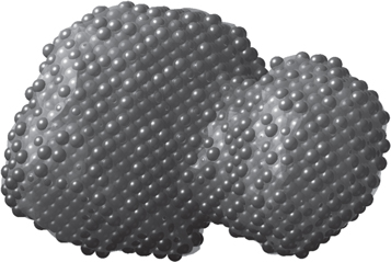
Figure 1. Shape model of 67P packed using our algorithm with spheres of radius rd = 100 m. Only sphere centers are required to be contained.
Download figure:
Standard image High-resolution image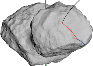
Figure 2. Shape model of 67P (SHAP5 v1.1) with the estimated Philae lander trajectory (Heinisch et al. 2016). The descent trajectory is shown in black. The "rebound" trajectory between first touchdown (TD1) and the collision with the Hatmehit crater wall (COL) at 16:20 UT, which we used in our simulations, is shown in red, while the trajectory after the collision is shown in blue. The green line is the spin axis of the comet.
Download figure:
Standard image High-resolution image2.2. Limited Interaction Distance Approximation
The number of spherical magnetic domains is roughly proportional to rd−3, where rd is the sphere radius, approximately the scale of coherent magnetization. Because of this scaling, sphere packing and field calculations become computationally expensive at small magnetization scales. To address this problem, we incorporated an approximation based on a maximum interaction distance, Dmax. Any point on the comet at a distance di > Dmax for all sampled points in a trajectory was ignored. Dmax was calculated as described below so that the combined magnetic field from the excluded region of the comet did not exceed a specified threshold Bmin.
We seek to estimate Dmax such that it it reduces computation time without introducing inaccuracies in the calculated field. We approach this by estimating an upper limit on the field of the ensemble of excluded dipoles. In particular, we estimate the field of the excluded dipoles as that of a single dipole with magnetic moment given by the vector sum of the magnetic moments of the excluded dipoles. From Heslop (2007), the probability density function for the magnitude, MN, of the vector resulting from the summation of N randomly oriented vectors of magnitude m is
Integrating this to find the expected magnitude yields
the familiar scaling relationship for a random walk with step-size m. Taking the magnetization scale, rd, as the sphere radius and assuming a specific magnetic moment, j, each dipole has a magnetic moment
where ρ is the density of cometary material. Note that N is a priori unknown for the volume of the body with r > Dmax. To save computation time, we estimate N without actually packing the body. We approximated N as the volume of the comet excluded (Vexcl) divided by the dipole volume:
where ϕ ≈ 0.74048 is the filling factor for close-packing of equal spheres. To calculate the resulting field from the spheres in the excluded volume, we approximated the field from the excluded volume as that of a single net dipole at one location with the following conservative assumptions: (1) the dipole has an orientation that creates the maximum possible field at the measurement location (the measurement point lies along the axis of the magnetic moment), (2) the net dipole is at a distance Dmax, and (3) the excluded volume is equal to the comet volume (Vexcl = V67P). The resulting magnetic field intensity of the excluded volume is found by combining Equations (4) and (5) with (3):
For a comet volume V67P = 18.7 ± 1.2 km3 (Preusker et al. 2015), this yields the scaling relation
Given the ROMAP upper limit of 0.9 nT on 67P's remanent field, Equation (7) shows that large portions of the comet can be ignored during many of our simulations. This dramatically improved the execution time of our simulations.
3. Simulation Results
We used the magnetization model described above to simulate the magnetic field generated by 67P. Our goal was to determine the maximum specific magnetic moment consistent with no detection of the comet's remanent field by Philae's ROMAP instrument (B ≲ 0.9 nT) for different spatial scales of coherent magnetization. We conducted simulations with magnetizations, j, from 10−6 to 10−1 A m2 kg−1 and magnetization scales, rd, ranging from 0.10 to 50 m.
In our simulations, we adopted a comet volume V67P = 18.7 ± 1.2 km3 and a bulk comet density of ρ = 535 kg m−3 (Preusker et al. 2015). We used the "SHAP5 version 1.1" shape model for 67P shown in Figure 2 (Jorda et al. 2016). The comet's topography is mapped by stereophotoclinometry—a technique that combines stereo images of the comet's surface taken under different illumination conditions. The resulting shape model consists of 3.1 million polygons and has an accuracy of ∼2 m (Jorda et al. 2016).
Philae was intended to land at one location on 67P, but instead rebounded from its intended landing site (initial touchdown, TD1) at 15:35 UT, collided with the Hatmehit crater wall (COL) at 16:20 UT, touched down again (TD2) at 17:25 UT, before finally coming to its final landing site (TD3) at 17:31 UT (e.g., Heinisch et al. 2016). We simulated 67P's remanent magnetic field along the reconstruction of the Philae trajectory provided by Heinisch et al. (2016) from first touchdown to the crater wall collision. We chose this section because it provides samples of the magnetic field along a ∼900 m swath of the comet's surface at low altitude (<100 m) and because the precise locations of the second and third touchdowns were uncertain at the time of our simulations. Given the extensive coverage at low altitude provided by the TD1 to COL portion of the trajectory, we do not expect that extending the modeled trajectory to TD3 would affect the results.
For runs using the limited interaction distance approximation described in Section 2.2, we used a conservative minimum field value of Bmin = 0.1 nT, or ∼10% of the 0.9 nT upper limit on the remanent field intensity. When using this approximation, smaller magnetizations (j) lead to smaller values of Dmax and correspondingly faster computation times. We therefore ran simulations at the lowest magnetization that would produce values near the ROMAP measurement uncertainty of 0.9 nT. Because the total field from all dipoles is simply the vector sum of the constituent dipole fields and  , once we have calculated the field for one choice of the magnetization, the results can, in principle, be linearly scaled to any other. However, when using the maximum interaction distance approximation, only scaling to smaller magnetizations preserves accuracy. We therefore limited scaling up to larger magnetizations to one order of magnitude, equivalent to the accuracy of requiring Bmin = 1 nT.
3.1. Full Trajectory Simulations
We performed simulations for rd at 50, 5, and 1 m over the entire rebound trajectory. Even for a magnetization of j = 1 × 10⁻⁶ A m2 kg−1 field intensities approaching 0.9 nT were recorded (Figure 3). Magnetic domain sizes of rd = 50, 5, and 1 m yielded maximum field intensities of 0.60, 0.53, and 0.53 nT, respectively.
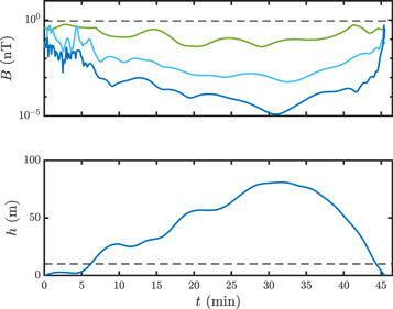
Figure 3. Simulated magnetic field and lander altitude from first touchdown (TD1, 15:35 UT) to the crater wall collision (COL, 16:20 UT) vs. time. Top: magnetic field magnitude assuming a specific magnetic moment of 10−6  . The green (upper), light blue (middle), and dark blue (bottom) lines correspond to magnetization scales (rd) of 50.0, 5.0, and 1.0 m, respectively. The dashed black line corresponds to the observational limit Bobs = 0.9 nT. Bottom: altitude (h) of the Philae lander above the comet's surface. The dashed black line is drawn at a height of 10 m.
Download figure:
Standard image High-resolution imageFigure 3 also illustrates the behavior of the magnetic field in different distance regimes. For a distance r ≫ rd, the lander is in the far-field and the comet's magnetic field is approximately that of a single dipole, so B ∝ r−3. In Figure 3, the simulation with rd = 1 m (dark blue) occupies this regime for altitudes h ≳ 10 m, indicated by the dashed black line.
Immediately after the bounce, and immediately before the collision, the simulated magnetic field intensities for the various values of rd converge, indicating that these simulations have entered a near-field regime. Here, the field at the lander is dominated by the nearest dipole, located at a distance r ∼ rd. In this regime, because the dipole's magnetic moment  , and the dipole field intensity Bdipole ∝ mr−3, the field intensity is independent of magnetization scale.
From these results, it is clear that, for the magnetization range of interest and rd ≤ 1 m, the lander will not measure significant magnetic fields in the far-field regime (h ≫ rd). We therefore conducted simulations at magnetization domain sizes smaller than 1 m on the subsections of the trajectory where we expected appreciable field intensity.
3.2. Low Altitude Simulations
To probe smaller magnetization scales, we restricted our simulations to the time immediately after first touchdown and immediately prior to the collision. We simulated magnetic field measurements for magnetization scales of rd = 0.25, 0.50, and 1 m at times when the lander was at an altitude h ≤ 10 m. For rd = 10 cm, we limited the simulation to times when h ≤ 1 m.
The maximum field intensities predicted post-touchdown (Figure 4) for j = 10−6 A m2 kg−1 and magnetization scales of 1 m, 50 cm, 25 cm, and 10 cm were 0.57 nT, 0.38 nT, 0.10 nT, and 0.14 nT, respectively. The corresponding values prior to the collision (Figure 5) were 0.88 nT, 0.61 nT, 0.76 nT, and 0.85 nT, respectively.
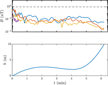
Figure 4. Simulated magnetic field and lander altitude immediately after first touchdown (TD1) vs. time after 15:35:16 UT. Top: magnetic field magnitude assuming a specific magnetic moment of 10−6  . The dark blue, red, orange, and purple lines correspond to magnetization scales (rd) of 1.0, 0.5, 0.25, and 0.10 m, respectively. The dashed black line corresponds to the observational limit Bobs = 0.9 nT. Bottom: altitude (h) of the Philae lander above the comet's surface.
Download figure:
Standard image High-resolution image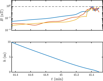
Figure 5. Simulated magnetic field and lander altitude immediately prior to collision with the crater wall (COL) vs. time after 15:35:16 UT. Top: magnetic field magnitude assuming a specific magnetic moment of 10−6  . The dark blue, red, orange, and purple lines correspond to magnetization scales (rd) of 1.0, 0.5, 0.25, and 0.10 m, respectively. The dashed black line corresponds to the observational limit Bobs = 0.9 nT. Bottom: altitude (h) of the Philae lander above the comet's surface.
Download figure:
Standard image High-resolution imageThe maximum field intensities from simulations at the same magnetization domain size (rd) for the component of the trajectory immediately after touchdown, prior to the collision, and over the entire rebound trajectory agree to within an order of magnitude. The largest discrepancies are at the smallest magnetization scales, where the lander is almost always in the far-field regime, so that the field intensity is highly sensitive to minor changes in geometry or altitude. Even for the lowest assumed magnetization (1 × 10⁻⁶  ), the simulated field intensities approach the 0.9 nT threshold imposed by the Philae observations, suggesting a very low upper bound on 67P's magnetization.
3.3. Maximum Magnetization
From the results of each of our simulations, we calculated the maximum specific magnetic moment consistent with no detection of the comet's remanent field:

where jmax is the maximum magnetization, jsim is the input magnetization for the simulation, Bobs = 0.9 nT, and Bmax,sim is the maximum value from the simulation. The maximum simulated field value in a simulation occurs at or near the point of lowest altitude, where the limited accuracies of the shape model (∼2 m) or reconstructed trajectory may play a role. However, this is not a significant limitation because the estimated maximum magnetizations are driven by the altitude of closest approach, and not its precise location. Because we know from the reconstruction of the trajectory (Heinisch et al. 2016) that ground contact occurred, the inaccuracy of the shape model is not significant.
The spherical domains in our simulations have a fixed magnetization, implying that they each are composed of the same ferromagnetic materials that are intimately mixed at spatial scales much smaller than the sphere radius. However, 67P is composed of both dust and non-magnetic ice. To determine the magnetization limit of the dusty material, we incorporated the dust-to-ice mass ratio, ξ:
The dust-to-gas mass ratio measured for 67P is 4 ± 2 (Rotundi et al. 2015). Additionally, experiments on silica and ice pebble compression during collision coupled with simulations of pebble-pile formation for 67P suggest that the measured porosity requires 3 ≲ ξ ≲ 9 (Lorek et al. 2016). We therefore conservatively (i.e., higher inferred magnetization) assume ξ = 3. The results for each simulation are shown in Figure 6. For rd = 0.5 m, the average of the maximum magnetizations from our simulations is 2.6 × 10⁻⁶  . The analogous value from Auster et al. (2015), corrected with the updated bulk density , the new constraint on the measured field intensity (Heinisch et al. 2018), and ξ = 3, is 1.6 × 10⁻⁵
  . At domain sizes smaller than one meter, we obtained jmax ∼ 5 × 10⁻⁶
  , while at scales of one meter and larger, jmax ∼ 2 × 10⁻⁶
  . The values are in broad agreement with the low specific magnetic moment inferred for 67P by Auster et al. (2015).
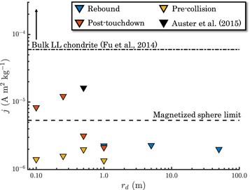
Figure 6. Maximum specific magnetic moment, j, inferred for cometary material at a range of magnetic domain scales (rd) from our simulations and the value from Auster et al. (2015). The inverted triangles indicate that these values are upper limits. The upper dashed line at 6 × 10⁻⁵  is the value for demagnetized matrix material from Semarkona (Fu et al. 2014b). The lower dashed line at 5.4 × 10⁻⁶
  is the maximum magnetization of a sphere consistent with a 0.9 nT field on its surface. Nearly all of our simulations require a magnetization less than this value.
Download figure:
Standard image High-resolution image3.4. Implications for Accretional Detrital Remanent Magnetization on 67P
If 67P retains ADRM, then, over a given region, magnetic grains that were accreted during the formation of the comet would have nearly aligned magnetic moments. The alignment of these moments results in material that is approximately uniformly magnetized, producing a bulk specific magnetization comparable to that of the individual grains, jbulk ∼ jgr. The length scale (rd in our model) of these regions is poorly constrained by theory and could, depending on the details of 67P's formation, range from several times the average grain size (rd ∼ 5 cm) to the size of the entire comet (rd ∼ 2 km). Conversely, random orientation of magnetic grains results in a specific magnetization for bulk material that is significantly less than the grain magnetization, jbulk ∼ (rgr/rd)3/2(ρgr/ρbulk)1/2jgr. If the maximum jbulk permitted by the Philae measurements for a given value of rd is below that expected for uniform magnetization (i.e., the magnetization of individual grains) then this suggests either that ADRM is not recorded on 67P or that ADRM operates with low efficiency. ADRM may have lower than perfect efficiency as a result of spatial or temporal variations in the aligning magnetic field or grain misalignment during accretion.
The Philae data do not provide a significant constraint on the magnetization of small (≲1 mm) grains on 67P, but samples of other solar system bodies can provide a range of plausible values. Studies of material returned from the JFC 81P/Wild ("Wild 2") by the Stardust mission show that the rocky component of JFCs is similar to primitive ordinary chondritic material (Brownlee et al. 2012). Meteorite measurements have shown that chondritic material can possess a remanent magnetization spanning from ∼4 × 10⁻⁵ to ∼1 × 10⁻¹  (e.g., Terho et al. 1993). Note, however, that many chondrites with moments >0.01
  were likely remagnetized by collectors' hand magnets (Weiss et al. 2010). Chondrules and millimeter-sized bulk samples of the Allende CV carbonaceous chondrite tend toward the low end of this range, 10−5–10−4
  (e.g., Fu et al. 2014a). Finally, pieces of the matrix of the Semarkona LL3.00 ordinary chondrite that have been completely demagnetized by alternating fields in the laboratory have a specific magnetization of ≳6 × 10⁻⁵
  (Fu et al. 2014b).
In comparison to measurements of meteorite samples, 67P is strikingly non-magnetic—permissible values of the bulk magnetization of 67P on scales ≥10 cm are generally an order of magnitude less than even the lowest values reported from meteoritic materials. This suggests either that 67P does not contain regions of coherent magnetization on these scales from ADRM in the areas where Philae made ground contact, or that ADRM operates with a low alignment efficiency, at most ∼10% and possibly much lower.
4. Accretional Detrital Remanent Magnetization in the Outer Nebula
The Philae-derived constraints on the magnetization of 67P are inconsistent with the presence of ADRM with an alignment efficiency ≳10% on length scales ≥10 cm. We cannot distinguish between low-efficiency ADRM and the total absence of ADRM, but both conditions suggest the failure, to a large degree, of at least one of the conditions necessary for acquisition and preservation of ADRM (Figure 7). For the following analysis, we therefore assume that ADRM is not recorded on 67P. There are three main requirements for ADRM to be recorded and preserved: the grains must have been aligned by the background field during accretion, they must be accreted to the comet while remaining aligned, and they must not be dis-aligned in subsequent processing on the comet by impacts or aqueous alteration. We discuss these requirements in Sections 4.1, 4.2, and 4.3, respectively.

Figure 7. Schematic diagram of planetesimal formation with acquisition of accretional detrital remanent magnetization. Comet formation must occur (1) through the collapse of a pebble cloud composed of (2) ∼millimeter-sized pebbles (3) in the presence of a field intense enough to enforce pebble alignment.
Download figure:
Standard image High-resolution image4.1. Grain Alignment
The first stage in ADRM acquisition is the alignment of nebular grains to the background magnetic field. We review the requirements for grain alignment as described by Fu & Weiss (2012), adapting them where necessary for conditions in the outer solar nebula. The "compass-needle" mechanism of grain alignment described here is distinct from the theory of radiative grain alignment, which is more commonly discussed in the protoplanetary disk literature (e.g., Tazaki et al. 2017; Hull et al. 2018). In radiative alignment torque theory, a spinning paramagnetic grain acquires a magnetic moment parallel to its spin axis through the Barnett effect. Grain alignment then proceeds from the precession of a spinning grain's angular momentum vector about the direction of either the magnetic field or the anisotropic radiation field, depending on the relative strengths of the magnetic and radiative torques. Over ∼10–100 precession periods, the angular momentum vector becomes aligned with the precession vector (Lazarian & Hoang 2007).
The compass-needle mechanism of grain alignment discussed in this paper differs from radiative alignment in two ways. First, alignment of a grain occurs after the grain has been brought to near rotational rest by interaction with nebular gas. Second, the magnetic moments of these grains are produced by the presence of magnetized ferromagnetic inclusions, not grain rotation. As a result, these grains possess magnetic moments that are orders of magnitude larger than those produced through the Barnett effect. Additionally, the magnetization direction for these grains is independent from the shape of the grain. As a result, grains that are aligned to the nebular field by this mechanism should have no preferred orientation of their long axes and are therefore not expected to produce a polarized emission signature. Grain alignment in the compass-needle framework requires first that the torque exerted by the magnetic field be stronger than other randomizing torques on the ferromagnetic grain. Second, for the grain to remain aligned, the time between collisions, which disrupt the grain orientation, must be significantly greater than the time required to bring the grain back into alignment.
In these calculations, we adopt the minimum-mass solar nebula model from Hayashi (1981) with the gas temperature (Tg), gas density (ρg), and gas scale height (Hg) defined as
where a is the heliocentric distance in the midplane of the nebula. The scale height Hg defines the exponential vertical profile of the gas at a given heliocentric distance: at a height z above the disk midplane,  . The H/He nebular gas has a mean molecular weight of μ = 2.34 u.
4.1.1. Grain Torques
Magnetic Torque—For grain alignment, the magnetic torque must exceed other randomizing torques on the grain. Depending on the grain size, the particular non-magnetic torque that dominates varies (Figure 8).
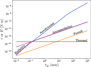
Figure 8. Non-magnetic torques or energies affecting nebular grains of varying radii (rgr) at a = 20 au. The aerodynamic torque shown here assumes long grains in a turbulent nebula (χ = 2, α = 10−2). For more accurate comparison with the torques, the plotted thermal energy is (10/π)2kBTg rather than simply kBTg (see Equation (12)). The small variations in the calculated aerodynamic torque at very small grain sizes are caused by numerical instabilities during integration.
Download figure:
Standard image High-resolution imageThe magnetic torque exerted by a field with intensity B on a spherical grain with a specific magnetization jgr is

where rgr and ρgr are the radius and density of the grain, respectively. We assume ρgr = 2000 kg m−3 in all our calculations. We adopt a conservative value of jgr = 10−5  for the grain magnetization (see Section 3.3).
Brownian Motion—Very small grains are subject to randomization through rotational Brownian motion. Following Fu & Weiss (2012), we consider a grain to be misaligned when the thermal energy of rotation (kBT/2, where kB is the Boltzmann constant) exceeds the difference in magnetic potential energy for an aligned grain and one misaligned by an angle θ = π/10. Using the small-angle approximation, the threshold for alignment is then
Solving this inequality for the magnetic field intensity (B) and substituting into Equation (11), the magnetic torque required to align grains against Brownian randomization is  .
.
Aerodynamic Drag—Grains in the solar nebula experience aerodynamic drag as a consequence of their motion relative to the nebular gas. The drag regime depends on the ratio of the mean free path of gas molecules to the size of the grain. This ratio is defined as the Knudsen number,
where ng = ρg/μ is the gas number density and σ = 2 × 10⁻¹⁵ cm2 is the collision cross section of H2 (Nakagawa et al. 1986). We define grains with Kn > 1/8 to be in the free molecular (FM) drag regime, where the mean free path is large compared to the grain size. All the grains of interest in this study fall into this regime. The net torque on a grain in an FM flow is determined by integrating the effects of gas molecule collisions on each surface element of the grain over the entire surface area. As in Fu & Weiss (2012), we assume the grains are prolate ellipsoids with an aspect ratio χ, defined as the ratio of the lengths of the semimajor and semiminor axes. For comparison to other torques, we consider rgr as the semiminor axis, so that χrgr is the semimajor axis. Expressions for the FM torque on an arbitrary convex figure of revolution, assuming a Maxwellian velocity distribution for the gas and thermal equilibrium between the gas and dust grain, are provided by Equation (3) from Ivanov & Ianshin (1980). We use their expression for Mx and assume an angle of π/4 between the long axis of the grain and the gas velocity vector (see Appendix B for details).
The relative velocity between the gas and dust grain has two components. First, the systemic drift velocity, caused by sub-Keplerian motion of the gas, and, second, velocity differences caused by turbulence in the gas. We determine the total systemic velocity from the radial (u) and transverse (w) velocity components,  , where u and w are determined by solving Equations (15) and (20) in Weidenschilling (1977), as detailed in Appendix B.
The relative velocity induced by turbulence is
StL is the Stokes number relative to the largest eddy, Re is the flow Reynolds number, and vg is the mean square of the turbulent gas velocity (Cuzzi & Hogan 2003). StL is given by the ratio of the stopping time of a grain due to gas drag to the overturn time of the largest eddy, which is comparable to the orbital period:
where  is the thermal velocity of the gas (Nakagawa et al. 1986). The Reynolds number is given by
where η ∼ ρgvth/(ngσ) = vth/(μσ) is the dynamic molecular viscosity of the nebular gas and  and
and  (Cuzzi et al. 2001). The latter two expressions are derived from the assumption of an α-disk model, where angular momentum transport in the disk is assumed to be driven by a turbulent viscosity ∼αvthHg. Values for the dimensionless turbulence parameter α used here are 10−4 and 10−2, corresponding to either a quiescent or a turbulent nebula. To find the total relative velocity between grains and the nebular gas, we make the conservative assumption that
  instead of adding the components in quadrature.
Accommodation Torque—Grains in the nebula can also experience torques as a consequence of surface heterogeneities. Differences in the efficiency of momentum transfer (or accommodation) during gas molecule collisions across the surface of a grain can result in a rotation rate higher than expected from random impacts of gas molecules (Purcell 1979). The magnitude of the effective torque, from Equation (14) of Purcell, is
where δ is the magnitude of the variation in the accommodation coefficient, s is the length scale over which the accommodation varies, and  describes the difference between the grain temperature (Ts) and the gas temperature and is parameterized by ηa = ΔT/Tg.4
Following Purcell (1979) and Fu & Weiss (2012), we adopt s = 10−7 m, and the conservative values δ = 0.1 and ηa = 1.
describes the difference between the grain temperature (Ts) and the gas temperature and is parameterized by ηa = ΔT/Tg.4
Following Purcell (1979) and Fu & Weiss (2012), we adopt s = 10−7 m, and the conservative values δ = 0.1 and ηa = 1.
Purcell Torque—Like the accommodation torque, the Purcell torque also arises as a consequence of variations in the properties of the grain surface. At certain sites on the grain, the binding energy of incoming hydrogen atoms is enhanced so that they become more tightly bound to the grain. The arrival of a second hydrogen atom can then result in recombination and the ejection of the resulting hydrogen molecule, causing a reaction force on the grain. The random distribution of these sites of hydrogen formation and ejection over the surface of the grain gives rise to a torque
where γ is the fraction of inbound hydrogen atoms that are ejected as molecules, nH is the number density of hydrogen atoms, ν is the number of enhanced sites on the grain, and Eej = 0.2 eV is the mean kinetic energy with which the molecule is ejected (Purcell 1979, Equation (19)). We adopt γ = 0.2 and ν = 100 × (rgr/10−7 m)2 from Fu & Weiss (2012) as values appropriate for the solar nebula. At the temperatures expected in the midplane region where 67P likely formed, the gas is dominated by molecular hydrogen, so that the abundance of atomic hydrogen is nH/ng ≲ 10−4 (e.g., Glassgold et al. 2009). We therefore take nH/ng = 10−4 as a conservative assumption in our calculations. Given the weak magnitude of the Purcell torque compared to other effects across the grain sizes of interest, the uncertainty in these parameters does not affect our results.
Radiative Torque—The final effect we consider is the radiative torque, affecting irregularly shaped grains in a uniform radiation field. From Equation (29) of Fu & Weiss (2012) the approximate magnitude of the torque is

where  is the mean wavelength of the incident radiation, QΓ is an efficiency coefficient that depends on the grain size, and urad is the volumetric energy density of the radiation. In the interior of the disk, the radiation field is dominated by thermal emission from cool grains (e.g., Tazaki et al. 2017). Following Fu & Weiss, we therefore adopt
  , QΓ ∼ 1 for
  and
and  for
for  , and a radiation density
where c is the speed of light and h is Planck's constant. Following Chiang & Goldreich (1997), we assume thermal equilibrium between the dust and gas in the disk midplane, Tgr ∼ Tg. This is a conservative choice, because it results in an overestimate of the radiation density by roughly an order of magnitude when compared to the more sophisticated model of Tazaki et al. (2017).
Considering all the torques above, we determine the magnetic field intensity required for the magnetic torque (Equation (11)) to be the strongest torque acting on grains of varying size (Figure 9). This provides a lower bound on the magnetic field intensity required to magnetically align the grains. For grains with rgr ≲ 0.1 mm we find that alignment is determined by competition between Brownian motion and the magnetic torque, while for rgr ≳ 0.1 mm the dominant non-magnetic torque is aerodynamic drag. We consider two cases for aerodynamic drag: a lower bound case with nearly circular grains and a quiescent nebula (χ = 1.1 and α = 10−4), and an upper bound case with prolate grains and a highly turbulent nebula (χ = 2 and α = 10−2). The required field intensity is strongly dependent on the grain radius, but even in the higher drag scenario, the magnetic torque will control alignment of millimeter-sized grains for fields B ≳ 1 μT.
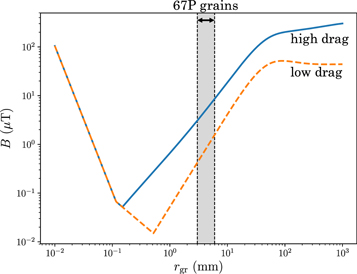
Figure 9. Required magnetic field intensity for the magnetic torque to control the alignment of grains with radii between 0.01 mm and 1 m in the solar nebula at 20 au. The two curves give the magnetic field intensity at which the magnetic torque equals the largest non-magnetic torque from Figure 8. The gray shaded region indicates the approximate range of grain sizes found on 67P (e.g., Blum et al. 2017). The solid blue line corresponds to elongated grains in a turbulent nebula (χ = 2, α = 10−2) and the dashed orange line represents nearly circular grains in a quiescent nebula (χ = 1.1, α = 10−4).
Download figure:
Standard image High-resolution image4.1.2. Grain Alignment and Collision Timescales
Even when the magnetic torque dominates over other forces acting on nebular grains, alignment is disrupted by collisions with other grains. These collisions randomize the orientation and spin up the grains. When a grain is rapidly spinning (ω ∼ 102 s−1), the rotational energy is much greater than the work done by the magnetic torque in one revolution, making direct realignment impossible and causing the grain to instead precess about the field direction (Fu & Weiss 2012). Realignment is therefore a two-stage process. First, on a timescale tprec, the grain must shed its rotational energy through gas drag. Subsequently, the magnetic torque can reorient the grain, and the grain's magnetic moment oscillates about the field direction, with the gas drag now serving to damp the oscillation. This damping occurs on a timescale of tdrag. Grain alignment in the solar nebula requires that the time between collisions be much longer than the time required to de-spin and realign the grain: tcoll ≫ talign = tdrag + tprec. From Fu & Weiss (2012), the collision, drag, precession, and alignment timescales are

where vrel is the relative velocity between grains in the nebula, ρs is the density of solids in the nebula, and ω0 is the initial angular velocity of a grain after a collision. The factor f represents the efficiency of momentum transfer during gas molecule collisions and is assumed here to be 1. For conditions in the outer solar nebula, we find that tprec ∼ 10 tdrag, so that talign is roughly an order of magnitude greater than tdrag. This conclusion is insensitive to assumptions about the magnetic field strength and grain magnetization owing to the logarithmic dependence on these factors. Fu & Weiss (2012) show that in the solar nebula tcoll ≫ talign for grains with rgr ≲ 10 cm, suggesting that, if the magnetic torque dominates grain alignment, small grains will be aligned to the background field most of the time.
4.1.3. Upper Limit on Field Intensity
If the absence of ADRM on 67P is due to the failure of grain alignment in the solar nebula, then the calculated field intensity at which the magnetic torque dominates other forces (Figure 9) provides an upper bound on the nebular field intensity at the time and location of 67P's formation.
The location of 67P's formation is not well constrained. Comets are believed to have formed in a disk of icy planetesimals in the region of ∼15–45 au before being scattered by interactions with the giant planets to form the scattered disk and the Oort cloud (Fernandez & Ip 1981; Brasser & Morbidelli 2013; Johansen et al. 2014). Additional clues to the formation environment come from 67P's ice and volatile inventory. The release of volatiles from 67P is consistent with the decomposition of H2O clathrates, suggesting that at least some of the water ice on 67P is not amorphous (Rubin et al. 2015; Luspay-Kuti et al. 2016; Mousis et al. 2016a, 2016b). Crystalline ice and clathrates are expected to form in the solar nebula through the vaporization of amorphous ice at temperatures of ∼150 K followed by condensation as the disk cools, requiring formation at distances ≲30 au (Willacy et al. 2015). Results from the Stardust mission, however, suggest substantial radial transport of material prior to or during the epoch of comet formation (Brownlee et al. 2012), so the presence of these ices may not directly reflect the formation location. Given these uncertainties, we calculate the minimum field intensity required to enforce grain alignment assuming a formation location of 15–45 au. For a given grain size, the results show that there is little change in calculated field intensities over this range of heliocentric distances.
However, the required field intensity is strongly influenced by the assumed size of the grains that agglomerated to form 67P (Figure 9). As discussed below (Section 4.2), this value is in turn highly dependent on the assumed mechanism by which the comet formed. Multiple lines of evidence, including 67P's thermal inertia, porosity, and surface features, suggest that 67P is composed largely of pebbles with a characteristic radius of 3–6 mm (Fulle et al. 2016; Poulet et al. 2016; Blum et al. 2017). Assuming, for the moment, that this approximates the size of nebular grains that accreted to form 67P, the absence of ADRM requires a magnetic field intensity B ≲ 1 μT for rgr = 1 mm and B ≲ 3 μT for rgr = 3 mm (Figure 10).
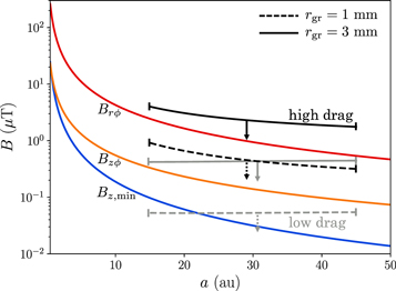
Figure 10. Theoretical predictions of nebular field intensity and maximum field intensity values consistent with no ADRM on 67P as a function of heliocentric distance. The three theoretical curves are, in decreasing intensity, the predictions for radial–azimuthal (rϕ) coupling of the instantaneous magnetic field (Bai & Goodman 2009, Equation (16)), vertical–azimuthal (zϕ) coupling of the instantaneous field (Bai & Goodman 2009, Equation (7)), and the minimum stable net vertical (z, min) field (Bai 2015, Equation (14)). We assume an accretion rate of 10−8 M⊙ yr−1. The 67P constraint is plotted using dotted and solid lines, which correspond to assumed grain radii of 1 and 3 mm, respectively. These lines are plotted in black for elongated grains in a turbulent nebula (χ = 2, α = 10−2) , and in gray for nearly circular grains in a quiescent nebula (χ = 1.1, α = 10−4).
Download figure:
Standard image High-resolution imageThe predicted alignment timescale for ferromagnetic grains (≲1 yr) is much shorter than the timescale for variation in the outer disk magnetic field found in simulations (∼10–100 yr) (e.g., Bai 2015). Absence of grain alignment on 67P therefore constrains the instantaneous magnetic field in the outer disk, not the weaker time-averaged net field (so that the orange and red curves in Figure 10 are the relevant curves to be compared to the Philae constraints). Our derived limits on field intensity are broadly consistent with theoretical predictions of the instantaneous magnetic field intensity required to drive stellar accretion at the assumed rate of ∼10−8 M⊙ yr−1 (red and orange lines in Figure 10).
Observations of (sub)millimeter thermal emission from dust grains in other protoplanetary disks offer a complementary way to measure magnetic field intensities. The polarization of this emission is related to the alignment of grains with sizes comparable to the wavelength, so the intensity and morphology of the observed polarization can indicate the mechanism that is controlling grain alignment. Recent observations of the protoplanetary disks around HL Tau and IM Lup show a pattern of polarization consistent with either self-scattering by unaligned dust grains, or radiative, not magnetic, alignment of dust grains (e.g., Kataoka et al. 2015, 2017; Yang et al. 2016; Stephens et al. 2017; Tazaki et al. 2017; Hull et al. 2018). Tazaki et al. (2017) estimate that a magnetic field intensity ≳13 μT is required for magnetic alignment to supersede radiative alignment for millimeter-sized grains at 50 au, consistent with, but less restrictive than, the upper bounds on the field intensity we infer from 67P. Tazaki et al. (2017), however, primarily considered non-magnetic grains or grains with super-paramagnetic inclusions. We consider grains with ferromagnetic inclusions, which can have much larger magnetic moments and can therefore become aligned at lower field intensities. Additionally, present-day observations of polarized emission from protoplanetary disks have typical resolution of ∼10 au, making it difficult to probe the inner regions of the disk where comet formation likely occurred. The 67P measurements therefore provide both a tighter constraint on the magnetic field and insight into a region of the disk that is difficult to access with current astronomical measurements.
4.2. Formation Mechanism
Even under conditions where nebular grains are aligned to the background field, the mechanism by which these grains accrete to form a comet is critical for determining whether ADRM is possible. For grain alignment to be preserved and produce a magnetic record, the grains must be directly accreted by the comet while maintaining alignment.
There are two main hypothesized mechanisms for the formation of comets: hierarchical growth and pebble cloud collapse. If comets undergo hierarchical growth, forming gradually through collisional coagulation of increasingly large aggregates (e.g., Weidenschilling 1997; Davidsson et al. 2016), then ADRM is likely impossible or extremely limited in spatial scale. For plausible magnetic field intensities, the orientation of grains ≳1 cm in radius will be dominated by other factors, so that pairwise collisions of particles larger than this size will produce random mutual orientations of their magnetic moments. This scenario could explain the absence of ADRM on 67P at spatial scales ≥10 cm even in the presence of an intense background magnetic field.
Alternatively, recent modeling has demonstrated that the concentration of nebular solids through the streaming instability (Johansen et al. 2007), followed by the gentle gravitational collapse of the resulting cloud of millimeter- or centimeter-sized grains, can produce comet-like planetesimals matching the observed density, porosity, and tensile strength of comets (Blum et al. 2014; Wahlberg Jansson & Johansen 2014, 2017; Lorek et al. 2016). The detection of millimeter-sized pebbles on 67P, by direct imaging among other techniques, combined with the primitive nature of cometary material and the preservation of fluffy fractal dust aggregates, has been taken as evidence that 67P formed directly from the pebbles observed today (Fulle et al. 2016; Poulet et al. 2016; Blum et al. 2017; Fulle & Blum 2017). Blum et al. (2017) and Fulle & Blum (2017) argue that this evidence disfavors hierarchical growth models, which would compress fluffy fractal dust particles and would result in a range of grain sizes from small grains (∼10 μm) to larger aggregates, instead of the observed characteristic size of a few millimeters. In the pebble-pile scenario, because 67P directly incorporates millimeter-sized grains as it accretes, the absence of ADRM cannot be easily explained by the formation mechanism alone, but would also require the background field to be weak.
A possible factor limiting ADRM formation in the pebble pile is the repeated grain collisions in the pebble cloud preventing grain alignment (see Section 4.1.2). This is because the pebble cloud is much denser than the background nebula we had previously considered. To determine whether alignment can be maintained in these overdense regions, we recalculate the collision and alignment timescales (Equations (21) and (23)) for conditions at the start of cloud collapse. Following Lorek et al. (2016) and Wahlberg Jansson & Johansen (2014), the initial pebble cloud has uniform density, a mass M67P ≈ 9.982 × 10¹² kg (Pätzold et al. 2016), and a radius equal to its Hill radius, RH. We assume millimeter-sized grains, a formation distance of 20 au, a background field intensity B = 0.1 μT, and grain magnetization jgr = 10−5  . We take the velocity dispersion to be
  , where the virial velocity is
  , and we conservatively estimate that the initial grain rotation rate after a collision is given by ω0 = vrel/rgr. We find that the criterion for alignment is still satisfied in the initial pebble clouds: tcoll ≈ 19 yr ≫ 4 yr ≈ talign.
As the cloud collapses, grain collisions continue. Initial models (Wahlberg Jansson & Johansen 2014) assumed a homogeneous particle size distribution in the cloud, leading to a steady increase in cloud density until solid density was reached. Under these conditions, the collision timescale rapidly decreases at the end of collapse, possibly randomizing grain orientations. More recent models (Wahlberg Jansson & Johansen 2017), which radially resolve the accreting planetesimals and include the effects of gas drag, suggest that comet-sized planetesimals may form through the rapid accretion of a core followed by the protracted accretion of a remnant low-density cloud. Because of the low density, collision rates during the end stage are low, so these grains may be able to maintain alignment to a background field. A caveat is that even these updated models lack important physics, including the rotation of the collapsing cloud. In summary, the absence of ADRM on 67P could be explained by a hierarchical growth model, but if comets form instead through the gentle gravitational collapse of a cloud of pebbles, then the formation mechanism alone may not explain the lack of magnetic alignment of 67P's constituent grains.
4.3. Subsequent Alteration
Significant post-formation restructuring would also provide a natural explanation for the observed lack of ADRM on 67P. There is some evidence that, rather than primordial objects, comets may be collisional rubble piles, forming from the re-accretion of material from a larger parent body (Morbidelli & Rickman 2015; Rickman et al. 2015). Others argue that 67P's high porosity, low tensile strength, abundance of supervolatiles, absence of aqueous alteration, and preservation of fractal dust particles require a primordial origin (Davidsson et al. 2016; Blum et al. 2017; Fulle & Blum 2017). Recent modeling of collisions, however, has shown that at least some primitive properties of cometary material can be preserved through significant collisional restructuring, including during disruption of the parent body and subsequent re-accretion (Jutzi et al. 2017; Schwartz et al. 2018). These scenarios do not predict global crushing or compaction on sub-meter scales, which would be difficult to reconcile with the retention of supervolatiles and high porosity, although these effects are well below the ∼10 m resolution limits of the models. Collisions may be capable of erasing ADRM on ≳10 m scales, but magnetization on ≲1 m scales may persist, even if the bulk structure of 67P is not primordial.
Outgassing, sublimation of volatiles, erosion, and sedimentation may all change the structure of 67P on smaller scales, resulting in the scrambling of grain orientations and loss of ADRM. Because our results are most sensitive to the measurements closest to the comet's surface, a regolith layer ∼1 m thick could mask ADRM if it were recorded on only ∼10 cm scales. Much thicker regolith layers are required, however, to mask magnetic coherence on greater length scales. The Philae data include low-altitude magnetic field measurements at multiple contact points on the nucleus. The initial touchdown location was in a region with an estimated 20–30 cm thick layer of granular regolith and meter-sized pits overlying more consolidated material (see discussion of "pitted plains" in Birch et al. 2017), while the final touchdown location is believed to be primordial, displaying a relatively dust-free landscape with nearby blocks and boulders and stratified terrain (Lucchetti et al. 2016; Poulet et al. 2016). The remanent field intensity is ≤0.9 nT at all contact points, regardless of the thickness of regolith or apparent degree of alteration. Birch et al. (2017) propose that observed comet nuclei display a range of alteration, with smoother terrain present on more altered comets. They argue that 67P displays more primordial morphology than most other JFCs. If the observed radial-layered structure is also primordial (Massironi et al. 2015), then this also places tight constraints on the degree of structural alteration.
Surface processes may be able to erase, or mask, ADRM on 67P if it was only ever acquired on small length scales. By contrast, if 67P, or its parent body, acquired large-scale ADRM during formation, a combination of collisions and surface processing would be required to remove it.
ADRM could also be removed by the remagnetization of ferromagnetic minerals after accretion. Processes that would be capable of remagnetizing 67P include heating to temperatures exceeding several hundred kelvin, aqueous alteration, or impact shocks exceeding ∼1 GPa (Gattacceca et al. 2007). However, these conditions are more extreme than those predicted by models of collisional rubble piles (e.g., Jutzi et al. 2017; Schwartz et al. 2018), and 67P shows no evidence of the extensive and widespread heating, aqueous alteration, or large shocks that would be required to demagnetize it over the entire region surveyed by Philae (e.g., Davidsson et al. 2016; Fulle & Blum 2017). We therefore consider this an unlikely explanation.
5. Conclusions
In this paper we present updated constraints on the maximum specific magnetic moment for cometary dust on 67P. Our simulations used a reconstructed trajectory for the Philae lander (Heinisch et al. 2016) and the 67P shape model (Jorda et al. 2016) to extend the work of Auster et al. (2015). We find that mass-specific magnetizations of ≲5 × 10⁻⁶  are required for all assumed magnetic coherence length scales ≥10 cm. These results show that either ADRM is not present on 67P or it is recorded with very low efficiency, at most ∼10%. This observation supports multiple interpretations: (1) 67P formed in a weak background magnetic field, consistent with recent observations of protoplanetary disks that show polarized emission from dust grains, which is inconsistent with their alignment with the disk's magnetic field (Section 4.1); (2) 67P's formation process did not permit acquisition of ADRM, either because it did not form as a pebble-pile planetesimal or because pebble-pile formation produces collisions of dust grains at too high a velocity and too frequently for magnetic alignment (Section 4.2); (3) 67P has been sufficiently altered through collisions and surface processes that any accretional magnetic signature has been erased (Section 4.3). We cannot definitively exclude any of these explanations, but based on the evidence for direct accretion of millimeter-sized grains and the degree of processing required to remove ADRM, we favor the first hypothesis.
If the weakness of the magnetic field is responsible, the absence of ADRM requires a background field intensity ≲3 μT during comet formation. This provides the first observational constraint on the magnetic field in the outer solar nebula. This constraint is consistent with expectations from models of magnetic fields driving turbulence in the solar nebula, but the degree of uncertainty prevents us from differentiating between the proposed mechanisms. The low magnetic field intensity in the outer nebula indicates that other samples derived from the outer solar system should record low paleointensities (≲3 μT) for the nebular field, opening up the possibility of using paleomagnetic techniques as a proxy for formation distance. If a body in the outer solar system is highly magnetized, this likely cannot be caused by the nebular field and may instead be evidence for an internal dynamo. Continued paleomagnetic studies of meteorite samples will test ADRM theory by searching for the magnetic alignment of grains that have not been remagnetized since accretion. In addition, laboratory measurements of returned 67P samples (Squyres et al. 2018) could likely definitively distinguish between the three hypotheses described above, and thereby place stringent constraints on the nebular field and accretion process in the comet-forming region.
We thank the anonymous referee for comments that significantly improved the manuscript. We additionally thank X. Bai, R. Fu, and J. Bryson for useful discussions. We gratefully acknowledge support from the NASA Emerging Worlds program (grant No. NNX15AH72G) , the U.S. Rosetta program (CREI 1576768), and Thomas F. Peterson Jr.
Software: Astropy (Astropy Collaboration et al. 2013), matplotlib (Hunter 2007), NumPy (Van Der Walt et al. 2011), SciPy (Jones et al. 2001).
Appendix A: Sphere Packing Algorithm
Our technique for packing a model of arbitrary shape with spheres of uniform size uses a slightly modified version of a standard technique in computational geometry known as ray casting. Ray casting determines whether a given point is contained inside a shape by computing all the intersections of a ray drawn from the given point with the boundary of the shape. If and only if the point is contained in the shape, the ray will cross the shape boundary an odd number of times.
To pack the shape model of the comet, we begin by constructing an axis-aligned bounding box around the comet (i.e., the length, width, and height of the box are aligned with the x, y, and z axes of the coordinate system). We then define a hexagonal close-packed (hcp) lattice of spheres of equal size filling the bounding box. Hexagonal close-packing produces a packing density of  , which is the highest achievable by any arrangement of spheres. We then iterate through the hcp lattice of spheres, filling the bounding box to remove those falling outside the shape model using ray casting. The computational cost of this procedure increases with the resolution of the shape model, which determines the number of facets of the shape model that a ray might intersect, and the number of spheres to be tested, which determines the number of sphere centers to check and depends on the sphere radius (
 ).
).
An hcp lattice has A–B–A–B layering, i.e., if we start with a layer in the x–y plane, then alternating layers of spheres have the same x and y coordinates for their centers, with only a z offset. Specifically, the coordinates of sphere centers can be written as
where rd is the sphere radius, and i, j, k are indices indicating lattice position with respect to the x, y, and z axes. For values of k with the same parity (i.e., k = 0, 2, 4, ... or k = 1, 3, 5, ...) all spheres with the same i and j indices will have the same x and y coordinates. A ray cast in the z-direction from a sphere in the bottom layer (k = 0) will intersect the centers of all the spheres with the same i and j indices and even-numbered k. This allows us to determine the disposition of all the spheres in the bounding box by performing ray-casting calculations from only the k = 0 and k = 1 layers of the lattice, reducing the scaling of the computation time with sphere size to roughly ∝rd−2.
Appendix B: Aerodynamic Torques on Nebular Grains
We describe here in more detail the calculations of the aerodynamic torque from Section 4.1.1. We begin with the systematic grain velocity, which we take as  where u and w describe the radial and transverse velocities of the grain with respect to the gas. The velocities are determined by solving Equations (15) and (20) from Weidenschilling (1977):
where Vg is the transverse orbital velocity of the gas, Vk is the circular Keplerian velocity, Fd is the drag force, and mgr is the grain mass. The transverse orbital gas velocity is less than the Keplerian velocity as a consequence of pressure support from the gas in the disk and is given by  , where n = 13/4 is the exponent for the dependence of the gas pressure on semimajor axis, P ∝ a−n (Weidenschilling 1977). The drag-to-momentum ratio of the grain can be calculated assuming the Epstein drag law, Fd/(mgrvsys) = −ρgvth/(ρgrrgr). With this approximation, we can directly solve Equations (26) and (25) to obtain u and w.
To obtain the aerodynamic torque, we combine the systemic velocity with the turbulent velocity,  , and use this velocity in the torque calculation provided by Ivanov & Ianshin (1980). In their paper, they provide analytic expressions for the aerodynamic torque on a convex figure of rotation in an FM flow, which we reproduce here with some modifications to match the nomenclature in this paper. They define a body-fixed right-handed Cartesian coordinate system with the z-axis along the long axis of the grain and the flow velocity in the y–z plane (i.e., orthogonal to the x-axis), and a corresponding cylindrical system with radius R, oriented orthogonally to the z-axis, and azimuthal angle ϕ, measured in the x–y plane. The angle between the z-axis and a normal vector to a surface element is designated θ and the angle between the z-axis and the gas flow is α. The torque on the grain is given by integrating over the surface of the object:


The variables σn and σt are the coefficients of momentum accommodation in the directions normal and tangential to a surface element. We assume σn = σt = 1, corresponding to purely diffuse reflection off the grain surface (Fu & Weiss 2012 used σn = σt = 2). In addition, we assume that the grain temperature Tgr ∼ Tg and the flow angle is α = π/4. Finally, Ivanov & Ianshin (1980) show that this torque is independent of the rotation rate about the long axis (ω), so we therefore assume ω = 0.
Footnotes
- 3
This is determined using a density of 470 kg m−3, which has since been updated. Here we use 535 kg m−3, which would yield a specific magnetic moment of 2.7 × 10⁻⁵
 for the 2 nT upper limit of Auster et al. (2015).
 - 4
This is a correction to a typo in Equation (13) from Purcell (1979), which accidentally defined
.
