


ABSTRACT
In this work, we present a comprehensive observation and modeling analysis of the 2010 June 13 extreme-ultraviolet (EUV) wave observed by the Atmospheric Imaging Assembly (AIA) aboard the Solar Dynamics Observatory (SDO). Due to extreme advances in cadence, resolution, and bandpass coverage in the EUV regime, the AIA instrument offers an unprecedented ability to observe the dynamics of large-scale coronal wave-like transients known as EUV waves. To provide a physical analysis and further complement observational insight, we conduct a three-dimensional, time-dependent thermodynamic MHD simulation of the eruption and associated EUV wave, and employ forward modeling of EUV observables to compare the results directly observations. We focus on two main aspects: (1) the interpretation of the stark thermodynamic signatures in the multi-filter AIA data within the propagating EUV wave front, and (2) an in-depth analysis of the simulation results and their implication with respect to EUV wave theories. Multiple aspects, including the relative phases of perturbed variables, suggest that the outer, propagating component of the EUV transient exhibits the behavior of a fast-mode wave. We also find that this component becomes decoupled from the evolving structures associated with the coronal mass ejection that are also visible, providing a clear distinction between wave and non-wave mechanisms at play.
Export citation and abstract BibTeX RIS
1. INTRODUCTION AND BACKGROUND
With each passing month, year, and decade, our theoretical understandings of solar phenomena are undergoing continuous evolution and refinement. In furthering the inevitable march of this process, it is critical to continue to improve existing models and validate the new. An important aspect of this process has become the use of detailed three-dimensional (3D) computer models as empirical tools—digital laboratories that directly account for the inhomogeneous nature of the Sun-Heliosphere environment (e.g., Mikić et al. 1999; Lionello et al. 2009; Tóth et al. 2012). The key advantage of this approach lies in the ability to compare model results directly to observational data and to use a successful comparison (or lack thereof) to glean information on the underlying physical processes. This is particularly relevant to the study of solar corona and coronal mass ejections (CMEs), for which complex dynamics and 3D geometry can make the interpretation of remote sensing observations quite difficult. Focusing on the low-coronal transients known as extreme-ultraviolet (EUV) waves, we show in this report how the coupled analysis of observations and realistic model results can provide deep insight into the underlying physical nature of this particular phenomena.
Originally known as "EIT waves3" (Moses et al. 1997) because they were first observed by the EUV Imaging Telescope (EIT; Delaboudinière et al. 1995), EUV waves are characterized by a diffuse rim of enhanced EUV emission expanding outward from an eruption site located within a coronal active region. The unique characteristic feature of EUV waves is their global extent: observed to propagate large distances away from the eruption site in a short period of time, often covering the transverse distance of the observable solar disk or more in under an hour. Additionally, the transient is fully 3D, creating a hemispherical or "dome-shape" when observed off of the solar limb (Veronig et al. 2010; Li et al. 2012). When they are observed, EUV waves can always be associated with a CME event and the relative intensity of the wave is correlated with the strength of the CME (Biesecker et al. 2002), though the converse is not true (not all CMEs generate EUV waves; e.g., Ma et al. 2010). This suggests that there is an intrinsic relationship between the properties of CMEs and associated EUV waves.
One of the most compelling aspects of EUV waves is that there is no universal consensus on a physical explanation for the large-scale propagating front.4 Although the exact number of scenarios differs depending on who you ask, they can be broken down into two main groups: (1) MHD waves and (2) non-wave/nonlinear mechanisms (though some theories invoke combinations of the two). We summarize the main aspects of each here, particularly those relevant to the research conducted in this project. For more details, please see recent reviews by (Wills-Davey & Attrill 2009; Gallagher & Long 2010; Zhukov 2011; Chen 2011).
The most popular interpretation of EUV waves is that they represent coherent large-scale fast-mode magnetosonic wave fronts propagating in the coronal plasma. Originally postulated long before observations existed in an attempt to describe Moreton waves in the chromosphere (Uchida 1968), many modern observational studies support this view (e.g., Thompson et al. 1999; Wu et al. 2001; Warmuth et al. 2005; Long et al. 2008; Veronig et al. 2008; Patsourakos et al. 2009; Gopalswamy et al. 2009; Li et al. 2012). Of the three magnetosonic wave characteristics, the properties of the fast-mode wave make it an entirely logical physical mechanism for EUV waves. Somewhat analogous to ordinary compressional sound waves, fast-mode waves propagate at a characteristic sound speed that depends on the local conditions of the medium (magnetic field strength, orientation, density, and temperature in this case). Because of their efficient propagation across magnetic field lines, fast-mode waves can easily satisfy the "global extent" requirement set by the observations. Additionally, the "typical" propagation speed of an EUV wave is around 200–400 km s−1 (Thompson & Myers 2009), which is plausibly of the order of the Alfvén speed in the quiescent closed field regions of the corona (estimates of fast-mode speeds in the corona typically range between 200 and 1500 km s−1 depending on the assumption of average quiet-Sun (QS) field strength, temperature, and mass density (Wills-Davey et al. 2007)). The simple fact that the average fast-magnetosonic speed is around the same speed as the average speed of EUV wave fronts is quite appealing indeed. For some events this is a curse, however, as the dependence on the local fast-mode speed also sets a minimum propagation speed for EUV waves as fast-mode waves. The plasma temperature alone in the quiet corona sets a floor of 150–200 km s−1 and a few events have been reported to move slower than this, suggesting alternative mechanisms, or perhaps physically distinct classes of EUV waves (see Warmuth & Mann 2011 for a detailed discussion).
The fast-mode wave explanation is not the only plausible physical mechanism that has been invoked to describe EUV waves. One of the most compelling aspects of the solar corona is its complexity, a complexity which plays host to a variety of nonlinear and difficult to model process. As will be addressed in detail in the discussion of our results, a variety of non-wave of mechanisms have been proposed to explain various aspects of EUV waves, such as the "expanding current shell" model (Delannée et al. 2008; Schrijver et al. 2011), the "field line stretching" model (Chen et al. 2002, 2005, 2011), the "reconnection front" model (Attrill et al. 2007a, 2007b), and other slow-mode mechanisms (e.g., Wills-Davey et al. 2007; Wang et al. 2009). Although each is distinct in the particulars, all invoke the long term, nonlinear evolution of the CME itself as a critical player in the formation and evolution of the visible EUV wave transient. Furthermore, some dedicated modeling studies have found strong evidence for both wave and non-wave components at play for a given EUV wave event (Cohen et al. 2009; Downs et al. 2011).
As will become evident in this report, it is the authors' interpretation that much of the EUV wave controversy stems from the fact that up until recently it has been difficult to interpret EUV observations (many ambiguities) and to create models that can be directly applied to observed events. Up until the launch of the Solar Dynamics Observatory (SDO) in 2010, EUV imaging observations have simply not provided a strong enough constraint on the plausible physical scenarios that describe EUV waves. This, combined with the relative uncertainty in coronal magnetic field strength due to limitations inherent in observation and extrapolation methods, has made it difficult to strictly prove fast-mode wave theories or to rule out possible non-wave mechanisms to explain the large-scale EUV transient. Much progress has been made through time-dependent MHD models of EUV waves (e.g., Wang 2000; Wu et al. 2001; Chen et al. 2002; Ofman & Thompson 2002; Delannée et al. 2008; Cohen et al. 2009; Schmidt & Ofman 2010), but in these works the observable implications must be treated indirectly because they are fundamentally missing realistic density and temperature stratifications (for one reason or another).
In order to contribute meaningfully to this debate, a study exploring this phenomenon must necessarily have the following properties:
- 1.The contribution of both wave and non-wave scenarios can be examined within the same framework in an unbiased manner. This requires that the full nonlinear dynamics of the eruption are captured, (i.e., not assuming linear waves a-priory like Patsourakos et al. 2009), and the use of idealized eruption models that pre-impose specific properties is avoided (e.g., Delannée et al. 2008).
- 2.Furthermore, it is not only required that the conditions modeled represent a parameter space that is actually relevant to observations, but that they can be verified and validated through direct comparison to observables. This is absolutely critical for both narrowing the parameter space explored by the study but also lending credence to the results.
It is these key points that we attempt to account for head on in this work presented here. Furthermore, with the commissioning of the Atmospheric Imaging Assembly (AIA) (Lemen et al. 2012) on board the NASA SDO we aim to take advantage of the transformational observational capabilities offered by SDO/AIA and attempt to unlock the rich scientific potential they represent. Using the same coupled observation and modeling analysis approach taken in our previous efforts (Downs et al. 2010, 2011) we study AIA observations of the recent 2010 June 13 EUV wave event, observations that offer a tremendous amount of information on the dynamic evolution and thermodynamic state of the plasma within the EUV wave. In doing so we conduct a 3D thermodynamic MHD simulation of the EUV wave event, one that accurately characterizes the both the pre-event thermodynamic and magnetic state of the global corona and dynamic evolution of the EUV wave.
In Section 2, we briefly describe the observations of the 2010 June 13 EUV wave transient, a prototypical event observed by SDO/AIA. In Section 3, we describe the 3D MHD model and methods used in this work. Sections 4 and 5 describe the simulation of the event and provide a discussion of the results.
2. OBSERVATIONS OF THE 2010 JUNE 13 EUV WAVE EVENT
The primary focus of this work is the EUV wave transient that occurred on 2010 June 13 around 05:35 UT, and featured a flare and CME centered above NOAA Active Region 11079. From Earth's perspective, AR 11079 had just rotated off of the solar disk, making this event appear as an extended perturbation off the west limb. At this time the AIA instrument had recently finished its commissioning phase and begun its synoptic science program featuring 0.6 arcsec resolution images of the full sun out to 1.3 R☉ at 7 EUV wavelengths all at a 12 s cadence. Being so close to the beginning of the AIA science program, this event was the first relatively high amplitude EUV wave observed, due primarily to the accompanying impulsive CME, which produced a type II radio burst (associated with shocks). The associated CME kinematics were analyzed by Patsourakos et al. (2010), and observational details of the shock conditions responsible for the type II radio burst are studied in Ma et al. (2011) and Kozarev et al. (2011).
AIA images of the CME and EUV wave for the three highest signal-to-noise (S/N) filters (171, 193, and 211 Å) at four minute intervals are shown in Figure 1. The images are created using a running flux ratio method, which divides the flux at a given time by the flux at a previous time (24 s intervals in this case). These filters have similar response characteristics to the EIT and EUVI 171, 195, and 284 Å channels (Delaboudinière et al. 1995; Wuelser et al. 2004), and the basic thermodynamic features observed are similar to those reported for previous events observed on the limb (negative perturbation in the outer front for 171, stronger positive perturbation in the higher channels; Dai et al. 2010; Downs et al. 2011). However, because of the synchronized, high-cadence multi-filter observing program, the thermodynamic evolution of the event in all filters can be examined much more clearly. Furthermore, the high ratio cadence (24 s) allows for a much sharper view of the EUV wave front (outer component). This is critical, because early on a clear separation between the EUV wave and a trailing enhancement is observed (very clear in the second and third frames). The inner component is identified as the expanding bubble created by the erupting CME by Patsourakos et al. (2010) and it initially appears as a positive enhancement in all three filters. This is indicative of a strong density enhancement (the CME is piling up material in front of it), which would be expected to increase emission in all filters (as opposed to a temperature dominated change, which will change the relative filter contributions). The lingering effects of the CME passage remain in a moderate latitudinal width long after the EUV wave has passed below the detection limit (particularly visible in the later frames of the 171 Å and 193 Å images).
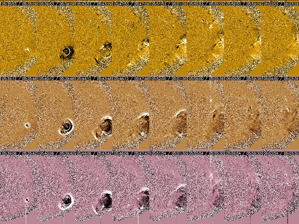
Figure 1. 24s running ratio AIA images of the 2010 June 13 EUV wave event, shown at four minute intervals. Shown from top to bottom are the Fe ix 171 Å, Fe xii 193 Å, and Fe xiv 211 Å filter channels, respectively. This event is characterized by a strong perturbation expanding outward in all directions that is positive the 193 and 211 Å bands and negative in the cooler 171 Å band. The high ratio cadence (24 s) allows for a much sharper view of the EUV wave front (outer component) and early on a clear separation between the EUV wave and trailing enhancement is observed (second and third frames). The inner component is identified as the CME by Patsourakos et al. (2010). The minimum and maximum color range for the ratio shown is 1 ± 0.02. Note: the different false coloring convention reflects the colors chosen by the AIA instrument team.
Download figure:
Standard image High-resolution imageAt this time, we were also fortunate that the separation of the STEREO spacecraft (Kaiser et al. 2008) had placed them at near right angles to the orbit of Earth. This meant that the EUV wave was observed almost directly on disk center by the EUVI instrument (Wuelser et al. 2004) on board the STEREO Ahead (STEREO-A) spacecraft, providing a completely complementary perspective and line-of-sight (LOS) projection of the EUV wave. At this time, the synoptic observing program for EUVI-A had only the 195 Å channel observing at a high cadence (2.5 minutes), but the general evolution and extent of the event was captured. EUVI-A 195 Å images of the event is shown in Figure 2, this time showing the running flux difference which better captures the EUV wave features when projected onto the solar disk.5 The images are processed as 2.5 minute running difference images and linearly scaled with ±5 DN s−1 min/max (the last image shows a 5 minute difference due to a data gap). From this perspective, the event exhibits the typical EUV wave characteristics (isotropic expansion, speed ranging from 250 to 350 km s−1), particularly for the eastward (red arrows) and westward propagation, which cannot be captured from the limb perspective of AIA. The northern component remains clearly visible until it encounters an active region, at which point the signal becomes obscured (more details in Section 4).
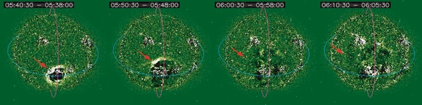
Figure 2. 2.5 minute running difference EUVI-A observations of the 2010 June 13 EUV wave shown at 10 minute intervals. From this STEREO-A perspective the eastward (red arrows) and westward propagation becomes clearly visible, features which cannot be captured from the limb perspective of AIA. For a scale perspective, the pink arc in each image represents a meridional arc of 1.2 R☉ centered above the eruption region, while the blue arc is the perpendicular great circle.
Download figure:
Standard image High-resolution image2.1. AIA Image Reduction Methods
Although AIA images are conveniently available only as already reduced Level 1 science products (Lemen et al. 2012), to extract the best signal for the EUV wave, the data is further processed for the following reasons. First, because EUV emission falls off sharply as a function distance from the solar limb (Flux∝n2e) the amount of photon noise increases the further one looks off of the limb for a fixed image exposure. Second, the photon S/N off of the limb is further reduced due to data compression algorithms that are applied onboard before each image is transmitted to the dedicated SDO ground-station. This process typically reduces the file-size by a factor of 7–10 (absolutely required for the experiment to function) and is designed to prioritize high-S/N features on the solar disk. This then presents a difficulty when attempting to extract the running flux evolution (already a derivative) of a signal that is typically no more than 5% over the background as the EUV wave propagates away from the eruption region. Fortunately, for the case of studying EUV waves, which are naturally large-scale, wide perturbations, the extreme high resolution of the AIA telescopes can harnessed to increase S/N by rebinning the 4096 × 4096 images down to a 512 × 512. The resulting binned image represents 64 pixel averages and increases the per-pixel S/N by a factor of eight. Additionally because the full 12 s cadence is not needed in the analysis, every other image is added together, further increasing the S/N ratio. Additionally for our quantitative flux plots in Section 4, we perform Gaussian convolution of each binned AIA image with a half width of σ = 0.03 R☉ (∼6 pixels in the rebinned images) before calculating the ratios in an attempt to draw out the large-scale properties of the event and further smooth out the effects of unrelated local variations and photon noise off of the limb.
3. NUMERICAL MODEL
In order to realistically simulate the conditions for the 2010 June 13 event we require an MHD model that accurately captures the thermodynamic state of the low-corona. To this end we employ the Lower Corona (LC) component of the Space Weather Modeling Framework (SWMF; Tóth et al. 2005). Details of the development and implementation of the LC component, which includes considerations relevant to resolving the thermodynamics of the low corona and transition region (e.g., radiative loss, field-aligned electron heat conduction, and empirical coronal heating in the energy equation), can be found in Downs et al. (2010). A first application of this model to the study of EUV waves can be found in Downs et al. (2011).
As in our previous work, we use a spherical (r, ϕ, θ) adaptive mesh refinement grid that is non-uniform in the radial direction. The r-coordinate is implemented to posses high resolution, transition region scales (min Δr < 210 km) at the r = 1 R☉ boundary of the model, and smoothly transition to logarithmic behavior at large radii. A minimum refinement of 64 × 128 × 64 is applied to the entire domain with an additional factor of two refinement below r = 1.7 R☉ for sub-polar co-latitudes (−65° < θ < 65°). A further factor of two refinement around the erupting active region, NOAA AR 11079, and nearby active regions, 11080 (adjacent), 11078 (farther west), and 11081 (north) is also applied. This gives maximum horizontal resolutions of ∼8.5 × 10³ km at the inner boundary around these active regions.
The initial magnetic field and boundary conditions are derived from a potential field source surface (PFSS; Altschuler et al. 1977) of synoptic radial magnetic field observations from the MDI instrument. Typically this involves constructing a synoptic map successive slices of observations around the central meridian during an entire solar rotation. However, for the 2010 June 13 event, ARs 11079, 11080, and 11081 began emerging shortly after their position had crossed the central meridian, and are more or less absent from a standard Carrington map for CR 2097. In order to represent these regions consistently in our model, we instead choose the MDI synoptic map created with a slice 45 deg west of the central meridian, which represents the use of observations ∼3.2 days after a standard Carrington map. To remove artifacts and correct for unobserved portions near the poles we smoothly transition to the polar corrected central meridian map provided by the MDI project for co-latitudes above 67° and below −67° over a width of ±5°. A comparison of a standard central meridian magnetogram and the custom magnetogram used in the simulation are shown in Figure 3. Utilizing measurements away from the central meridian does increase uncertainty in the radial field, but as is plainly visible, it is a necessary trade-off in order to include the near-eruption conditions around AR 11079.
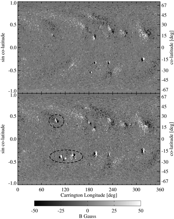
Figure 3. Comparison of the synoptic magnetograms discussed in Section 3 showing the results using meridional slices of observational data taken from either disk center (top) or 45° to solar west (bottom). The recently emerged active regions that require the 45° west slice are circled. The NOAA AR numbers are 11080, 11079, and 11078 (bottom circle, left to right) and 11081 is to the north (top circle).
Download figure:
Standard image High-resolution image3.1. Pre-event Conditions
The simulation itself consists of two stages. The initial step is designed to achieve an MHD equilibrium approximating the initial state of the pre-event corona, and the next step is to the evolve the eruption mechanism in time (described in Section 3.2). The 3D volume is first filled with a PFSS extrapolation of the input magnetogram calculated using the Finite Difference Iterative Potential-field Solver (FDIPS; Tóth et al. 2011) and a spherically symmetric Parker wind type solution. The system is then relaxed to a quasi-steady state by integrating the full thermodynamic MHD equations using the local time-stepping method (see Tóth et al. 2012; Cohen et al. 2008). By integrating with chromospheric boundary conditions and a suitable coronal heating model (Downs et al. 2011) thermodynamic balance over the transition region and magnetic topologies in the corona is achieved. It is important to emphasize here that by integrating the initial conditions to a steady MHD state, the resulting magnetic field configuration is no longer strictly potential and readily admits large-scale current sheets and regions of high plasma β (see Downs et al. 2010 for more details).
In order to directly compare the simulation results to observational data we must synthesize EUV observables from the simulation. The generation of synthetic EUV images involves using a description for plasma emissivity and detector/filter characterizations to generate a unit response function for each filter, fi(Te, ne), that depends strongly on electron temperature, Te, and weakly on electron density, ne. This function is then used to calculate the integrated emission along the LOS through the coronal plasma defined by each pixel and convert it to the predicted detector response:

where the n2e factor outside the filter specific fi is independent of temperature and reflects that the lines are formed collisionally. This method is based on that described by Mok et al. (2005) and Lionello et al. (2009), and a description of its use in the LC model can be found in Downs et al. (2010). The detector response curves used in generating synthetic AIA images in this work are shown in Figure 4, which gives pixel response in units of DN s−1 for a unit column emission measure (1026 cm−5) as a function of Te for each EUV channel of the AIA instrument. To be consistent with previous work, the spectral calculations are made using the CHIANTI 5 emission line analysis code (Landi et al. 2006), using the distribution's composite abundance file sun_coronal_ext.abund and composite ionization equilibrium file arnaud_raymond_ext.ioneq. Details on the calibration of AIA can be found in Boerner et al. (2012) and an analysis of the emission properties of the spectral lines observed by AIA as well as their relevance for various solar features can be found in O'Dwyer et al. (2010).

Figure 4. Temperature response of the seven standard EUV filters on the AIA instrument calculated with the CHIANTI 5 spectral synthesis code. The AIA 304, 171, 193, and 211 Å filters have similar response functions to their SOHO/EIT and STEREO/EUVI counterparts (193→195, 211→284) and possess a relatively high S/N due to the preponderance of coronal material emitting at their peak temperatures. AIA 94, 131, and 335 Å lines are intended primarily as probes for flare emission (they all have a high-temperature component), but all three also posses a cool coronal component as well.
Download figure:
Standard image High-resolution imageFigure 5 shows a pair of tri-color comparisons of AIA-EUV observations and those synthesized from the pre-event simulated conditions. Each tri-color image is an RGB composite of three different EUV filters (emission lines) where each filter is assigned a separate color channel. This serves to immediately highlight temperature-dependent density contrasts, and represents a useful analysis method, which is readily available due to the synchronized, high-cadence imaging of each AIA filter. The top panel displays a tri-color image composite of the Fe ix 171 Å (blue), Fe xii 193 Å (green), and Fe xiv 211 Å (red) filters, showing the temperature contrast for the three highest S/N filters of the AIA instrument.
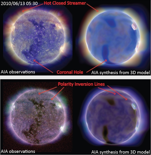
Figure 5. Tri-color intensity images of the pre-event state of the corona for observations (left) and emission synthesis from the LC model (right). As described in the text, each RGB color channel contains an intensity image of a particular AIA filter. Top row: AIA 171 (B), 193 (G), and 211 Å (R) showing the contrast of coronal plasma in the 0.8–2.0 MK range. The LC model adequately resolves the geometry and temperature contrast between open field coronal holes and hotter, closed streamer regions. Bottom row: AIA 193 (B), 335 (G), and 94 Å (R), which provides additional probe and comparison, emphasizing temperatures between 1.0 and 1.4 MK (red, blue) and those above 2.0 MK (green).
Download figure:
Standard image High-resolution imageAlthough the temperature peaks of the EUV filters are relatively broad, the tri-color images do well to highlight the temperature contrast between regions of closed field and open field, particularly on the solar limb. In the simulation the closed, QS, regions possess temperatures ranging from 1.2 ≲ Te ≲ 1.5 MK and appear reddish-green due to the heightened sensitivity in the 193 and 211 Å filters. On the other hand, open, coronal hole (CH) regions range from 0.9 ≲ Te ≲ 1.1 MK and appear predominantly blue due to their low temperature. The range of temperatures observed is due primarily to the feedback of the coronal heating terms and thermal conduction over the inherently complex 3D magnetic topology. For further comparison, the bottom panel shows and additional tri-color filter set: Fe xii 193 Å (blue), Fe xvi 335 Å (green), and Fe xiii 94 Å (red). The preponderance of the blue and red contribution is due to the sensitivity of the 193 and 94 Å filters to plasma in the 1.0 ≲ Te ≲ 1.4 MK range while for higher temperatures, the high-temperature component of the 335 line becomes relatively stronger.
The ability to capture both the general topological features of the corona and the relative contrast between filters of varying thermal response shows that the model does an adequate job of resolving the pre-event thermodynamic conditions of the corona on 2010 June 13. This is key, because any conclusions we draw on the physical nature of the event require that we accurately represent the conditions in which it propagates.
3.2. Eruption Model
The second stage of the simulation involves capturing the time-dependent dynamics of the eruption that generates the EUV wave transient. Because it is critically important that we compare the simulation results directly to AIA EUV data, we require an eruption model that is both applicable to realistic magnetic topologies and does not impose unrealistic temperature and density profiles at or near the source region. To this end we employ the bipolar charge-shearing eruption model first introduced by Roussev et al. (2007). We have previously used this eruption mechanism to study the properties of EUV waves with the LC model (Downs et al. 2011) and quickly summarize the properties here. In this model additional magnetic flux is added to the positive and negative polarities of the approximate bipole compromising AR 11079 in the form of two magnetic charges, +q, and −q (denoted q±), placed at locations  and
and  7 Mm below the surface, which are perpendicular to the polarity inversion line of the active region, and separated by an initial distance L0 = 15 Mm. A charge value of |q±| = 1.2 × 10¹¹ G km2 is applied, which corresponds approximately to an additional 58 G in magnitude added to each the existing polarity centers. This roughly doubles the total field strength of AR 11079 at the surface of the model.6 Starting from a relaxed MHD solution at t = t0, the charges are sheared in a quasi-steady manner at constant depth along the axis of the polarity inversion line at a linearly increasing speed that reaches v0 = 50 km s−1 at time t = 5 minutes (note that the coronal Alfvén speed is at or above 1000 km s−1 in the 50–100 Mm vicinity of the active region where the shearing takes place). The positive charge has a northward shearing component while the negative charge has a southward shearing component. The shearing motion continues at this speed until t = 30 minutes when the motion is ended. Magnetic flux density at the boundary is preserved by modifying the charge strength to account for the change in distance
  . The shear speed in the direction of the charge motion is also applied to the velocity boundary condition in the vicinity of each charge. Although this is clearly a simplification of the complexity of CME ignition mechanisms, the application of this scenario leads to the requisite onset of instability and a large-scale transient that exhibits the general properties of an EUV wave and CME traveling at 250–300 km s−1. We will explore the effect of alternative eruption mechanisms such as a superimposed unstable erupting flux-rope (e.g., Cohen et al. 2010; Lugaz et al. 2011) on the EUV wave transient in a future study.
4. EUV WAVE SIMULATION RESULTS
With our satisfactory pre-event conditions and eruption model in hand, we simulate the first 50 minutes of EUV wave transient. In order to best match to the evolution around 5:40 and beyond we elect to set the beginning of the shearing process at t0 = 5: 28 UT, about 7.5 minutes prior to the beginning of the flaring signal associated with the eruption (Ma et al. 2011). We focus our efforts in two main thrusts: first a characterization of the EUV transient observed by SDO/AIA involving the direct comparison of observations to the same observables synthesized from model data. And second, an in-depth analysis of the fundamental variables contained in the 3D simulation data, which provide insight to the physical mechanisms that create the multi-component features of EUV transient.
4.1. Comparison to EUV Observations
Figure 6 shows running ratio tri-color images of the EUV event between t =05:39 and 05:59 UT for observations (top) and the simulation (bottom) (see also the online animation associated with Figure 6). The time difference for the running ratio is chosen to be 48 s, which serves to slightly enhance and broaden the filter contrast in the images. Like the tri-color image for the pre-event conditions (Figure 5), each RGB color channel represents a separate AIA filter (171 (blue), 193 (green), and 211 Å (red)) only now the flux ratios for each band are scaled identically on a linear scale of (1 ± 0.035). This means that each particular offset in the relative phases or amplitudes of the perturbation for each channel will be spread across the RGB color plane. By nature this representation highlights anti-correlated ratio phases as having strong color components (e.g., negative ratios in 171 Å and positive ratios in 193 and 211 Å will appear yellow-red, while the opposite would appear bright blue). Correlated phases on the other hand (either all positive (white) or all negative (black)) will be confined to a mostly gray-scale range.

Figure 6. Tri-color running ratio images for the 2010 June 13 eruption using AIA observations (top) and image synthesis from the simulation (bottom). Shown at five, five, and ten minute intervals, respectively, starting from t = 05:39:38 UT, the three tri-color channels are AIA 171 (blue), 193 (green), and 211 Å (red) 48 s running ratios. The total intensity variation is identically scaled in each channel to a ratio of 1 ± 0.035. For a scale perspective, the pink arc in each image represents a meridional arc of 1.2 R☉ centered above the eruption region, while the blue arc is the perpendicular great circle.(An animation of this figure is available in the online journal.)
Download figure:
Standard image High-resolution imageFortuitously, due to the formation characteristics of EUV emission lines, this tri-color flux ratio method has direct relevance to separating temperature dominated perturbations from density perturbations. As illustrated in Equation (1), the bulk of the ne dependence lies outside of the filter specific response function, which implies that a pure density perturbation will have an identical phase in all filters (gray scale in the tri-color plot). A pure temperature perturbation on the other hand will produce a unique, filter dependent signal that depends on the local slope of fi at a particular temperature and can easily create anti-correlated phases between filters (picture sliding back and forth along the curves shown in Figure 4 for a fixed Te window). Of course, for plausible scenarios both a density and thermal perturbation will be present, but the relative contrast is still immediately apparent, due in part to the steep dependence of the filter response functions on temperature. For a more quantitative demonstration of this behavior, please refer to Appendix A.
The tri-color EUV images of the observations and simulations reveal two primary components that are important to discuss here: The outermost component, labeled in Figure 6, shows a nearly isotropic expanding hemispherical or "shell-like" feature that is seen as an enhancement in the 193 and 211 Å filters and as a relative flux decrease in the 171 Å filter (this is seen as a strong yellow-red color, red arrows in the tri-color images). As this component passes, the relative sign of the perturbation reverses in sign for all three filters and is seen as an enhancement in the cool 171 Å line (blue coloring, green arrows)). As discussed above, these color/phase signatures are highly suggestive of a heating and cooling cycle that occurs as the transient passes. This is not a new observational feature of EUV waves (e.g., Wills-Davey & Thompson 1999; Dai et al. 2010; Downs et al. 2011; Liu et al. 2010), but it is captured with extreme clarity due to the high-cadence multi-filter observing program of AIA. We identify this "hot-front" explicitly as the main EUV-wave component in the ensuing discussion.
Although somewhat difficult to see at later times, also present in the running ratio images is a secondary front that exhibits somewhat different properties than the outer EUV wave. Identified as the CME by Patsourakos et al. (2010) this front initially appears a strong hemispherical perturbation that is trailing the outer front (leftmost frame, 5:39:48 UT). As it expands, the transverse motion of this front is much slower and an extended cool dimming region is left in its wake. We identify this secondary component explicitly as the nonlinear or CME component in the ensuing discussion.
A full kinematic picture of the wave can be gleaned by constructing a time–distance representation of the EUV flux along a fixed set of points in space. Analogous to the time–distance diagrams described in Downs et al. (2011), we construct tri-color time–distance diagrams along an r = 1.2 R☉ arc that spans the western limb (we can examine a larger height than in the previous work because of the higher S/N ratio off of the limb for the binned AIA images, and the outer transient shows a higher relative amplitude at this distance). Shown in Figure 7 is the tri-color time–distance diagram for this event at 24 s sampling, which readily shows the speed and thermodynamic characteristics of the wave (outer "v" shape) as a continuous function of time (scale is now 1 ± 0.015)). Additionally the secondary enhancement that we identify as the "CME-component" is much more clear and appears as the inner "u" shape.7 Unique about this component is the fact that the tri-color perturbation color signal is noticeably different than the outer EUV front, first appearing light blue then light pink at later times, suggesting a significant density change that competes with the thermal changes. Most importantly we observe that this component slows enough that it remains confined to the latitudes between −45° and 0°, again a markedly different behavior than the outer EUV front, which propagates further and only mildly changes slope.
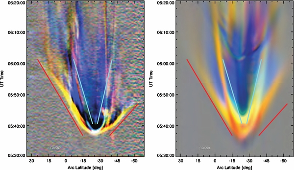
Figure 7. Tri-color time–distance diagrams made from observations (left) and model synthesis (right). The color channels are the same as in Figure 6 but they are now scaled to 1 ± 0.015 and show 24 s running ratios extracted along an r = 1.2 R☉ arc off of the solar limb (pink arc in Figure 6). This readily shows the speed (slope) and thermodynamic characteristics of the wave (outer "v" shape) as a function of time, which exhibits initial heating (yellow red) and subsequent cooling (blue) as it passes a fixed location. Additionally, the secondary enhancement due to the CME component appears as the inner "u" shape, which remains confined to the latitudes between −45° and 0°. Overlaid from left to right are lines with slopes of 400, 200, 150, and 600 km s−1, respectively, which show the approximate speed of the outer component (red lines) and inner component (cyan lines) in each direction. Please refer to Section 2.1 for a description of the image processing and spatial binning used.
Download figure:
Standard image High-resolution image4.1.1. Flux Comparisons
The main outer component of the EUV wave transient is further characterized by looking directly at the signal perturbation at various locations. Figure 8 shows flux versus time plots for AIA 171, 193, and 211 Å channels for four position angles along the r = 1.2 R☉ arc shown in Figure 6. Moving from north to south, panel (a) shows the flux evolution of the outer front far from the eruption site. The phase behavior that produces the color behavior of hot-front in Figures 6 and 7 is explicitly seen as anti-correlated slopes between the cool 171 Å filter and the hotter 193 and 211 Å filters, which is preserved in the presence of structures in a time-varying amplitude. Similar characteristics are observed in panel (b), taken at a latitude that is closer, but still relatively far from the eruption site. The overall amplitude here is higher, which is consistent with a pulse decreasing in amplitude as it propagates. Of note in both panels (a) and (b) is that all three of the filters share common inflection points (zero-crossings), which suggests that a common heating cooling mechanism is at play, rather than strong density modulation (would produce a common slope) or LOS effects involving multiple regions altering their temperatures. This type of behavior is consistent with a small amplitude adiabatic perturbation about the ambient plasma temperature (see Appendix A and the description of adiabatic warming observed by Schrijver et al. 2011). Comparing to the simulation for these locations, we see that the simulated transient does well to capture the anti-correlated phases and inflection point features in addition to recovering the overall width of the initial front and its arrival time (speed). However, the subsequent substructure that follows the initial front in observations is not particularly well produced, possibly a result of the difficulty of resolving the fine-scale structures of the ambient corona with a global MHD model.

Figure 8. Flux vs. time plots for the AIA 171, 193, and 211 Å channels comparing the observations (top traces) to model synthesis (bottom traces). The panels show fluxes extracted at four position angles along a r = 1.2 R☉ off of the solar limb (pink arc in Figure 6). Arc positions (a), (b), and (c) are located in the path of the northern front, while arc (d) is located in the path of the southern front. Refer to the x-axis of Figure 7 for a sense of where these latitude positions lie with respect to the front.
Download figure:
Standard image High-resolution imageCloser to the eruption (panel c) the oscillation is present but modulated in the AIA observations. The 171 Å flux does not share the same inflection point as 193 or 211 Å and all of the three flux ratios do not return to zero. This suggests that we are observing a mix of linear and nonlinear features due to the proximity to the eruption site and subsequent passage of the secondary front. Lastly, the location examined in panel (d) is in the path of the southern front and very near to the observed boundary between the closed field streamer and southern coronal hole. Both model and observations show the same qualitative phase relationship but the observed front is sharper (less broad) here than in the northern front and in the simulated flux ratio, and also passes about five minutes earlier than the simulation. Both effects are likely due to the increased propagation speed of the southern front with respect to the northern front, which is not resolved in the model. We posit that this is due to the presence of relatively stronger field (faster magneto-sonic speed) in this region of the corona than is resolved in the model. Polar regions (particularly open/closed boundaries) are always more difficult to reproduce in magnetic extrapolations than equatorial regions directly because the LOS component of the observed magnetic field measured at the surface gets farther away from radial as we near the poles. At any rate, the correlation of the front with the fast magnetosonic sound speed is investigated in Section 4.2.
The inner, secondary component of the event is more difficult to pick out in running ratio observations due its slow transverse speed, so we instead turn to examining the base ratio for EUV flux relative to 05:30:02 UT. Unlike the running flux ratios, base processing highlights the zero-order nonlinear changes that occur in the coronal plasma. Zero-order change is, of course, expected to be introduced by the CME eruption itself which often causes mass depletion and reduced EUV emission (coronal dimming, see Aschwanden 2009 for example). In Figure 9, we show the base ratio flux evolution for the event at four times along the entire r = 1.2 R☉ arc (note the reversal of time-space roles with respect to Figure 8, as now arc latitude is the continuous variable). The strong nonlinear (as high as 1.5 in 171 Å) evolution of this component creates the large peaks at nearly fixed latitudes along the arc, marking the edges of the volume carved out by the eruption. This forms the "well-shaped" signal (deep minimum, side maximums) spanning approximately −45° to 0° latitude in Figure 9. The model does well to reproduce the size of the secondary EUV perturbation caused by the CME but not the deep dimming (mass depletion) and precise thermodynamic signal (too much enhancement in the 211 Å channel).
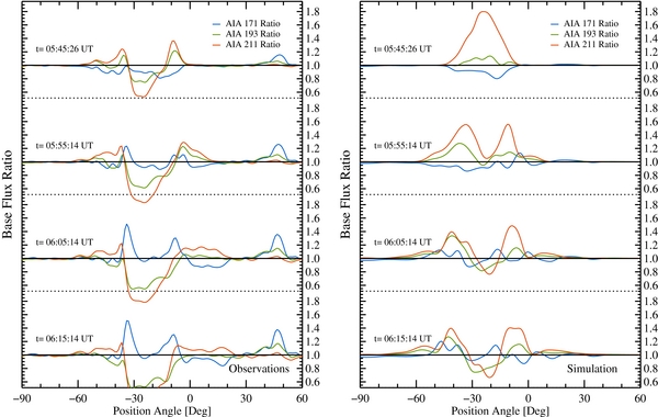
Figure 9. Base flux ratio measured along the r = 1.2 R☉ arc at t = 05:45:26, 05:55:14, 06:05:14, and 06:15:14 UT for observations (left) and the simulation (right). The base time chosen for the flux ratio is 05:30:02 UT, and the trace for each filter is interpolated to a common time. The secondary EUV component is identified as the "well-shaped" signal (deep minimum, side maximums) spanning approximately −45° to 0° latitude. The EUV wave is barely perceptible in this representation ahead of the CME flanks due to its low absolute amplitude (≲ 5%). The signal at +45° latitude is caused by the rising of an unrelated prominence off of the northwest limb.
Download figure:
Standard image High-resolution imageThrough this analysis, we demonstrate that many of the important observational characteristics of the EUV transient are captured by the simulation. This includes:
- 1.The extent and speed of the outer EUV wave in the northern direction.
- 2.The approximate width of the initial pulse.
- 3.The anti-correlated filter phases that indicate heating/cooling within the front.
- 4.The kinematics and physical extent of the secondary EUV component.
4.2. Analysis of the 3D Data
In order for the coupled observation and modeling analysis to succeed it is critically important that the simulated EUV wave reproduce the basic characteristics of the observations. However, matching these observations alone do constrain the physical mechanisms behind the perturbation signal. In order to address this we turn to analysis of the temporal evolution of the full 3D set of eight MHD variables namely: density, ρ, vector velocity,  , vector magnetic field,
  , and electron temperature, Te. Note: from hereafter simulation time references will be with respect to the beginning of the simulation, t0 = 05:28 UT.
First off it is important to correlate the main time-dependent components discussed in the EUV analysis to variables from the simulation data directly (density, temperature, velocity, and magnetic field). From our experience in Downs et al. (2011) and this work, we find that the perturbations in the density (ne or n2e) best correlate to the EUV perturbation in the synthetic images. Although the temperature plays an important role in determining where a parcel of plasma lies in a given filters thermal response curve (Figure 4), it is the outer n2e dependence that is guaranteed to modulate the signal regardless of temperature. In order to isolate the time-evolving transient over the background, we take snapshots of the 3D simulation every 48 s and calculate the running ratio of density at all points in space, and use this variable in the discussion below.
4.2.1. Correlation to the Fast-mode Speed
The next order of business is to examine the applicability of various EUV wave mechanisms to the simulation results, beginning with the most popular candidate: EUV wave as fast-mode waves. Fortuitously, the ambient magnetic field and position of the erupting active region provide excellent conditions to test the correlation of the EUV perturbation with the local fast-mode wave propagation speed, cf, in the corona. The fast-mode speed varies depending on propagation angle with respect to magnetic field, so we use the maximum value,  , where
  and
and  are the Alfvén and sound speeds of the plasma, respectively. Shown in Figure 10 are color contours of cmaxf for both the SDO and STEREO-A perspectives at twelve minute intervals. The EUV wave evolution is highlighted in each frame by overlaying line contours of positive values of running density ratio, which helps to isolate the outer front in particular.
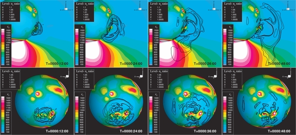
Figure 10. Correlation of the density enhancement (black contour lines) with the perpendicular fast-magnetosonic speed (color contours) from the AIA perspective (top) and the STEREO-A/EUVI perspective (bottom). Both perspectives show cf and the density ratio on a sphere of r = 1.1 R☉, and also the meridional plane intersecting AR 11079 for the top AIA perspective. The outer evolution of the black contour lines track the global EUV perturbation, which shows a clear alteration in shape as it encounters the southern coronal hole. Also visible from the STEREO-A perspective is the steepening and slowing down of the eastern front as it encounters the region of smaller cf as well as the loss of signal as it encounters the northern active region.
Download figure:
Standard image High-resolution imageStarting with the SDO/AIA perspective (top row), we see that in the northern direction of propagation, away from the high localized field of the active region, cf is fairly uniform for a large volume and confined to a narrow range of ∼200–350 km s−1 (200 km s−1 represents a floor set by cs for million degree plasma, which is independent of  ). However, in the southern direction, the presence of a nearby coronal hole (lower ne and Te, higher
  ) enforces that cf begins increasing rapidly over a short distance when the coronal hole boundary is reached. If the transient is indeed a pure fast-mode wave this would imply significantly different characteristics between the north and south fronts of the wave, which is precisely what is observed. As the northern portion of the front propagates, it retains a roughly hemispherical shape, which is expected for uniform propagation speeds. To the south however, as the front begins to encounter the large gradient in cf, its collective shape appears to both speed up and shear/refract to a broader north south alignment, one far removed from the original hemispherical shape. In wave terms this collective behavior would be expected, as each individual wave packet will (1) travel at slightly different speed, altering the location where the enhancements line up, hence shape of the front, (2) undergo broadening (due to speed increase) and (3) experience a significantly increased reflection probability (due to speed gradient).
Now turning to the STEREO-A/EUVI perspective (Figure 10, bottom row) we observe an analogous situation play out over the solar disk. Initially (t < 25 minutes), the eastern (left), northern, and western propagation of the outer front is through regions with a roughly comparable value of cf. At this time the roughly circular nature of the front is preserved (a circle is the projection of a hemisphere on the disk). At later times, two interesting features are observed: First, in the eastern direction, the transient encounters a large region with a relatively smaller value of cf (extended QS) and exhibits both a slowing down and steepening in relative magnitude. This resembles the behavior of wave-packets steepening as they begin piling up when forced to slow down due to decreased propagation speed. Second, the transient eventually encounters the influence of the AR 11081 and adjacent high-field region in the north, which provides a relatively sharp increase in cf. As it encounters AR 11081, the northern transient begins to broaden and distort the originally circular shape, eventually losing visibility at this scaling level, characteristics that again support the wave hypothesis. The applicability of this analysis is confirmed by comparing the STEREO-A/EUVI 195 Å observations directly to synthesized images, which is done in Figure 11. The eastern propagation of the front in observations is reproduced by the model and is coincident with the density perturbation shown in Figure 10. Additionally, the relative absence of the transient signal above the northern AR is reproduced.
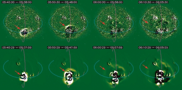
Figure 11. Comparison of EUVI-A observations (top) to EUVI-A image synthesis (bottom) of the EUV wave transient in the simulation. The running difference processing is the same as in Figure 2, and the red arrows tracking the eastern propagation of the transient are at identical locations for each column. The outer EUV front in the synthesized data appears at the same locations as the perturbed density contours in Figure 10 and tracks the shape of the observed front quite well in the eastern, northern, and western directions.
Download figure:
Standard image High-resolution image4.2.2. Phase Analysis
In order to gain further insight into the wave nature of the extended front we turn to considering the linearized MHD equations in a uniform medium. There are numerous ways for expressing the characteristic waves in MHD, and for the purpose of this discussion we use the form presented in Lectures 19–24 of Schnack (2009) and refer the reader there for complete details. Assuming a uniform magnetized medium with no flow, first decompose the system into a constant background ( ) plus linear perturbations about the background (
 ). This representation can be used to linearize the ideal MHD equations by substituting this form and then canceling of derivatives of constant quantities and terms involving more than one power of perturbed terms. Now, given a small linear displacement of a fluid element about its equilibrium position,
  , an evolutionary equation for
  can be directly formulated:

Standard solutions for the characteristic eigenvalues and eigenfunctions can be determined by substituting a plane wave solution, ![${\bm \xi }({\bm r}, t) = {\bm \xi }_0 \exp [{i({\bm k} \cdot {{\bm r} + \omega t})}]$](https://content.cld.iop.org/journals/0004-637X/750/2/134/revision1/apj425465ieqn15.gif) , where
, where  is the direction of propagation, which leads directly to the separation of the three MHD wave modes: the fast and slow magnetosonic waves, and Alfvén waves. Additionally, any linear displacement
  can be represented as a linear superposition of the eigenvectors of each of the three modes,
  . What is most pertinent to take from this discussion is the relative phases of the velocity and density perturbation, respectively:

Since the velocity perturbation is a vector quantity it is difficult to analyze because its projections depend on a choice of coordinate system, we go further and examine the phase of its divergence, a scalar quantity:

Because of the additional derivative,  is 270° out of phase of ρ1, which makes for a unique signature to look at when identifying components in the simulation that exhibit linear, compressible, wavelike behavior.
In order to apply the above illustration to variables calculated in the simulation, we make the identification of ρ1 → ne running ratio, and  running difference. The running method is chosen because it isolates the short term low amplitude transient from long term variations. We should note here that this calculation technically adds an effective derivative and is noisier, however this acceptable because the phase relationship will still be preserved by definition.
The top panels of Figure 12 show a comparison of the running difference of  (color contour) and running ratio of ne (lines) for t = 28 and 44 minutes with a 48 sec ratio/difference. Examining the outer component of both the southern and northern fronts at t = 28 minutes, we observe the characteristic signature of a 270° phase relationship, i.e., a positive to negative sign reversal for
  at the peak the of ne enhancement. 16 minutes later this feature is still quite conspicuous in the north where the fast-mode speed is still relatively low and uniform. It becomes distorted in the south due to the passage into the coronal hole region, but the phase relationship remains quite clear. This reinforces and is consistent with the wavelike behavior discussed in the previous section (also see Figures 10 and 11).

Figure 12. Snapshots of the simulation at t = 28: 00 minutes (left) and t = 44: 00 minutes (right) for three parameters on the meridional plane intersecting AR 11079 and sphere of r = 1.1 R☉. The identical black contours in each panel represent positive values of running density ratio (perturbed ρ1). Top row: the relative phases of the perturbed density and velocity divergence,  (color), showing a 270° phase offset in the outer front. This can be identified by looking at the location of the positive to negative inflection point of
  (pink→yellow→blue shows +→0 → −), which resides precisely along the peak of the positive density perturbation. Middle row: the magnitude of the fluid velocity,
  , showing the bulk motion of the CME as it propagates outward. Large, nonlinear changes in
  are localized to the region directly above the eruption and are mostly absent from the outer front that exhibits the EUV wave behavior. Bottom row: the running 48 s difference of the current parameter α for both times. The strong positive and negative values of this parameter define the "expanding current shell" which is directly correlated with the bulk velocity enhancement in the middle row, and not the outer EUV wave front, particularly in the transverse directions.
Download figure:
Standard image High-resolution imageA necessary step in this analysis is to now separate the fast-mode wave component from that of the nonlinear evolution of the CME eruption itself. We illustrate this in two ways, first by examining the bulk velocity of the eruption and then by looking at the currents that are produced, both of which help localize the CME component of the EUV perturbation. The middle panels of Figure 12 show the absolute value of flow velocity for t = 28 and 44 minutes. Immediately apparent is the relatively central locality of the bulk velocity of the CME. The outer compression fronts identified in the top panels show little absolute velocity difference from their surroundings, while the central core of the CME itself is accelerated to a few hundred kilometers per second and is flowing outwards.
Further evidence supporting a separation between nonlinear CME evolution and the EUV wave can be found in the MHD currents formed during the eruption. The bottom panels of Figure 12 show running difference values of the parameter  =
=  for the same times and cadence as the top panels. A critical parameter supporting the current shell hypothesis discussed in a simulation by Delannée et al. (2008), α is a scalar quantity that illustrates where field-aligned currents are strong relative to the local magnetic field. Indicative of nonlinearly evolving magnetic structures, this parameter traces regions of expanding and contracting systems of magnetic flux within the CME eruption. Note that for the purely linear displacement described above, α is identically zero because
  and
and  and
and  are mutually orthogonal for the slow and fast eigenmodes. Comparing the three rows of panels in Figure 12 we see that the α perturbation is mainly localized to the eruption region and strongly correlated with the bulk velocity of the CME, and not strongly associated with the outer front of density perturbation. This allows us to identify the inner component of nonlinear evolution as the manifestation of the often discussed non-wave components theorized to explain EUV waves. This current evolution resembles the "field line stretching" model discussed by Chen et al. (2011), the "current shell" model of Delannée et al. (2008), and the "non-wave" components modeled by Cohen et al. (2009) and Downs et al. (2011). Of course, because static MHD currents are admitted in the pre-event equilibrium (
 ), we expect a small, orientation dependent signal in α from a linear fast-mode wave. However, the total absolute change in α away from the bulk velocity enhancements is over an order of magnitude less than the 0.5 value used to visualize the outer shell in (Delannée et al. 2008) (though these absolute values depend on the eruption model and numerical resolution).
5. DISCUSSION AND CONCLUSIONS
In this work we explore the physical underpinnings of the 2010 June 13 EUV wave by characterizing the event within a 3D time-dependent thermodynamic MHD model of the global corona. The crux of this analysis relies of the assertion that the transient simulated in the model provides a realistic accounting of the true event that is observed. This connection is established by the forward modeling of observational data (EUV images), the results of which can be used for a direct comparison to observations. This is done on a one-to-one basis qualitatively for the pre-event conditions (Section 3.1 and Figure 5) and quantitatively for the time-dependent signature of the EUV transient (Section 4.1 and Figures 6–9 and 11). With this important link in place, we find strong evidence in the simulation that the outer, propagating component of the perturbation exhibits the unequivocal behavior of a fast-mode wave. We also find that this component becomes decoupled from the evolving structures associated with the CME that are also visible (Section 4.2 and Figures 10 and 12). This provides strong support for the fast-mode wave interpretation of EUV waves (Gopalswamy et al. 2009; Patsourakos et al. 2009; Patsourakos & Vourlidas 2009) and models combining both wave and non-wave components, where the fast-mode wave is primarily responsible for the outer propagating front (Cohen et al. 2009; Downs et al. 2011). Before going on, the implications of these results for purely non-wave explanations for EUV waves are discussed below.
5.1. Relevance to Proposed "Non-wave" Mechanisms
Field line stretching model. The idea of an EUV wave event possessing both a fast-mode wave and trailing nonlinear component is not new. In fact, the "field-line stretching" model originally proposed by Chen et al. (2002) and subsequently studied by Chen et al. (2005, 2011; among others) predicts exactly this situation. The key distinction however is in the physical mechanism responsible for the EUV emission in the globally propagating front. In an effort to unify coronal signatures with Moreton waves (fast-mode waves traveling at high speeds in the chromosphere) the field-line stretching model proposes that a coronal Moreton wave (fast-mode wave) is launched during the eruption and propagates freely in all directions under coronal conditions. The EUV signature however is not produced by the coronal Moreton wave (argued to be relatively undetectable) and instead it is the subsequent expansion of the CME and surrounding of the arcade that creates this signature. The enhanced emission produced by the "stretching" of field pulled along with the CME and its subsequent compression on the surrounding regions, this behavior was also observed and studied in our previous study (Downs et al. 2011). For the 2010 June 13 event we find both strong evidence for both components as well, and in a semantic sense confirm their scenario. However, our analysis confirms that outer fast-magnetosonic wave component is not only observable but is in fact clearly responsible for the ubiquitous features of EUV waves, (nearly isotropic at onset, large transverse propagation distances, modulation due to local fast-mode magnetosonic speed, decoupling from the CME source region). This is a significant physical distinction.
Current shell model. Briefly mentioned in the analysis of the current parameter, α, in Section 4.2 and Figure 12, is another non-wave theory for the transient EUV signature of the outer front: the "current shell" model proposed by Delannée et al. (2008) and subsequently explored in Delannée (2009) and Schrijver et al. (2011). This scenario features a erupting flux rope that forms an expanding shell or layer of localized MHD currents as it impinges on the surrounding field in the corona. This represents the nonlinear contribution of the changing magnetic field in the induction equation. These currents are then thought to generate an observable EUV transient by heating the coronal plasma as they dissipate. Indeed we can identify this phenomena taking place in both the EUV observations and in the MHD simulation of the eruption. However, it is the location of these currents that are problematic for this model to apply to this event. As shown in Figure 12, the current shell is confined (as expected) to the region of the CME itself and does not extend strongly into the outer front where the outer EUV wave signal is produced. Here the time-dependent signal in α is more than an order of magnitude weaker, and lacks coherence with the outer front (compare the top and bottom panels of Figure 12). Furthermore the heating and cooling observed in the outer front is completely consistent with that of a compressible wave, whose nature is confirmed by the relative phase analysis.
Although we demonstrate that an expanding current shell was not required to reproduce the observable characteristics of the outer EUV wave front in this case, it is important to note that we use a significantly different driving mechanism to initiate the eruption than the flux-rope formed in the zero-β simulations presented by Delannée et al. (2008) and Schrijver et al. (2011), and recognize that the driver plays a key role in determining the EUV transient signal (see discussion below). Self consistent thermodynamic simulations comparing such factors are left for future work.
Reconnection front. Another explanation for the characteristic signature of EUV transients is the "reconnection-front" model proposed by (Attrill et al. 2007a) and argued observationally by Attrill et al. (2007b) and Dai et al. (2010). In this scenario, the EUV wave signature is generated by successive reconnection events of favorably oriented field with the expanding field of the CME eruption. These successive reconnection events dissipate magnetic energy, conducting thermal energy upwards along connected magnetic field lines, ultimately creating the collective front that is observed. As with our previous work (Downs et al. 2011) we do not find evidence for these mechanisms playing a role outside of the immediate vicinity of the eruption region (which is complicated by all the other nonlinear terms). A thermal conduction front due to reconnection would necessarily need to be correlated to the CME evolution (not the case for the outer front), and would not be directly correlated to fast-magnetosonic speed (contrary to what is observed). Of course, the numerical limitations of modeling the global corona via our thermodynamic MHD model imply that resolving the details of small-scale low-lying mixed polarities and their associated reconnections over the entire QS cannot be adequately addressed here. However, we do show that such a scenario is not required to reproduce the observable signal of the EUV wave front in the model, an important distinction.
Slow-mode mechanisms. The last set of "non-wave" explanations for EUV waves that we briefly address are the various works that explore the applicability of slow-mode mechanisms. Although the slow-mode is indeed a wave characteristic of the MHD equations, due to the unusual nature of slow-mode waves EUV wave mechanisms employing them typically invoke nonlinear slow-mode processes, such as a coherent soliton pulse (Wills-Davey et al. 2007) or the steepening of a slow-mode shock, such as the one described in Wang et al. (2009). Although we do not address any particular slow-mode theory directly here, we do not find strong evidence for slow-mode mechanisms contributing to the extended outer front. First off, in the transverse directions (north, south, east, west) the outer front does not develop characteristics indicative of a steep MHD shock, the pulse remains in a linear regime (sub 5%) while decaying and does not incur large enough flow velocities (Figure 12, middle row) to exceed the speeds of the local eigenmodes. (Of course, the slow-mode shock simulated in the ideal conditions simulated in Wang et al. 2009 could explain the EUV signal we identify as the flanks of the CME).
Turning to phase speeds directly, we note that in the strong field limit, the fast-mode speed does not depend strongly on the orientation angle, θ, between the propagation direction and local direction of the magnetic field:  . On the other hand the slow-mode speed, cslow, varies significantly with orientation in the strong field limit: cslow ≈ cscos θ, and goes to zero for perpendicular propagation. In our simulation, a drastic change in the front speed that depends on the orientation of
  is not observed at any location along the outer propagating front. From the AIA perspective shown in Figures 10 and 12 the outward propagating front encounters parallel field, while the northern and southern components encounter initially perpendicular field, and all three directions show a similar behavior. The phase relationship identifies a compressible wave for this front (both fast- and slow-mode waves are compressible), but a slow-mode wave would not be able to simultaneously satisfy the isotropic nature that is observed.
5.2. A Unified Wave/Non-wave Picture
In our analysis of this event Section 4 we find strong evidence supporting the identification of the outer EUV transient observed by AIA and EUVI-A as a fast-mode MHD wave. This should not, however, marginalize the role that the nonlinear evolution of the eruption plays in the overall set of EUV signatures that are observed. If say, for arguments sake, that this specific eruption proceeded twice as fast, released twice as much energy, or occurred in a corona with twice the ambient magnetic field strength, then the resulting EUV signature (all fronts) would most definitely be altered in some way (in fact, we explicitly explore this in Downs et al. 2011). These mock scenarios are relevant to reality in the sense that the conditions of the corona are never the same for any two events and, as a result, it is not guaranteed to always be the case that a particular scenario will be universally applicable. This implies that the relative contribution of the outer wave component and inner CME component will likely depend highly on the specific conditions and eruption mechanism for every event. Clearly if the erupting flux system possesses a significant transverse extent in the low corona and the speed of this process approaches that of the fast-mode wave front, then the two features will become difficult to distinguish (e.g., Run A in Downs et al. 2011). All in all, this reinforces the need for a broad perspective and when considering possible EUV wave mechanisms and that considerations of specific, and realistic conditions for each event are extremely important. In the event studied here we are able to clearly identify and separate the fast-mode wave responsible for the EUV wave from the strong currents and CME evolution that also provide an EUV signal, but this may not always be the case for future events that will be captured by AIA or other future observing facilities.
Along these lines we promote a combined wave/non-wave picture of EUV wave transients, one where the outer EUV front is initially driven by the solar eruption, but later becomes a freely propagating fast-magnetosonic wave. The unique, event specific evolution of the solar eruption however will continue to produce some observable features in the EUV (this is the same scenario discussed in Zhukov & Auchère 2004; Cohen et al. 2009; Patsourakos et al. 2009; Patsourakos & Vourlidas 2009; Downs et al. 2011; Grechnev et al. 2011a). Surely a fast-mode wave will exist on some level when the corona is perturbed (perturbed strongly in the case of CMEs) because fast-magnetosonic waves are a primary means of information transport across field lines in a magnetized plasma. Additionally, fast-mode waves by their very nature conveniently satisfy the global, perpendicularly propagating nature of observed EUV wave transients, without relying on a particular set of constraints on the ambient conditions. This is quite compelling as it relaxes the need for the various "non-wave" mechanisms to require the CME/coronal arcade to posses physical extents of a solar radii or more relatively close to the surface, a significant physical difficulty for the basic models of CMEs. But the fast-mode wave cannot fulfill all observational requirements on its own! Some events, such as the slowest reported waves (50–200 km s−1), and features such as extended dimming regions and persistent brightenings simply cannot be described by fast-mode waves. Here, the non-wave, nonlinear evolution of the event itself saves the day by bringing a slew of nonlinear mechanisms to the table. With this framework, we theorize that many of the slowest reported EUV waves (Wills-Davey et al. 2007; Warmuth & Mann 2011) were in fact measuring the secondary component of a weak eruption where the initial fast-mode wave was not detectable given pre-AIA instrument and cadence limitations.
Of course, not all aspects of EUV waves can be addressed in a single simulation. Of particular interest is the precise way in which the flare/CME driving occurs in the low corona, which is relevant both to our physical understanding and classification of EUV waves (Warmuth & Mann 2011). Recent work by Grechnev et al. (2011a, 2011b) and Afanasyev & Uralov (2011) suggests that the initial expansion of the CME acts as an impulsive piston, launching a weak fast-mode shock wave ahead of the evolving CME structures. Grechnev et al. (2011a) in particular take great care to make a distinction between this case and driving of the wave pulse by the flanks of the CME until lateral expansion ends (e.g., Veronig et al. 2010). However, due to the relative simplicity of the eruption model and the lack of a realistic MHD description of fast reconnection (which limits the rate at which the CME is impulsively accelerated early on) we cannot confidently discriminate between these scenarios in this case (compare the early width of the EUV signature between the model and observations in Figure 7). In principle, this issue can be addressed through an in-depth study of the early evolution of the eruption mechanism and by leveraging the rich time–distance signatures present in AIA observations, which we leave to future work.
As far as a flare pressure pulse as a possible driver for the EUV wave, we note that at no point in the simulation are flare like temperatures achieved (Te ≲ 6 MK during the run). This limits our ability to explore a flare-like pressure pulse in a realistic fashion, but we do not require these temperatures to produce the observable EUV wave features (see review by Zhukov (2011) and references therein for a further discussion on this topic).
Ultimately the strong implications towards EUV mechanisms discussed here are directly borne out of the fact that the AIA instrument and its high-cadence, high-resolution synoptic observing program offers a new source of unprecedentedly detailed observations with which to study EUV waves. Without a source of strong observational constraint, particularly for events that never occur the exact same way twice, it becomes exceedingly difficult to constrain the theoretical models. Models that all too often are lacking with respect to a rigorous prescription of the mechanisms behind the observable features. To this end we attempt to unify the two, employing a state-of-the-art model and an analysis of cutting edge observations. We model an EUV transient without assuming a priori a particular theory or explanation, and instead it is the plausible connection to observations that gives credence to the physical mechanisms identified in the results—results which, we hope, help to eliminate the suspension of disbelief that is sometimes required for physical interpretations when either the model or observations are incomplete.
The authors thank the anonymous referee for their useful comments, which helped improve the manuscript. This work is primarily supported under the NASA Earth and Space Science Fellowship (NESSF) Program NASA NESSF08-Helio08F-0007 as well as grants: NSF ATM-0639335 (CAREER), NASA NNX08AQ16G (LWS), and NSF ATM-0120950. Preliminary computations were performed on the computing cluster at the Institute for Astronomy Advanced Technology Research Center. Final simulations were conducted on resources provided by the Hawaii Open Supercomputing Center.
The SECCHI data used here were produced by an international consortium of the Naval Research Laboratory (USA), Lockheed Martin Solar and Astrophysics Lab (USA), NASA Goddard Space Flight Center (USA), Rutherford Appleton Laboratory (UK), University of Birmingham (UK), Max-Planck-Institut for Solar System Research (Germany), Centre Spatiale de Liège (Belgium), Institut d'Optique Théorique et Appliquée (France), and Institut d'Astrophysique Spatiale (France). This work was supported by NASA.
SDO/AIA data products are courtesy of NASA/SDO and the AIA, EVE, and HMI science teams.
APPENDIX: INTERPRETING THE TRI-COLOR RATIO SIGNAL
In Section 4.1, we qualitatively discuss the relationship between plasma heating/cooling and the colored signal produced in the tri-color running ratio composite images of the EUV transient. The interpretation of the signal in Figures 6 and 7 can be aided by examining this response for an ideal system. Consider a unit parcel of coronal material at a fixed electron temperature and density T0 and n0. In this case, one can calculate the unit emissivity, fi, 0(T0, n0), for a particular EUV filter in the same manner as described in Section 3.1. Now consider imposing a small perturbation on T0 and n0 and again computing the emissivity for the perturbed state to obtain fi, 1(T0 + ΔT, n0 + Δn). The ratio Ri = (1 + Δn/n0)2fi, 1/fi, 0 then defines the input of a particular filters flux ratio to its corresponding color channel in the tri-color images.
Given that fi(Te, ne) is a slowly varying function of density, we choose a fixed value of n0 = 1 × 108 cm−3, and explore the dependence of Ri(T0, ΔT, Δn) as a function of initial temperature and the input perturbation. Figure 13 shows the result for a set of three perturbations for both positive (top row) and negative values (bottom row). Choosing ΔT = ±0.003T0 = 0.3% for all frames, we show the resulting tri-color signal for the case of a zero (left), adiabatic (middle), and twice adiabatic (right) density perturbation. The line plots in each frame of Figure 13 reflect the ratio, Ri(T0, ΔT, Δn), for a given filter (171 Å blue, 193 Å green, 211 Å orange) while the colored background shows the combined tri-color signal as it varies with T0. The color ranges, scaled identically to Figure 7, saturate at 1 ± 0.015. The adiabatic perturbations are calculated by assuming T/ργ − 1 is constant for an adiabatic process (zero heat transfer), which gives 1 + Δn/n = (1 + ΔT/T)1/(γ − 1), where γ = 5/3. We choose the Δn range to reflect the fact that nonlinear processes in the corona (bulk flow, MHD currents, thermal conduction) that might contribute to the transient may not always create adiabatic perturbations.
Figure 13. Tri-color signal as a function of temperature for three separate perturbations of a unit parcel of coronal material. The temperature perturbation is ΔT = ±0.3% for all three frames with positive values in the top row and negative values in the bottom row. From left to right, the density perturbation is zero, adiabatic, and twice adiabatic. The line plots in each frame reflect the ratio, Ri(T0, ΔT, Δn), for a given filter (171 Å blue, 193 Å green, 211 Å orange) while the colored background shows the combined tri-color signal as it varies with T0. The color ranges are scaled identically to Figure 7 and saturate at 1 ± 0.015.
Download figure:
Standard image High-resolution image
As can be seen following the sequence from left to right, the ΔT perturbation creates the relative shapes of the ratio signals while the Δn perturbation serves as an offset to all three.8 The preponderance of the yellow to orange tri-color signal in the 1–1.6 MK QS temperature range for all three scenarios confirms that a small positive perturbation can reproduce the signal observed in the outer EUV front (Figure 7), and equally reproduce the negative (blue) signal as the front passes. Excess heating or cooling, outside of what would be expected for a compressional wave perturbation, is clearly not required (though not ruled out).
Of course, LOS projections through multi-temperature plasma undergoing a large-scale perturbation will complicate the signal. However, due to the apparent sensitivity of the tri-color ratios to hone in on a specific temperature given a known perturbation, this does suggest, given the excellent cadence and data fidelity of AIA, that a future study could leverage this technique to independently constrain temperatures in regions of the corona–a so called temperature seismology' technique. While not exhaustive by any means, this provides a relatable metric to interpret the complex tri-color signal in the observations and simulation results presented here.
Footnotes
- 3
For clarity in the ensuing discussion, we choose to adopt the Cohen et al. (2009) convention of referring to these phenomena as "EUV waves," a general term, one which naturally includes observations from the modern generation of EUV imagers, rather than the conventional term "EIT waves"; a specific reference to the EIT instrument.
- 4
In reference to an idiosyncratic convention of the study of EUV waves, we wish to make clear that the adopted terminology "EUV wave" refers to the appearance of the observed phenomena itself, and does not imply judgment that this is necessary a physical wave.
- 5
For a more in-depth discussion on the relative advantages/uses of flux differencing or flux ratios and running and base methods, please refer to Downs et al. (2011).
- 6
Note that PFSS extrapolation to the resolution of the MHD model smooths out the highest field strengths seen in the synoptic magnetogram observations (Figure 3).
- 7
The synthetic image in Figure 7 shows a secondary transient "u" feature at 6:08 UT, this is an unfortunate artifact due to halting of the shearing process (50 → 0 km s−1) and is not physically meaningful.
- 8
A purely isothermal perturbation (ΔT = 0) would appear as nearly gray scale in this representation. This is due to the fact that the relative variation of fi(Te, ne) with density is more than an order of magnitude less than its variation with temperature for comparable small values of ΔT and Δn.