

Abstract
In general, superconducting tokamaks require low loop voltage current start-up for the safety purpose of their poloidal field coils. The loop voltage inside the vacuum vessel of Steady State Superconducting Tokamak (SST-1) is low in nature since its central solenoid is located outside the cryostat. The low loop voltage current start-up of the SST-1 is routinely performed by using the electron cyclotron resonance (ECR) method at the toroidal magnetic field  = 1.5 T (first harmonic) and 0.75 T (second harmonic). Recently, an alternative RF-based plasma current start-up system has been planned for operating the machine, especially for a higher toroidal magnetic field regime
  . The system was already developed based on an antenna system, made of a series of combinations of two flat spiral antennas, to assist plasma current start-up at a lower inductive electric field. It has already been tested and installed in the SST-1 chamber. The system testing was performed without a background magnetic field within the frequency regime of 35 MHz–60 MHz at present. The test results show that it can produce an electron density of
  measured by the Langmuir probe at the expense of 500 W RF power. The spectroscopy results indicate its capability of producing plasma density greater than
  and an electron temperature of
  –6 eV. In addition, the results also show the presence of a turbulent electric field of the order of 106 V m−1 at the antenna center and a finite anomalous temperature of neutral particles. Calculations show that the obtained density is sufficient for SST-1 low loop voltage plasma breakdown. The antenna system is also capable of producing plasma at higher frequencies. This article will discuss the development of the prototype and the installed antenna system along with their test results in detail.
Export citation and abstract BibTeX RIS
1. Introduction
In the recent ages, low inductive or completely non-inductive current start-up is a key research area for superconducting tokamak or spherical tokamak operation. A fully superconducting tokamak demands low loop voltage start-up due to limited eddy current heating in the poloidal coils and restricted induced current inside the continuous vessel of the cryostat and the vacuum vessel because of image voltage. For example, the maximum allowable loop voltage for ITER, EAST and KSTAR are 0.3 V m−1, 0.2 V m−1 and 0.27 V m−1 [1–3] respectively. The Steady State Superconducting Tokamak (SST-1) is also accompanied by toroidal and poloidal field-generated superconducting coils, except for its central solenoid, which is located outside the cryostat. So, it also demands low loop voltage current start-up due to the previously mentioned causes and in addition to restricting voltage lifting at the output of the low voltage power supply for energizing superconducting poloidal field coils at SST-1. In reality, the achieved loop voltage inside the vacuum vessel is low in nature because the copper-based central solenoid is located outside the cryostat. Since the central solenoid is located outside the cryostat, the loop voltage at the plasma region is not only smoothened out due to the continuous vacuum vessel and cryostat but it also experiences a significant penetration delay of about 12 ms. This distinct feature of the Ohmic transformer (OT) system in SST-1 makes the overall plasma current start -up scenario unique compared to other superconducting tokamaks across the world.
Presently, the SST-1 current start-up is routinely carried out by an ECRH system operated by a Gyrotron with a power rating of 500 kW for the duration of 500 ms [4] at 42GHz microwave frequency. It can launch ECR waves in the second harmonics at 0.75 T and at a fundamental frequency at 1.5 T. The toroidal magnetic field of SST-1 can be varied between 0 and 3 T [5]. As it is planned to operate the machine above a magnetic field of 1.5 T, a different current start-up method will be required than in the present scenario. A separate RF-based system has been planned and developed for an alternate current start-up for a full range of operation of the toroidal magnetic field ( T).
T).
Helicon plasma pre-ionization and current start-up has been chosen as a potential alternative candidate [6] for this purpose. The advantage of Helicon-excited plasma discharge is that it can also produce higher plasma density in optimized conditions like ECR. The series of combinations of two flat spiral antennas is planned and developed for inductive and helicon discharges. Presently, the antenna has been tested in inductive mode and plasma discharge has been successfully achieved. In the future, helicon plasmas will be excited by using an RF source with the proper frequency and power.
In this article, elaborate descriptions of the experimental set up, real and prototype antenna system development and its performance, experimental outcomes and related physical explanations and future plans will be presented.
2. Experimental set up
SST-1 is a medium-sized superconducting tokamak with a large, approximately elliptical D-shaped vacuum vessel of approximately 16 m3, where a plasma column can be formed far from the inside wall of the outerboard side. The plasma column can be circular or can produce a shaped plasma column with the help of the combinations of poloidal field coils. The SST-1 circular plasma column has a high aspect ratio with a minor and major radius of 0.2 m and 1.1 m respectively. So, the circular plasma volume is around 0.87 m3, which is a very small fraction of the total vessel volume. This kind of scenario is very unique and demands challenging plasma current start-up for the SST-1 machine, where the entire vessel volume will be filled with pre-ionized plasma in the initial start-up phase. Remembering this critical condition, the SST-1/8 vessel has been chosen as a test bed for prototype system testing before developing the real one for SST-1. The SST-1/8 vessel section has 2 m3 volume and a 1:1 correspondence of mechanical dimensions in the radial and Z-direction with the SST-1 vacuum vessel. The prototype antenna system was inserted from the radial port, and the hydrogen plasma density was measured by a single Langmuir probe. In the case of real system testing, the antenna system installed inside the SST-1 vessel in the limiter shadow like an ICRH antenna with its Faraday shielding house such that it does not hamper the real plasma, and a spectrograph with broad spectral band was used for the temperature and density measurement of hydrogen plasma. Note that these experiments are conducted only to understand the breakdown conditions at various gas filling pressures. Here, it is important to note that the entire testing procedure was carried out without a magnetic field for the prototype and that the real system at present and the behavior of the system will be tested in the presence of a magnetic field during the operational period of SST-1. The installed prototype system inside the SST-1/8 vessel and that of the real system inside SST-1 is shown in figure 1.

Figure 1. (a) Co-axial rigid line, (b) spiral antenna system of prototype inside SST-1/8 vacuum vessel, (c) coaxial rigid line, (d) spiral antenna system inside of real SST-1 vacuum vessel.
Download figure:
Standard image High-resolution image3. RF preionization system
The key element of the RF preionization system are the two flat spiral antennas attached in a series combination, which can radiate at different discrete peaks within a broadband RF frequency (∼20 to ∼800 MHz). The prototype system has been developed to operate at low power with a maximum operating value of ∼1 kW, and the real system was developed for relatively higher power operation with a maximum operating value of ∼20 kW. Therefore, differently sized coaxial transmission lines are used for the prototype and original system for feeding RF power. The block diagrams of the RF systems for SST-1/8 and SST-1 are shown in figure 2.
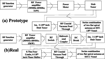
Figure 2. Schematic block diagram of (a) prototype RF system for SST-1/8 and (b) real RF system for SST-1 vacuum vessels.
Download figure:
Standard image High-resolution imageFigure 2(a) shows the schematic block diagram for the prototype RF system. It shows that the RF function generator drives an RF power amplifier within a frequency range of 30 MHz–65 MHz and the maximum RF power output is 1 kW. A power meter is used to measure the forward and reflected power. A coaxial RF vacuum feed-through is used to launch RF power to the antenna inside the SST-1/8 vacuum vessel. Here, a 3-1/8-in., 1 m stub tuner combined with a flexible RFcoaxial cable (1 kW rating) is used for an impedance matching that of the power line. A flexible RFcoaxial cable with a 1 kW rating is used in the rest of the power line.
Similarly, figure 2(b) shows a schematic block diagram of the real RF system. The same RF function generator is used to drive the RF power amplifier within the frequency range of 30 MHz–65 MHz with a maximum RF power output of 15 kW. In the real system, the power line is made of a 3-1/8-in. rigid coaxial line with a two-input and one-output 3-1/8-in. rigid coaxial RF switch, a bi-directional coupler to measure forward and reflected power, a matching network combination of a 6-1/8 in. four limb (each 0.75 m length) phase shifter and a 3-1/8-in. stub tuner of 2 m length, and a 6-1/8-in. coaxial RF vacuum feed-through for launching RF power to the antenna inside the SST-1 vacuum vessel.
Both the prototype and the original antennas are made of two series of Archimedean flat spiral antennas with center-to-center separation of 70 mm. The diameter of each spiral antenna is 200.5 mm, and the gap in between two consecutive arms is 9.5 mm. The arm width and breadth are 8 mm and 10 mm respectively. Each spiral antenna is made of SS-304 and has a 1.98 m electrical length. Figure 3(a) shows the antenna characterization of both the prototype and real antennas in air in terms of the measured profile of the frequency versus reflection coefficient  dB by a VNA (vector network analyzer). In both cases, the profiles are closely matching at several discrete peaks in the range of 25–800 MHz. Figures 3(b) and (c) show similar conditions for the prototype and real RF systems at 52.145 MHz and 50.571 MHz respectively. The derivation shows that the antenna efficiency for the real RF system in a vacuum is
  , where the dissipated resistance for the whole RF power line
  and taking the vacuum radiation resistance as
  , assuming 10% reflection in line. Figure 3(d) shows the plasma discharge produced by the prototype antenna system inside the SST-1/8 vessel at the hydrogen filling pressure of
  mbar. Plasma is produced by the real antenna system inside the SST-1 vessel at hydrogen filling pressure
  mbar, shown in figure 3(e).

Figure 3. Frequency versus reflection coefficient for antenna characterization of (a) prototype (black line) and real (red line) antenna systems, matched state for (b) prototype antenna within SST-1/8 vacuum vessel, (c) real antenna within SST-1 vacuum vessel and plasma discharge by (d) prototype RF system for  mbar filling pressure, (e) real RF system for
  mbar filling pressure of hydrogen at SST-1/8 and SST-1 vacuum vessels respectively.
Download figure:
Standard image High-resolution imageExperiments have also been carried out to excite the higher-frequency peaks to the prototype antenna. Figure 4(a) shows the antenna characteristics in the matched condition at 203 MHz. Figure 4(b) shows that the plasma discharge is produced by launching 203 MHz at a hydrogen filling pressure of  mbar. Figure 4(c) shows the antenna characteristics in the matched condition at 407 MHz. Figure 4(d) shows that plasma discharge is produced by launching 407 MHz at a hydrogen filling pressure of
  mbar.
mbar.

Figure 4. (a) Matched condition, (b) plasma discharge at 203 MHz and (c) matched condition, (d) plasma discharge at 407 MHz by the prototype RF system for the SST-1/8 vacuum vessel at  mbar filling pressure of hydrogen.
Download figure:
Standard image High-resolution image4. Results and discussions
Low loop voltage RF-assisted plasma current start-up in the SST-1 is the ultimate goal; however, in this article, only RF-produced plasma as a preionization mechanism is presented. The necessary and sufficient conditions for plasma breakdown are revisited to understand the overall mechanism. The necessary condition is ionization time  loss time
  and the sufficient condition is plasma breakdown time
  loss time
 for plasma breakdown.
  not only depends up on the necessary condition, but also on the initial electron density at t = 0 or the pre-ionized density
  . At the breakdown time, the electron density
  reaches the critical electron density
  , where the electron–atom collision frequency
  is equal to the electron–ion collision frequency
  [7, 8]. The electron density at time t is
  , where
The plasma breakdown can be thermal or runaway dominated. The thermal regime is a collisional-dominated regime, but the runaway regime is non-collisional. The SST-1 has a major radius of  m, a minor radius of a = 0.2m, and a loop voltage inside the vessel of
  V, which corresponds to an electric field of E = 0.58 V m−1. It is a known fact that the runaway regime would dominate the breakdown if the electric field satisfied the criterion
  (V m−1) [9], where p is the filling pressure in Torr (1 Torr = 133.32 Pa). Therefore, for an available operating E = 0.58 V m−1, the runaway breakdown would be dominated at a pressure of
  Torr. In tokamaks, it is advisable to avoid these E and p conditions as suppression of runaway electrons would be very difficult in a later stage of the discharges. Therefore, tokamaks must be operated in the thermal breakdown regime.
Thermal breakdown obeys the Townsend avalanche criterion. The condition for the allowable error field for reliable Ohmic breakdown is  (V m−1) [9–11]. For reliable Ohmic breakdown in SST-1, the error field should be
  G. Also, the minimum start-up electric field for the thermal-dominated breakdown can be computed by
  (V m−1) =
  , where L is the connection length and
  . Here,
  is effective distance and
  is the error field. At the machine center, the connection length is L = 60 m for
  T and
T and  G for the circular plasma, where
  m [8, 9].
Figure 5 shows a plot of pressure versus minimum electric field  (V m−1) =
  (V m−1) for the thermal breakdown at L = 60 m as well as for the runaway breakdown for the minimum electric field of
  (V m−1). It is revealed that the minima of the minimum electric field requires
  (V m−1) at
  Torr considering thermal breakdown. With the available electric field of E = 0.58 V m−1 within the SST-1 vacuum vessel, some RF-assisted breakdown and current start-up must be required. Also, this shows that runaway breakdown will occur for a filling pressure of
  Torr for
  V m−1.

Figure 5. Plot of pressure versus minimum electric field for thermal and runaway discharges.
Download figure:
Standard image High-resolution imageAlso, successful breakdown requires minimizing the error field through tweaking external coil currents, as well as providing a sufficient pre-ionization electron density  . Let us estimate
  through the preionization mechanism via the RF source considering the error field
  G. The ionization time for RF discharge is usually
  S. On the other hand,
  is mainly dominated by the error field. It is shown that
  S for
S for  G,
G,  T with a filling pressure of
  Torr [8, 9]. The critical density for thermal breakdown is
  , where the neutral density
  . It is seen empirically that the value of
  can be taken for the hydrogen gas discharge at room temperature,
  K. Therefore, the required critical electron density for a filling hydrogen gas pressure of
  Torr is
  . The sufficient condition for the breakdown time is derived from the expression
The calculation shows  S for
S for  , and
, and  S for
S for  , where
  S and
S and  . Therefore, the sufficient condition is satisfied for both values of the preionized electron density for the error field of 50 G. If the error field is lower than 50 G, then breakdown will occurwith even lower values of preionized electron density.
As mentioned, hydrogen plasma discharge has been achieved without a background magnetic field in the SST-1/8 vacuum vessel section. Two flat spiral antennas in a series combination were used to launch the RF power of 800 W at 60 MHz inside the vacuum vessel. The usual background pressure and hydrogen filling pressure of the vacuum vessel were maintained at 10−5 mbar and  mbar (1 mbar = 100 Pa) respectively. The plasma density was measured using a single Langmuir probe of 3 mm and a diameter of around 1 mm. The probe was kept at a distance of 50 mm from the antenna system. The Langmuir probe was operated in an ion saturation regime and biased at −160 V with respect to the vessel. Figure 6 shows the temporal evolution of the ion saturation current of the Langmuir probe of a typical RF discharge plasma. The calculated [12] plasma density of 8.39 × 10¹⁵ m
 m−3 has been achieved from the ion saturation current considering electron temperature of T
 = 3 eV ,which is normal for RF discharge plasma.

Figure 6. Temporal profile of the ion saturation current of the Langmuir probe for an RF discharge in the SST-1/8 vessel.
Download figure:
Standard image High-resolution imageSince the Langmuir probe was unavailable in the vicinity of the antenna system where the RF plasma discharge was produced inside the SST-1 vacuum vessel by launching an RF power of 500 W at the frequency of f = 35 MHz without any background magnetic field, the plasma density was estimated by a spectrograph, which was directly focused on the central plasmas created in between the two spiral antennas. Figure 7 shows that the spectroscopy was set up with AvaSpec-3648 spectrometer where its resolution is 2.37 nm at a slit width of 100 µm, which was measured by a standard Hglamp. In these experiments, the background pressure and hydrogen filling pressure were maintained at 10−6 mbar and 10−3 mbar respectively. Therefore, the background air gas particle and hydrogen gas particle density at room temperature of 300°K were estimated from the ideal gas law  as
as  and
and  respectively. The plasma density and electron temperature are estimated through spectroscopy data. The line spectrum was recorded by the AvaSpec-3648 spectrometer with a set instrumental resolution of 2.37 nm. Mainly, H
 and H
and H line radiations were chosen to calculate the plasma density and electron temperature. Figure 8 shows a typical example of line radiation for the RF plasma discharge obtained in the experiments.

Figure 7. (a) Spectroscopy set up, (b) instrumental width.
Download figure:
Standard image High-resolution image
Figure 8. (a) Line radiation intensity profile, (b) H line radiation intensity profile, (c) H
 line radiation intensity profile for an RF discharge in the SST-1 vessel.
Download figure:
Standard image High-resolution imageIn order to derive the parameters from line radiation, an appropriate spectroscopic model based on either the Corona model or the local thermodynamic equilibrium (LTE) should be checked. The line radiation comes from the transitions of the atoms from theirexcited states to lower states. The spontaneous transitions dominate for the transitions of excited atoms from higher excited states to lower states in the Corona model, whereas the transitions in the LTE model are considered to be mainly due to the collisions. The LTE model is mainly applicable in high-density laboratory plasmas where collisions are high, and sometimes called collision-dominated or CD. The principle of Griem [13] on the validity of LTE model is that the electron collision rates for the transition of the largest energy gap of the considered atoms should be at least 10 times higher than the corresponding spontaneous radiation rate, which is

where  correspond to the ion density of charge state z, electron density, rate coefficient for the collision transition from the higher state p to lower state q and the spontaneous transition probability from the higher state p to lower state q. The LTE model requirement can be derived from this condition considering the average Gaunt factor = 0.2, and it is
The conditions show that  for
for  eV in the application of the LTE model for the considered hydrogen plasma, where the largest energy gap is E(2)–E(1) = 10.2 eV, which lies in between the first excited state energy (E(2)) and ground state energy (E(1)) of hydrogen atoms. Therefore, the LTE model is not suitable for a neutral hydrogen gas particle density of the order of
  . Another possibility is to examine the applicability of the partial local thermodynamic equilibrium (PLTE) model—a more practical concept than the LTE model. The system starts to deviate from the local thermodynamic equilibrium with decreasing electron density that begins from its largest energy gap, which is the energy gap in between the first excited state and the ground state for hydrogen- or helium-like atoms. Still, the LTE model can be applied to higher states where the collisional depopulation can be 10 times higher than the spontaneous decay. Griem defined a level [14] or a principal quantum number as a thermal limit(
 ) such that the collisional depopulation rate is 10 times higher than the spontaneous decay rate for any principle quantum number n where
  . Fujimoto and McWhirter [15] gave a more accurate expression of
  for given
  ,
,  and the charge state z + 1 where z start from zero and
The calculation shows  for the present case of neutral hydrogen (z = 0) with
  and
and  eV. Since the Hα
and Hβ
lines are considered for the calculation, the Corona model would be more appropriate than the PLTE model.
eV. Since the Hα
and Hβ
lines are considered for the calculation, the Corona model would be more appropriate than the PLTE model.
The spontaneous transition is mainly dominated in the Corona model, which can be written in terms of the equilibrium state:
where  represents the summation of all possible transition probabilities from higher state p to all lower states. Therefore, the radiation intensity for the transition from the higher excited energy level p to lower energy level q is
For near-threshold excitation [14], it can be written as
where  . Here, fnm
, EH
, a0,
. Here, fnm
, EH
, a0,  , Emn
correspond to the absorption oscillator strength for n to m transition, ionization energy of hydrogen, Bohr radius, effective Gaunt factor and energy difference between the higher energy state (m) and lower energy state (n) successively. The expression Ipq
can be rewritten as
, Emn
correspond to the absorption oscillator strength for n to m transition, ionization energy of hydrogen, Bohr radius, effective Gaunt factor and energy difference between the higher energy state (m) and lower energy state (n) successively. The expression Ipq
can be rewritten as
where  and
and
If Npq represents the number of photons per unit volume per second due to p to q transitions, then

Therefore, the total number of photons per unit time is collected by the spectrometer is the volume integration of

along the line of sight of the spectrometer. Now, considering that ne
,  are almost constant throughout the plasma volume then
  can be written as

The AvaSpec-3648 measured the intensity in units of (number of photons)/ , and therefore it is required to take the area under the curve of a specified profile of the line radiation of interest and multiply it with the projected area of the plasma volume to obtain the total number of photons per unit time.
Now, the plasma electron temperature ( ) and density(n) are derived from the above formulations using the absolute values of the intensity of the experimental measurements taken by the spectrometer. The intensity ratio of Hα
to Hβ
is used to derive the electron temperature, and the absolute value of intensity of Hα
or Hβ
is used to derive density. At first, the electron temperature will be derived and using that value in the absolute intensity of either Hα
or Hβ
, the plasma density will be calculated.
) and density(n) are derived from the above formulations using the absolute values of the intensity of the experimental measurements taken by the spectrometer. The intensity ratio of Hα
to Hβ
is used to derive the electron temperature, and the absolute value of intensity of Hα
or Hβ
is used to derive density. At first, the electron temperature will be derived and using that value in the absolute intensity of either Hα
or Hβ
, the plasma density will be calculated.
The ratio of Hα
intensity  to Hβ
intensity
to Hβ
intensity  is expressed as
The values of γ, f and E are calculated by taking data from the NIST database [16] where the numbers 1, 2, 3, 4 present the energy levels of the hydrogen atom: n = 1, n = 2, n = 3 and n = 4 respectively. For a typical example, figure 8 shows  . It is observed that the spread of electron temperatures for different discharges is approximately 2 eV–6 eV. Plasma density is calculated for the typical example of figure 8 by taking the electron temperature of
  eV. In this derivation of the plasma density, singly ionized plasma is considered, with an electron temperature of around 3 eV and the second ionization potential for hydrogen-like atoms such as nitrogen, carbon and oxygen is high. Therefore, the quasineutrality condition
  for z = 1 is applied and the plasma density upper and lower limits are derived from both the absolute value of
  and
and  . The values of the upper and lower limits of the plasma density from both derivations are compared.
The theoretical expressions of  and
and  are represented as
and
Here, n0 is the neutral particle density in the plasma state, and the line-of-sight volume of the spectrometer is  . For the typical example of figure 8, the experimental measured values are
  and
and  , which are obtained by taking the area under the measured profile of Hα
, Hβ
and multiplying them by the multiplication factor 20
, which are obtained by taking the area under the measured profile of Hα
, Hβ
and multiplying them by the multiplication factor 20  .
.  is obtained after putting all the values in
  . Similarly,
  is obtained by putting all the values in
  . Both of these derivations show that
  are very close to each other and hence the average value used is
  . Since n0 is the neutral particle density in the plasma, from the particle conservation law
  , where nn
is the neutral particle density at the filling pressure of hydrogen gas. So, the solution of the quadratic equation is
, where nn
is the neutral particle density at the filling pressure of hydrogen gas. So, the solution of the quadratic equation is ![$n_\mathrm{e} = \frac{n_\mathrm{n}}{2}\left[1\pm\sqrt{1-\frac{4s}{n_\mathrm{n}^{2}}}\right]$](https://content.cld.iop.org/journals/0741-3335/64/1/015004/revision2/ppcfac3498ieqn121.gif) , where
, where  and
and  . Considering the + sign, the upper density limit is
  and with the − sign, the lower density limit is
  . So, the plasma density remains in between the two limits
  and
and  .
.
Broadening features of the Hα
and Hβ
lines are also examined based on line-broadening data as shown in figure 9. Both Hα
and Hβ
line profiles are very well fitted with both with a Gaussian function of  and Lorentzian function of
  , where FWHM for the Gaussian profile is
  and for the Lorentzian profile is wL
. The Gaussian and Lorentzian widths of the Hα
profile are 2.8 nm and 2.7 nm respectively and the same for the Hβ
profile are 2.67 nm and 3.23 nm respectively. Both the line profiles of Hα
and Hβ
are broadened since the instrumental width is 2.37 nm. Doppler broadening gives the temperature of the atoms and the Doppler broadening from Gaussian width (FWHM) is represented as
and for the Lorentzian profile is wL
. The Gaussian and Lorentzian widths of the Hα
profile are 2.8 nm and 2.7 nm respectively and the same for the Hβ
profile are 2.67 nm and 3.23 nm respectively. Both the line profiles of Hα
and Hβ
are broadened since the instrumental width is 2.37 nm. Doppler broadening gives the temperature of the atoms and the Doppler broadening from Gaussian width (FWHM) is represented as  [17]. The temperature of hydrogen atoms for 1 nm Doppler broadening is
  , which is quite a large temperature and not realistic for the present scenario. Therefore, the experimental profile is not comprised only of a Gaussian profile. So, the profile is a convolution of Gaussian and Lorentzian profiles. The Lorentzian broadening and Gaussian broadening are obtained through the deconvolution procedure based on the Voigt fitting profile [18]:

The Gaussian width can be written in terms of instrumental width (wI
) and Doppler broadening ( ) as
) as  . Here,
  and
and  are varied to obtain the best Voight fit with the experimental profiles of Hα
and Hβ
. It has been seen that the best Voight fitting is achieved at
are varied to obtain the best Voight fit with the experimental profiles of Hα
and Hβ
. It has been seen that the best Voight fitting is achieved at  and
and  for the Hα
profile and
for the Hα
profile and  and
and  for the Hβ
profile for the example of figure 9. The temperature of neutral atoms has been found from Doppler broadening after de-convolution of the instrumental width from the Gaussian width of Hα
and Hβ
lines respectively, which are
for the Hβ
profile for the example of figure 9. The temperature of neutral atoms has been found from Doppler broadening after de-convolution of the instrumental width from the Gaussian width of Hα
and Hβ
lines respectively, which are  from Hα
and
from Hα
and  from Hβ
. The temperature of neutral atoms calculated from Hα
is quite high. Sincethe experiment has been carried out using a relatively poor resolution spectrometer (2.37 nm), it is important to check the contributions from strong line radiations originating from C, N and O as well as their first ionized states. It has been confirmed from NIST data set that the radiation line 657.8 nm from C+ can contribute within the Hα
intensity profile. This may be the reason for the higher Gaussian width and consequently higher neutral particletemperature. On the other hand, all of the strong spectral lines originating from C, N and O and from their first ionized states are located far from the Hβ
line such that those lines can not affect the Hβ
line width according to the NIST data set. The calculated temperature of the same from Hβ
may possibly be due to anomalous heating.
from Hβ
. The temperature of neutral atoms calculated from Hα
is quite high. Sincethe experiment has been carried out using a relatively poor resolution spectrometer (2.37 nm), it is important to check the contributions from strong line radiations originating from C, N and O as well as their first ionized states. It has been confirmed from NIST data set that the radiation line 657.8 nm from C+ can contribute within the Hα
intensity profile. This may be the reason for the higher Gaussian width and consequently higher neutral particletemperature. On the other hand, all of the strong spectral lines originating from C, N and O and from their first ionized states are located far from the Hβ
line such that those lines can not affect the Hβ
line width according to the NIST data set. The calculated temperature of the same from Hβ
may possibly be due to anomalous heating.

Figure 9. (a) Gaussian, (b) Lorentz, (c) Voight fit of H line radiation profile and (d) Gaussian, (e) Lorentz, (f) Voight fit of H
 line radiation profile for a typical RF discharge plasma in the SST-1 vessel.
Download figure:
Standard image High-resolution image
When the Lorentzian width is considered for both Hα and Hβ , it is observed that the Lorentzian width of Hβ is always greater than the Hα line. Lorentzian broadening can occur due to pressure broadening by neutral particles or through the Stark effect due to electric fields. Pressure broadening due to ground state atoms can be written as follows [17]:
Calculations show that  is required for
  nm or 1 nm pressure broadening. So, pressure broadening is not applicable for the present scenario.
Stark broadening can also be considered to confirm Lorentzian broadening. Stark broadening occurs due to either electron impact of the passing of high-speed electrons near the excited atoms, microfields generated by static ions, slow ion movement, a highly intensified oscillating electric field due to antenna radiation, the turbulent electric field present in the system, or the sum of all these effects. The Lorentzian width of the Hβ
line is higher than that of the Hα
line, which is consistent with Stark broadening. Stark broadening due to electron impact can be represented as [17]  . The electron density is estimated
  for
for  nm, which turns out to be high in the present scenario, and therefore electron impact broadening is not responsible alone for Stark broadening.
The calculation of the microfield due to static or slow moving ions near the radiator can be calculated from the quasi-static approximation of the standard theory model of Griem [19]. In order to obtain the microfield, the Holtsmark field [14, 17, 20] is calculated, which is expressed as  . For hydrogen plasma z = 1, and if the plasma density is taken as
  , then the finite Holtsmark field would be
  V m−1. The Holtsmark field F0 is related to the average microfield
  [21], which is
  V m−1 and can contribute to finite Stark broadening. Considering Debye shielding with the electron temperature effect, Hooper [22] calculated a microfield distribution in plasma for different a with the parameter
  . Now,
  is the ion–ion minimum distance, which can be calculated from
  , and
, and  is the Debye radius, which is
  . In the present case, calculations show that a = 0.06 for
  and
and  . The Holtsmark field distribution profile is related to
and normalized field  with
with  . Here, graphically
  determines strong Stark broadening, which is the asymptotic expansion of this distribution; for the large
  , the Holtsmark field expression simplifies to
  . The asymptotic expansion starts for any parametric values of a when β = 6. Considering strong Stark broadening at β = 6, the
  V m−1 is close to the average microfield
  V m−1 calculated from the Holtsmark field distribution. Satisfactory Stark broadening could be obtained when the ion microfields are larger than the ion field within the Debye sphere and the condition [19] is
  , where
  is the total number of ions within the Debye sphere. Calculations show that
  . Therefore, the ion density
  with
with  eV may produce finite Stark broadening, but the amplitude of the microfield is not sufficient to produce the observed Stark broadening of the width 0.51 for the present scenario.
The RF electric field oscillations in the vicinity of the antenna are calculated from the time-averaged Poynting vector

and it can be superimposed on the static microfield. The average power radiated by the antenna [23] is given by
which can be simplified as  , where S is the surface area of the antenna and η is the intrinsic impedance of the medium. Now, the antenna has a radius of 10.9 cm and
  ,
,  V m−1 for the input power of 500 W at fully matched conditions. If the power is concentrated more towards the antenna center, then E0 will be higher.
The RF oscillating electric field and microfield are not sufficient for the present scenario for Stark broadening. Both the microfield and electron impact effects may have a combined effect as explained by Standard Theory [19, 24], but this is not applicable here due to the low plasma density and temperature. Thus, the only remaining possibility is the presence of a turbulent electric field in the system to explain this scenario.
The Stark effect is also reported by Blochinzew [25]; therein broadening happens due to a low-frequency ion acoustic wave caused by an oscillating monochromatic RF field. In thermal plasmas, the micro field dominates over oscillating RF field, but in turbulent plasmas the oscillating RF field can generate several orders of magnitude due to the nonlinear effect, and a prominent dynamic Stark effect has been observed in the Balmer lines of hydrogen [26, 27]. So, the possibility of a turbulent field effect causing higher Stark broadening can not be ruled out in the present scenario. The present scenario will now be examined.
In the present case, the experiment is conducted in the absence of a background magnetic field where electrons are not confined. So, electrons can move randomly with their speeds determined by the electron temperature. To maintain quasineutrality within the plasma, an ion acoustic wave can be excited. In addition, the oscillating RF electric field may also couple non-linearly for a stimulating ion acoustic wave. To excite a linear ion acoustic wave, the required perturbing electric field can be calculated from the expression  . If it is considered that perturbing density is
  10% and
  cm−1, then
  = 30 V m−1 for
  = 3 eV. The magnitude of the RF electric field is
  V m−1, which is 100 times greater, and there is a large probability of creating nonlinear coupling in between the RF oscillating electric field and the perturbing electric field of ion acoustic wave, which may create a large nonlinear effect and may reflect Hβ
line broadening. The neutral atom temperature from the Hβ
line is
V m−1, which is 100 times greater, and there is a large probability of creating nonlinear coupling in between the RF oscillating electric field and the perturbing electric field of ion acoustic wave, which may create a large nonlinear effect and may reflect Hβ
line broadening. The neutral atom temperature from the Hβ
line is  eV. The temperature of neutral particles are generated through the ion neutral collisions where ions gain energy from the electric field. If the anomalous neutral particle energy from the wave turbulent RMS electric field
  is calculated, then it can be written as
  . Now,
  V m−1 = 37.6 kV cm−1 for the
  and
and  eV. This value of the turbulent electric field is sufficient to produce a Stark broadening width of
  for the present scenario, which is consistent with similar observations like in the T-10 Tokamak, Alcator C-Mod, etc [28, 29].
5. Conclusions
An alternate method for the RF plasma pre-ionization and current start -up has been presented for the SST-1. This would possibly be an alternative of the present method that assists the pre-ionization and current start-up with a 42 GHz ECRH system with 500 kW, capable of providing the launch of ECR waves in the second harmonics at 0.75 T and a fundamental frequency at 1.5 T. The flat spiral antenna system has been extensively tested in a 1/8th section of a SST-1 vacuum chamber as well as in the SST-1 vacuum vessel. This antenna assembly would be able to operate at the toroidal magnetic field of up to 3 T, so that the present limitations using the ECR system up to 1.5 T would not be a problem. The results obtained through the Langmuir probe are encouraging, measuring the RF plasma density at the 1/8th section of SST-1 vacuum vessel of around  (measured 50 mm away from the antenna system), whereas the spectroscopic estimation shows that the plasma density will at least be higher than
  and
and  –6 eV at the SST-1 vessel for the applied RF energy of around 500 W. Both these results show that the antenna system should be capable enough of creating a successful low loop voltage breakdown and current start-up in SST-1. In addition, the effect of the magnetic field producing RF discharge plasma is very important due to the confinement of the stray electrons; also, most of the charged particles remain confined by the background magnetic field at the time of the breakdown. Without a background magnetic field, there is a large probability that electrons can lose isotopically by absorbing energy from the RF electric field without any collisions with neutrals, and therefore plasma breakdown is relatively tough without a background magnetic field compared to with a background magnetic field. It is also observed that the anomalous neutral particle temperature due to the presence of the turbulent electric field is of the order of 106 V m−1 at the antenna center in the SST-1. A possible mechanism of this strong turbulent wave electric field is ion acoustic wave excitation from the initial perturbation of the RF oscillating field as well as the random movement of electrons due to a lack of background magnetic field. The plasma discharge is also achieved at a hydrogen gas fill pressure of
  mbar with RF power 1.5 kW without a background magnetic field. There is scope for further increasing the RF power during the breakdown phase of the SST-1 in order to produce reliable thermal plasma breakdown at the fill pressure range of
  mbar with a background toroidal magnetic field of
  –3 T.
–3 T.
Acknowledgments
We would like to acknowledge DAE for supporting this work. The first author also would like to acknowledge the IPR Mechanical Engineering Service Division for the support and help during the spiral antenna fabrication and commissioning phases. Particularly, special thanks to Vinod D Kaila from the mechanical workshop for his kind valuable help wherever and whenever required during the antenna fabrication and assembly. We would also like to thank Nilam K Ramaiya, Nandini Yadava, Malay Bikas Chowdhuri and Ranjana Manchanda for help in obtaining the spectroscopy data.
Data availability statement
The data generated and/or analysed during the current study are not publicly available for legal/ethical reasons but are available from the corresponding author on reasonable request.