Parallelizing Particle Swarm Optimization in a Functional Programming Environment

Abstract

Many bioinspired methods are based on using several simple entities which search for a reasonable solution (somehow) independently. This is the case of Particle Swarm Optimization (PSO), where many simple particles search for the optimum solution by using both their local information and the information of the best solution found so far by any of the other particles. Particles are partially independent, and we can take advantage of this fact to parallelize PSO programs. Unfortunately, providing good parallel implementations for each specific PSO program can be tricky and time-consuming for the programmer. In this paper we introduce several parallel functional skeletons which, given a sequential PSO implementation, automatically provide the corresponding parallel implementations of it. We use these skeletons and report some experimental results. We observe that, despite the low effort required by programmers to use these skeletons, empirical results show that skeletons reach reasonable speedups.

1. Introduction

Evolutionary and swarm metaheuristics [1,2,3,4,5,6,7] provide generic solutions to face hard computational problems. They are based on making some simple entities interact with each other according to some simple rules, in such a way that the solution or set of solutions iteratively improves. Since interactions between entities are simple and local, typically these algorithms can be efficiently parallelized, reaching reasonable speedups: if (sets of) entities are assigned to different processors, then the overhead due to the communications between (sets of) entities at different processors might be a small proportion of all necessary computations. Several parallel schemes for implementing these methods have been proposed [8,9,10,11,12,13].

In both sequential and parallel bioinspired algorithms, finding the suitable metaheuristic for each problem is not an easy task. Many methods work fine for some problems but provide poor results for other problems. Thus, if a given problem is intended to be solved by using these methods and some minimum optimality level is required, then the programmer must invest some time implementing different algorithms (or adapting available metaheuristic frameworks to the problem under consideration) and checking which one performs best for the problem under consideration. Due to the additional difficulties of parallel programming, this investment is even higher if a parallel approach is intended to be used.

Functional programming [14] is a programming paradigm where, after the initial learning curve, complex programs can be written in short time compared to other paradigms. The higher-order nature of functional languages, where programs (functions) can be treated as any other kind of program data, make them very useful to implement generic programming solutions which can be trivially reused for other problems. This is even clearer in parallel programming. Since programs can trivially refer to themselves, the coordination of parallel subcomputations can be defined by using the same constructions as in the rest of the program. This enables the construction of skeletons [15], which are generic implementations of parallel schemes that can be invoked in run-time to immediately obtain a parallelization of a given sequential program. The skeleton defines how subcomputations coordinate in parallel, and the skeleton user just has to define (part of) the subcomputations.

Several parallel functional languages have been proposed (see, e.g., [16,17,18,19,20,21]). In this paper we show how to use one of them to simplify the development of parallel versions of a swarm optimization method. In particular, we use the language Eden [17,22], a parallel version of Haskell [23], to create a generic skeleton implementing the parallelization of Particle Swarm Optimization (PSO) [24,25,26,27,28,29,30], which is one of the most essential methods in swarm optimization. However, the main ideas presented in the paper can also be applied to deal with other bioinspired methods. In fact, this work continues our project to develop Eden skeletons for several kinds of bioinspired methods, which began in [31] by the introduction of an skeleton to parallelize genetic algorithms [32].

We present some Eden skeletons to parallelize Particle Swarm Optimization. Note that skeletons allow us to quickly compare not only different parallel metaheuristics, but also different strategies to parallelize the same metaheuristic. For instance, in one of these skeletons, the operation of updating the best solution found so far at all processes is not performed every execution iteration, but it is constrained to some specific times. Thus, particles assigned to each processor (particle islands) evolve more independently, which reduces the communication overhead and improves the speedup. The performance of these skeletons is tested for several PSO instances, and we report experimental results. Empirical results show that users of our skeletons can obtain reasonable speedups with very small programming effort. Thus, any programmer without large expertise on parallel programming can easily benefit from our parallel skeleton, whose clear modularity enables a fast and easy adaptability to any kind of problem under consideration.

In the literature we can find different types of parallel languages using very different levels of control over parallelism. Languages range from completely explicit parallelism, where the programmer controls all the details of the parallelization, to completely implicit parallelism, where the compiler automatically exploits the inherent parallelism of the sequential version of the program. Explicit languages allow to obtain better time performance at the cost of more programming effort, while implicit languages reduce the programming effort, though the obtained performance is usually worse. The Eden language tries to find a trade off between both extremes: it is a explicit language where the programmer specifies what is to be executed in parallel, but the compiler deals automatically with many details of the parallelization, like communication and synchronization between processes. Moreover, by using skeletons, we can get the best of both worlds. First, an expert parallel programmer can develop efficient skeletons by making use of explicit parallelism to control all the required details. Second, non expert parallel programmers can directly use the available skeletons, reaching speedups similar to those obtained by explicit languages, though with a programming effort close to that needed by implicit languages, because it is only necessary to replace a sequential function call by the corresponding call to the parallel skeleton.

The main contribution of this paper consists in providing parallel functional skeletons for implementing PSO. The library is publicly available at the web page of the first author of the paper. This contribution is useful for the following reasons:

(a)

The functional paradigm allows programmers to write clean and highly reusable programs with a relatively low effort.

(b)

The skeletons can be used to quickly test the performance of different versions of parallel PSO for the a given problem, thus helping the programmer to decide whether PSO (or a given parallel PSO approach) is the right choice for her problem. Together with other parallel functional skeletons for other metaheuristics (e.g., a skeleton for genetic algorithms was introduced in [31]), programmers will be able to quickly test different parallel metaheuristics for a given problem, compare them, and pick the most appropriate one.

(c)

Using the skeletons does not require programming in Eden, since Eden can invoke functions written in other languages. For instance, after a programmer provides a fitness function written in C, all of these skeletons are ready to be executed.

The rest of the paper is structured as follows. In Section 2 we introduce the main features of the functional languages we will use in the paper. In Section 3 we introduce the Particle Swarm Optimization method. Then, in Section 4, we present how to develop a higher-order sequential Haskell function dealing with particle swarm optimization algorithms. Afterwards, in Section 5 we introduce several parallel versions of such higher-order function. Experimental results are presented and discussed in Section 6. Finally, Section 7 contains our conclusions and lines of future work.

2. Functional Languages under Consideration

In this section we introduce the functional languages used in the paper. First, we introduce the sequential functional language Haskell, and then we present its parallel extension Eden.

2.1. Brief Introduction to Haskell

The core notion of functional programming is the mathematical function, that is, a program is a function. Complex functional programs are created by starting with simple basic functions and using functional composition. Haskell is the de facto standard of the lazy-evaluation functional programming community. It is a strongly typed language including polymorphism, higher-order programming facilities, and lazy order of evaluation of expressions. Lazy evaluation is an evaluation strategy which delays the evaluation of each expression until the exact moment when it is actually required.

As it can be expected, the language provides large libraries of predefined functions, and also predefined data types for the most common cases, including lists. Let us remark that Haskell provides polymorphism. Thus, data types can depend on other types. For instance, the programmer can define a generic type to deal with binary trees of any concrete type a:

          data Tree a = Empty | Node a (Tree a) (Tree a)
        

New functions can be defined by analyzing cases on the structure of the data types. For instance, the following function computes the total number of elements of any tree (of any concrete type) by using pattern matching:

          length :: Tree a -> Int
          length Empty = 0
          length (Node x t1 t2) = 1 + length t1 + length t2
         

The first line of the definition is optional, and it represents the type declaration of the function: Given a tree of any concrete type a, it returns an integer. The rest of the definition represents the definition of the behavior of the function: If it receives an empty tree, then it returns 0; otherwise, it adds 1 to the sum of the lengths of both subtrees.

Structures like binary trees are potentially infinite. Usually, a computation over such infinite structure would imply the evaluation of the whole structure, that is, it would mean the non-termination of the program. How can we manage with them? Haskell provides a very powerful tool to treat this type of structures: laziness. When an expression is not needed, thanks to laziness it is not evaluated. In particular, the evaluation is driven by demand. For instance, let us consider the following definition of an infinite binary tree:

          infTree :: Tree Int
          infTree = Node 1 infTree infTree
        

and the following function to know whether a binary tree is empty or not:

          emptyTree :: Tree a -> Bool
          emptyTree Empty = True
          emptyTree (Node a b c) = False
       

Knowing whether the binary tree

          (Node 1) infTree infTree
        

is empty or not is possible because, thanks to laziness, both subexpressions infTree of

          emptyTree ((Node 1)infTree infTree)
       

remain unevaluated.

Other powerful characteristic of Haskell is higher-order. It means that functions can be arguments of functions. For instance, the following predefined function map receives as input a function f and a list, and then it applies function f to every element of the list:

          map :: (a -> b) -> [a] -> [b]
          map f [] = []
          map f (x:xs) = (f x):(map f xs)
       

Notice that the type declaration of function map indicates that its first parameter has type a->b, denoting that the first parameter is a function that receives values of type a and returns values of type b. The second parameter is a list of elements of type a, and the result is again a list, but in this case of elements of type b.

It is also possible to define functions dealing with lists by using comprehension lists. For instance, the previous map definition is equivalent to the following one:

          map :: (a -> b) -> [a] -> [b]
          map f xs = [f x | x <- xs]
         

Notice that, in higher-order languages like Haskell, it is also possible to deal with partially applied functions. For instance, map can take as its functional argument a partial application of function (+):

          mapPlusOne :: [Int] -> [Int]
          mapPlusOne xs = map (1+) xs
        

Thus, it adds one to each element of the list.

Let us remark that functions like map can be used to deal with lists of any type. However, sometimes it is also useful to have functions that can deal with many types but not all of them. For instance, if we want to sort a given list, we can only do it in case the elements of the list belong to a type where we can compare elements. Haskell deals with this issue by defining classes of types. For instance, function sort only works for lists whose basic type belongs to class Ord:

          sort :: Ord a => [a] -> [a]
          sort [] = []
          sort (x:xs) = (sort [y|y<-xs,y<x]) ++ [x] ++ (sort[y|y<-xs,y>=x])
        

New type classes can be defined by programmers. They only need to specify what basic operations are required to belong to the class.

2.2. Introduction to Eden

Eden [22,33] is a parallel extension of Haskell. It introduces parallelism by addingsyntactic constructs to define and instantiate processes explicitly. It is possible to define a new process abstraction p by applying the predefined function process to any function \x -> e, where variable x will be the input of the process, while the behavior of the process will be given by expression e. Process abstractions are similar to functions—the main difference is that the former, when instantiated, are executed in parallel. From the semantics point of view, there is no difference between process abstractions and function definitions. The differences between processes and functions appear when they are invoked. Processes are invoked by using the predefined operator #. For instance, in case we want to create a process instantiation of a given process p with a given input data x, we write (p # x). Note that, from a syntactical point of view, this is similar to the application of a function f to an input parameter x, which is written as (f x).

Therefore, when we refer to a process we are not referring to a syntactical element but to a new computational environment, where the computations are carried out in an autonomous way. Thus, when a process instantiation (e1 # e2) is invoked, a new computational environment is created. The new process (the child or instantiated process) is fed by its creator by sending the value for e2 via an input channel, and returns the value for e1 e2 (to its parent) through an output channel.

Let us remark that, in order to increase parallelism, Eden employs pushing instead of pulling of information. That is, values are sent to the receiver before it actually demands them. In addition to that, once a process is running, only fully evaluated data objects are communicated. The only exceptions are streams, which are transmitted element by element. Each stream element is first evaluated to full normal form and then transmitted. Concurrent threads trying to access not yet available input are temporarily suspended. This is the only way in which Eden processes synchronize. Notice that process creation is explicit, but process communication (and synchronization) is completely implicit.

2.3. Eden Skeletons

Process abstractions in Eden are not just annotations, but first class values which can be manipulated by the programmer (passed as parameters, stored in data structures, and so on). This facilitates the definition of skeletons as higher order functions. Next we illustrate, by using a simple example, how skeletons can be written in Eden. More complex skeletons can be found in [22].

The most simple skeleton is map. Given a list of inputs xs and a function f to be applied to each of them, the sequential specification in Haskell is as follows:

          map f xs  =  [f x | x <- xs]
        

that can be read as for each element x belonging to the list xs, apply function f to that element. This can be trivially parallelized in Eden. In order to use a different process for each task, we will use the following approach:

          map_par f xs =  [pf # x | x <- xs] `using` spine
            where pf = process f
       

The process abstraction pf wraps the function application (f x). It determines that the input parameter x as well as the result value will be transmitted through channels. The spine strategy (see [16] for details) is used to eagerly evaluate the spine of the process instantiation list. In this way, all processes are immediately created. Otherwise, they would only be created on demand.

Let us note that the Eden’s compiler has been developed by extending the GHC Haskell compiler. Hence, it reuses GHC’s capabilities to interact with other programming languages. Thus, Eden can be used as a coordination language, while the sequential computation language can be, for instance, C.

3. Introduction to Particle Swarm Optimization

Particle Swarm Optimization [24,25,26,27] (from now on PSO) is a metaheuristic inspired on the social behavior of flocks of birds when flying, as well as on the movement of shoals of fish. A population of entities moves in the search space during the execution of the algorithm. These entities are very simple and perform local interactions. The result of combining simple behaviors is the emergence of complex behaviors and the ability to get good results as a team.

It is assumed that the flock searches for food in an area and that there are some food at each point in the area. It is also assumed that birds in the flock do not know where the maximum amount of food is, but they can see where other birds are, so a good strategy to find a big food source is to follow the bird that found the biggest food source so far. PSO emulates this behavior to solve optimization problems. Each solution or particle is a bird in the search space that is always moving and never dies. In some versions of PSO, birds can actually die. In fact, we can consider that the swarm is a multi-agent system where particles are simple agents that move through the search space and store (and possibly communicate) the best solution found so far.

Each element of the swarm has a fitness value, a position and a velocity vector that directs its flight. The movement of particles is partially guided by the best solution found by all particles. Concretely, a particle $s{w}_i$ is composed of four vectors: (a) Vector $x_i$, which stores the current position (location) of the particle in the search space; (b) vector $v_i$, which stores the velocity vector according to which the particle moves; (c) vector $p_i$, which stores the location of the best solution found by the particle so far; and (d) vector g, which stores the location of the best solution found by the swarm and is common to all entities. It also has three fitness values: (i) $x_i^{fitness}$, which stores the fitness of the current solution ($x_i$ vector); (ii) $p_i^{fitness}$, which stores the fitness of the best local solution ($p_i$ vector); and (iii) $g^{fitness}$, which stores the fitness of the best global solution (g vector).

The movement of each particle $s{w}_i$ depends on the best solution it has found since the algorithm started, $p_i$, and the best solution found by all particles in the entire cloud of particles, g. This kind of particle neighborhood, where all particles in the swarm are attracted to the best solution, is called gbest neighborhood [34]. There exist other kinds of social structures, such as the lbest neighborhood, where each element is guided by the best solution found by its k nearest neighbors. The behavior of other neighborhood topologies has been studied [35]. In particular, it is shown that using an adequate topology is important to obtain good performance, although the best choice depends on the problem being solved. Generally, the gbest topology provides a quick algorithm convergence. According to this topology, the velocity $v_i$ of $s{w}_i$ is changed at each iteration of the algorithm to bring it closer to positions $p_i$ and g.

Given a swarm $sw$ where S is the number of particles in $sw$, the goal is to minimize or maximize a function $f:{\mathbb{R}}^n\to \mathbb{R}$ (hereafter we will assume that the goal is minimizing it). A basic PSO algorithm follows:

 (Initialization)
   For i = 1,…,S  Do
      initPosition(i)
      initBestLocal(i)
      If i = 1  Then initBestGlobal()
      If improvedGlobal(i) Then updateBestGlobal(i)
      initVelocity(i)
    End For
 (While loop)
   While not endingCondition()
      For i = 1,…,S Do
         createRnd(rp,rg)
         updateVelocity(i,rp,rg)
         updatePosition(i)
         If improvedLocal(i) Then updateBestLocal(i)
         If improvedGlobal(i) Then updateBestGlobal(i)
       End For
     End While
      

We comment on the algorithm steps. First, there is an initialization where all $s{w}_i\in sw$ (first For loop) are initialized as it is described next. In initPosition(i), the position $x_i$ of particle $s{w}_i$ is randomly chosen within the range $[bot,up]$, where $bot$ and $up$ are the lower and upper bounds of the search space (note that $bot$ and $up$ can be different for each dimension); this is usually called the dynamic range, and particles cannot move out of these limits. Additionally, we compute $x_i^{fitness}=f\left(x_i\right)$. In the initBestLocal(i) phase, we set $p_i=x_i$ and $p_i^{fitness}=x_i^{fitness}$. The next instruction, initBestGlobal(), is only executed when $i=1$ and initializes $g=x_1$ and $g^{fitness}=x_1^{fitness}$. If improvedGlobal() $=True$, that is, if $p_i^{fitness}<g^{fitness}$, then the best global solution is updated in updateBestGlobal(i), where the following operations are performed: $g=p_i$ and $g^{fitness}=p_i^{fitness}$. Finally, in the initVelocity(i) phase, the particle’s velocity is randomly established in the range $[-|up-bot|,|up-bot\left|\right]$ for each of the dimensions, but usually it is limited by a fixed value, $v_{max}$, which cannot be exceeded.

After the initialization, the core of the PSO method is executed until the endingCondition() is satisfied (While loop). The endingCondition() can limit the number of iterations performed, the time consumed, or the fitness adequation. In the body of the While loop (the For loop), all particles are updated. The first step in the For loop, createRnd(rp,rg), creates two random values ($rp$ and $rg$) in the range (0, 1) that will be used in the next phase. Then, in updateVelocity(i,rp,rg), the velocity of $s{w}_i$ is updated in the following way:

$$v_i=\omega ·v_i+\varphi p·rp·(p_i-x_i)+\varphi g·rg·(g-x_i)$$

where ω is a parameter called inertia weight (introduced in [25]) which influences the convergence of the algorithm: For instance, an excessive inertia value can make the particle systematically exceed the optimum from a side to another in each movement, whereas a low value could make it approach the optimum at a too low pace; $\varphi p$ and $\varphi r$ are called the cognitive and social parameter, and make the method be less predictable and more flexible. $\varphi p$ controls the influence on the movement of the own knowledge of the particle, while $\varphi r$ controls the influence of the global knowledge. All of these parameters are experimentally set (see [29,36,37,38] for further details) and control the behavior and efficacy of the PSO method. The next step, updatePosition(i), updates the position of $s{w}_i$, adding its new velocity to its current position: $x_i=x_i+v_i$, and updates the fitness value by setting $x_i^{fitness}=f\left(x_i\right)$. If $x_{max}$ is exceeded, then we set $x_i=x_{max}$. At the end of the loop, if improvedLocal() $=True$, that is, if $x_i^{fitness}<p_i^{fitness}$, then the best local solution is updated in updateBestLocal(i) as follows: $p_i=x_i$ and $p_i^{fitness}=x_i^{fitness}$. In the last step, if improvedGlobal() is satisfied then the global solution is updated in the updateBestGlobal(i) phase as we explained above.

4. Generic PSO Algorithms in Haskell

Let us note that Haskell functions are first-class citizens. Thus, they can be used as parameters of other functions. In particular, in order to provide a general scheme to deal with PSO algorithms, we need to use as parameter the concrete fitness function used in the problem. In addition to the fitness function, we also need to consider other parameters like the number of particles to be used, the number of iterations to be executed by the program, the boundaries of the search space, and the parameters ω, $\varphi p$ and $\varphi r$ described in Section 3. Moreover, in order to implement PSO in a pure functional language like Haskell, we need an additional parameter to introduce randomness. Note that Haskell functions cannot produce side-effects, so they need an additional input parameter to be able to obtain different results in different executions. Taking into account these considerations, the type of the higher-order Haskell function dealing with PSO algorithms is the following:

        pso :: RandomGen a => a         --Random generator
               -> WPGparams             --ω, ϕ p and ϕ r
               -> Int                   --Number of particles
               -> Int                   --Number of iterations
               -> (Position->Double)    --Fitness function
               -> Boundaries            --Search space bounds
               -> (Double,Position)     --Result:Best fitness and position
      

Note that the type Position should be able to deal with arbitrary dimensions. Thus, the simplest and more general solution to define a position is to use a list of real numbers, where the length of the list is equal to the number of dimensions of the search space. Analogously, the type Boundaries should contain a list of lower and upper bounds for each of the dimensions. Thus, it can be described by a list of pairs of real numbers. Finally, the type WPGparams is even simpler, as it only contains a tuple of three real numbers describing the concrete values of parameters ω, $\varphi p$ and $\varphi r$:

        type Position = [Double]
        type Boundaries = [(Double,Double)]
        type WPGparams = (Double, Double, Double)
      

Once input parameters are defined, it is time to define the body of the function. First, we use function initialize to randomly create the list of initial particles. Its definition is simple, as we only need to create np particles randomly distributed inside the search space defined by the boundaries bo. Once particles are initialized, we use an independent function pso’ to deal with all the iterations of the PSO algorithm. As in the case of the main function pso, the auxiliary function pso’ will also need a way to introduce randomness in order to have appropriate random values for $rp$ and $rg$ in the range (0, 1). This problem is solved by function makeRss, which creates all needed random values.

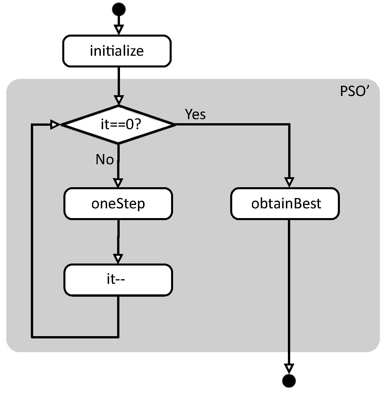
        pso sg wpg np it f bo = obtainBest (pso’ rss wpg it f bo initPs)
          where initPs = initialize sg np bo f
                rss = makeRss np (randomRs (0, 1) sg)
        --Particle: Best local value, best global value, current position and
        --velocity, best local position, best global position
        type Particle = (Double,Double,Position,Velocity,Position,Position)
        type Velocity = [Double]
      

Note that each particle contains its position, its velocity (that will also be randomly initialized), the best solution found by the particle, and the best solution found by any particle.

Function pso’ has a simple definition. It runs recursively on the number of iterations. If there is not any iteration to be performed then we just return as result the input particles. Otherwise, we apply one iteration step (by using an auxiliary function oneStep) and then we recursively call our generic scheme with one iteration less:

        pso’ _ _ 0 _ _ pas = pas
        pso’ (rs:rss) wpg it f bo pas = pso’ rss wpg (it-1) f bo
                                               (oneStep rs wpg f bo pas)
      

Figure 1 summarizes the flowchart of function pso. First, function initialize creates the initial conditions to start the evaluation, and then function pso’ performs the real work. In this case, pso’ is executed while the number of remaining iterations is not zero, calling the auxiliary function oneStep in each iteration. When the iterations are finished, function obtainBest returns the best solution found so far.

Let us now concentrate on how each step is performed. First, each particle is updated. This is done by function updateParticle, that applies the equations described in Section 3 to update the velocity and position. Moreover, this function also checks if the fitness of the new position is better than the best solution found so far. Thus, the output of the function is a list of pairs (Bool, Particle) where the boolean value is True if the new position of the particle is better than the best position found globally so far. Once all particles have been updated, we check if any of them have improved the best solution or not. If some particles have improved the best solution, we sort the new best solutions and select the new best one. Finally, all particles are updated with the information about the new best global position. The next code shows how each step is done:

        oneStep :: [(Double,Double)] -> WPGparams -> (Position -> Double)
                   -> Boundaries -> [Particle] -> [Particle]
        oneStep rs wpg f bo pas
          |null newBests = newPas
          |otherwise = map(updateGlobalBest newBvBp)newPas
          where newBsPas = zipWith (updateParticle wpg f bo) rs pas
                newPas   = map snd newBsPas
                newBests = map snd (filter fst newBsPas)
                newBvBp  = obtainBest [minimum newBests]
		updateParticle :: WPGparams ->(Position->Double)->Boundaries
                                  ->(Double,Double)->Particle->(Bool,Particle)
        updateParticle (w,p,g) f bo (rp,rg) (blv,bgv,po,s,blp,bgp)
          |newFit < bgv = (True,(newFit,newFit,newPos,newVel,newPos,newPos))
          |newFit < blv = (False,(newFit,bgv,newPos,newVel,newPos,bgp))
          |otherwise    = (False,(blv,bgv,newPos,newVel,blp,bgp))
          where newVel = w*&s +& p*rp*&(blp-&po) +& g*rg*&(bgp-&po)
                newPos = limitRange bo (po +& newVel)
                newFit = f newPos
      

where +& and -& perform the sum and difference on arbitrary large vectors, while *& multiplies all the elements of a vector by a single real number.

Figure 1. Basic flowchart of function pso.

Figure 1. Basic flowchart of function pso.

Note that the higher-order nature of Haskell makes it simple to define a generic function dealing with PSO algorithms, as the fitness function can be passed as input parameter to the main pso function. Moreover, it is also easy to define fitness functions over arbitrary large dimensions. For instance, let us consider the following function that will be used in the experiments shown in this paper:

$$f\left(x\right)=\sum _{i=1}^n-x_{i}sin\left(\sqrt{|x_i|}\right)$$

This function was considered in [39] as a function which is specially hard to optimize, because the number of local minima increases exponentially with the number of dimensions of the searching space. In particular authors used 30 dimensions, where all dimensions are bound within the interval $[-500,500]$. We can trivially codify this function in Haskell as follows:

        fit :: Position -> Double
        fit xs = sum (map fit’ xs)    where fit’ xi = -xi * sin (sqrt (abs xi))
        bo :: Boundaries
        bo = replicate 30 (-500,500)
     

5. PSO Parallel Skeletons in Eden

In this section we present several skeletons to deal with PSO in parallel. First we present a very simple version, and then we introduce more sophisticated versions to improve the parallel performance.

5.1. A Simple Parallel Skeleton

It is well known that it is only possible to obtain good speedups in a parallelization if we can identify time-consuming tasks that can be executed independently. In the case of PSO, the most obvious work that can be divided into independent tasks is the update of velocities and positions of the list of particles, as well as the computation of the fitness function for the new positions. Although the time needed to execute these tasks will usually be short, it will be executed many times and, in practice, most of the execution time of the program will be devoted to these tasks.

Since we have to apply the same operations to a list of particles, this can be done in Eden by using the skeleton map_par. Thus, the only piece of code that has to be modified is the call to function updateParticle inside function oneStep. Now, instead of sequentially calling to updateParticle for each particle, we use the parallel skeleton map_par to create an independent process to deal with the operation for each particle:

          oneStep rs wpg f bo pas
            | null newBests = newPas
            | otherwise = map (updateGlobalBest newBvBp) newPas
            where newBsPas  = map_par updatingP (zip rs pas)
                  updatingP = uncurry (updateParticle wpg f bo)
                  newPas    = map snd newBsPas
                  newBests  = map snd (filter fst newBsPas)
                  newBvBp   = obtainBest [minimum newBests]
        

In the most common case, the number of particles will be much higher than the number of available processors. Thus, it would be more efficient to create only as many processes as processors available, and to fairly distribute the population among them. This can be done by substituting map_par by a call to map_farm:

          ...
           newBsPas = map_farm noPe updatingP (zip rs pas)
          ...
        

where noPe is an Eden variable which equals to the number of available processors in the system, while map_farm implements the idea of distributing a large list of tasks among a reduced number of processes. The implementation firstly distributes the tasks among the processes, producing a list of lists where each inner list will be executed by an independent process. Then, it applies map_par, and finally it collects the results by joining the list of lists of results into a single list of results. Notice that, due to the laziness, these three tasks are not done sequentially, but in interleaving. As soon as any worker computes one of its outputs, it sends this subresult to the main process, and it continues computing the next element of the output list. Notice that communications are asynchronous, so it is not necessary to wait for acknowledgments from the main process. When the main process has received all needed results, it finishes the computation. The Eden source code of this skeleton is shown below, where not only the number of processors np but also the distribution and collection functions (unshuffle and shuffle respectively) are also parameters of the skeleton:

          map_farmG np unshuffle shuffle f xs
              = shuffle (map_par (map f) (unshuffle np xs))
         

Different strategies to split the work into the processes can be used provided that, for every list xs, (shuffle (unshuffle np xs)) == xs. In our case, we will use a concrete version of map_farmG called map_farm where functions used to unshuffle/shuffle distribute tasks in a round-robin way.

5.2. A Parallel Skeleton Reducing Communications

One of the advantages of skeleton-based parallel programming is that several different parallel implementations can be provided for a single sequential specification. Thus, depending on the concrete problem to be solved and depending on the concrete parallel architecture available, the programmer can choose the implementation that better fits his necessities. In this section we show a different and more sofisticated implementation of the PSO skeleton.

In many situations, the implementation presented in the previous section would obtain poor speedups. In particular, in case the processors of the underlying architecture do not use shared memory, lots of communications would be needed among processes, dramatically reducing the speedup. The solution to this problem implies increasing the granularity of the tasks to be performed by each process. In particular, we can increase the granularity by splitting the list of particles into as many groups as processors available. Then, each group evolves in parallel independently during a given number of iterations. After that, processes communicate to compute the new best overall position, and then they go on running again in parallel. This mechanism is repeated as many times as desired until a given number of global iterations are performed.

In order to implement in Eden a generic skeleton dealing with this idea, we need to pass new parameters to function pso. In particular, we need a new parameter pit to indicate how many iterations have to be performed independently in parallel before communicating with the rest of processes. Besides, the parameter it will now indicate the number of parallel iterations to be executed, that is, the total number of iterations will be it * pit. Finally, we can add an extra parameter nPE to indicate the number of processes that we want to create (typically, it will be equal to the number of available processors). Thus, the new type of function pso is as follows:

          psoPAR :: RandomGen a => a         --Random generator
                    -> WPGparams             --ω, ϕ p and ϕ r
                    -> Int                   --Number of particles
                    -> Int                   --Iterations per parallel step
                    -> Int                   --Number of parallel iterations
                    -> Int                   --Number of parallel processes
                    -> (Position -> Double)  --Fitness function
                    -> Boundaries            --Search space bounds
                    -> (Double,Position)     --Result: Best fitness and position
        

Before explaining how to implement the main function pso, let us consider how to define the function describing the behaviour of each of the processes of the system. In addition to receiving a parameter for creating random values, each process needs to receive a parameter with values ω, $\varphi p$ and $\varphi r$, the number of iterations to be performed in each parallel step, the fitness function, and the boundaries of the search space. It also receives, through an input channel, a list containing the initial particles assigned to the process. Finally it also receives, through another channel, a list containing the best overall positions found by the swarm after each parallel step. Let us remark that, in Eden, list elements are transmitted through channels in a stream-like fashion. This implies that, in practice, each process will receive a new value through its second input channel right before starting to compute a new parallel step. The output of the process is a list containing the best solution found after each parallel step of the process. Summarizing, the type of the processes is the following:

          psoP :: RandomGen a => a                --Random generator
                  -> WPGparams                    --ω, ϕ p and ϕ r
                  -> Int                          --Iterations per parallel step
                  -> (Position -> Double)         --Fitness function
                  -> Boundaries                   --Search space bounds
                  -> ([Particle],[(Double,Position)]) --Initial local particles,
                                                      --best overall solutions
                  -> [(Double,Position)]          --Out:Best local solutions
        

Note that we return both the best fitness values and the corresponding positions. Let us now consider how to implement the process definition. It is defined recursively on the structure of the second input channel. That is, when the main function finishes sending the list of new best values through the input channel, the process also finishes its execution. Each time a new value is received, we update the local particles with the information about the new global best solution (if it is better than the best local solution). Then, we use exactly the same function pso’ used in the sequential case, so we can perform pit iterations over current particles. Finally, we send through the output channel the best value newOut computed locally in this parallel step, and we perform the recursive call to go on working in the next parallel step.

          psoP sg wpg pit f bo (pas,[]) = []
          psoP sg wpg pit f bo (pas,newBest:newBests)
            = newOut:psoP sg2 wpg pit f bo (newPas,newBests)
            where rss = makeRss (length pas) (randomRs (0,1) sg1)
                  (sg1,sg2) = split sg
                 pas’ = if newBest < oldBest
                           then map (updateGlobalBest newBest) pas
                           else pas
                 newPas  = pso’_ rss wpg pit f bo pas’
                 newOut  = obtainBest newPas
                 oldBest = obtainBest pas
        

Finally, we have to define the behaviour of the main function pso. The first step it must perform is the same as in the sequential case, that is, particles are initialized by using the same sequential function initialize. Then particles are fairly unshuffled among nPE lists, generating the list of lists of particles pass, so that each inner list can be sent to a different process. Due to functional technical details (in particular, the management of random numbers in Haskell as monads), we also need to create a list of random generators sgs, one for each process.

The core of function pso is the creation of nPE independent processes. Each of them receives its corresponding element from the list of random generators sgs, and the corresponding list from the list of lists of initial particles pass. Moreover, all processes also receive, through their last input channel, the list best1 of the best overall solutions found after each parallel step (see Figure 2). The first element of best1 corresponds to the best value obtained from the list of initial random particles, while the rest of elements of the list are obtained from the output of the processes (pouts). Note that Haskell uses lazy evaluation, so it can easily deal with mutually recursive definitions like the ones relating pouts and bests1. Finally, note also that pouts returns the list of outputs of each process. Thus, each list of pouts contains outputs from a single process, whereas computing bests requires dealing with all first outputs of all processes together in a single list. Hence, in order to compute bests, we first transpose the list of lists pouts (by using function transp). Then, each list is sorted and the best value is obtained. By doing so, each element of bests contains the best overall value computed after each parallel step.

The source code dealing with the creation of processes is the following:

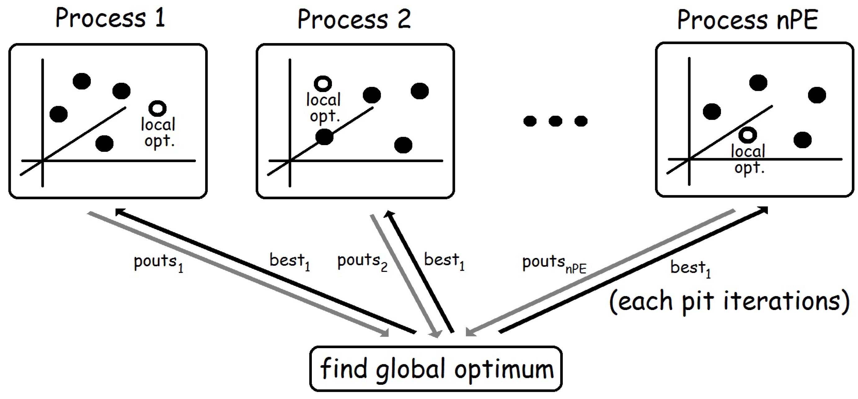
          psoPAR sg wpg np pit it nPE f bo = last bests
            where initPs = initialize sg np bo f
                  pass = unshuffle nPE initPs
                  sgs  = tail (generateSGs (nPE+1) sg)
                  pouts :: [ [(Double,Position)] ]
                  pouts = [process (psoP (sgs!!i) wpg pit f bo)#(pass!!i,bests1)
                             |i<-[0..nPE-1]] `using` spine
                  bests,bests1 :: [(Double,Position)]
                  bests  = map minimum (transp pouts)
                  bests1 = take it (obtainBest initPs : bests)
        

Figure 2. Basic structure of the second skeleton.

Figure 2. Basic structure of the second skeleton.

Let us remark that, in order to convert a sequential PSO algorithm into the corresponding parallel program, the programmer only has to change a call to function pso by a call to function psoPAR indicating appropriate values for parameters pit, it and nPE. In fact, the only programmer effort is due to selecting a reasonable value for pit.

Note that the programmer does not need to deal with the details of the parallelization. In fact, it is not even necessary that the programmer understands the details of the parallel implementation, provided that he understands the type interface of function psoPAR. Actually, the only function to be developed by the programmer is the fitness function. Moreover, it is important to recall that Eden programs can interact with other programming languages. In particular, C code can be encapsulated inside a Haskell function. Hence, Eden can be used as a coordination language dealing with the parallel structure of the program, whereas the core of the fitness function could be implemented in a computation language like C.

5.3. Alternative Skeletons

It is possible to provide more versions of the PSO skeleton so that the programmer can select the one that better fits his necessities. For instance, if the parallel environment to be used is not homogeneous, then the distribution of tasks among processors should take into account the characteristics of each processor. Let us consider a simple environment with two processors where one of them is much faster than the other. In that case, it would not be a good idea to assign half of the particles to each processor, because the faster one would finish its assignment in less time than the other one. Thus, it would be idle during the rest of the time, waiting until its counterpart finishes its tasks and thus reducing the overall performance of the system. Obviously, the problem is the same when the number of processors is larger and not all of them have the same speed.

The solution is simple: the number of tasks to be assigned to each processor should depend on the relative speed of all of them. Thus, instead of an integer denoting the number of available processors, the new skeleton has a new parameter containing a list of numbers denoting the speed of each processor. Note that, given the list, we also know the number of processors, so we can forget the nPE parameter. The type of the new skeleton is the following:

          psoPARh :: RandomGen a => a        --Random generator
                     -> WPGparams            --ω, ϕp and ϕr
                     -> Int                  --Number of particles
                     -> Int                  --Iterations per parallel step
                     -> Int                  --Number of parallel iterations
                     -> [Double]             --Speed of processors
                     -> (Position -> Double) --Fitness function
                     -> Boundaries           --Search space bounds
                     -> (Double,Position)    --Result: Best fitness and position
        

Regarding the implementation, we only need to modify the definition of psoPAR to include a new way to create the list of lists of particles pass by unshuffling the initial particles among processes, in such a way that their speeds are taken into account:

          psoPARh sg wpg np pit it speeds f bo = last bests
            where initPs = initialize sg np bo f
                  nPE = length speeds
                  pass = shuffleRelative speeds initPs
                  sgs  = tail (generateSGs (nPE+1) sg)
                  pouts :: [ [(Double,Position)] ]
                  pouts =[process (psoP (sgs!!i) wpg pit f bo) #(pass!!i,bests1)
                            |i<-[0..nPE-1]] `using` spine
                  bests,bests1 :: [(Double,Position)]
                  bests  = map minimum (transp pouts)
                  bests1 = take it (obtainBest initPs : bests)
       

The new function shuffleRelative first computes the percentage of tasks to be assigned to each process, and then it distributes the tasks by using function splitWith:

          shuffleRelative speeds tasks = splitWith percentages tasks
            where percentages=map (round.(m*).(/total)) speeds
                  total = sum speeds
                  m = fromIntegral (length tasks)
                  splitWith [n] xs = [xs]
                  splitWith (n:ns) xs = firsts:splitWith ns rest
                    where (firsts,rest) = splitAt n xs
        

Note that we do not need to change any other definition of the previous skeleton. In particular, the definition of process psoP is exactly the same.

Let us consider another alternative skeleton. In this case, we are interested in providing a version where the number of iterations to be performed in each parallel step is variable. Note that, during the first phases of the computation, the global optimum changes faster than during the last iterations. Thus, during the last phases we could use a larger number of independent parallel iterations, as the synchronization seems to be less important when the global optimum does not change significantly. In order to do that, we need to modify function psoPAR (or psoPARh) to change the previous parameters pit and it by a new parameter containing a list of integers. The first element of this list contains the number of iterations to be performed in parallel before the first global synchronization, the second element represents the number of parallel iterations before the second synchronization, and so on.

Note that this modification can be done in both the skeleton shown in the previous section and the new skeleton shown in this section, where the relative speed of processors is taken into account. We only show how to do it in the new skeleton, as the other one is modified analogously. The new type of function psoPARvh is the following:

          psoPARvh :: RandomGen a => a         --Random generator
                      -> WPGparams             --ω, ϕp and ϕr
                       -> Int                  --Number of particles
                       -> [Int]                --Iterations in each parallel step
                       -> [Double]             --Speed of processors
                       -> (Position -> Double) --Fitness function
                       -> Boundaries           --Search space bounds
                       -> (Double,Position)    --Result: Best fitness and position
       

and its new definition only has to appropriately compute the previous parameter it (number of global synchronizations) and pass the new list parameter pits to a new process psoPv:

          psoPARvh sg wpg np pits speeds f bo = last bests
            where ...
                  it = length pits
                  pouts=[process (psoPv (sgs!!i) wpg pits f bo)#(pass!!i,bests1)
                           |i<-[0..nPE-1]] `using` spine
                  ...
        

Regarding the new process psoPv, it is a very simple modification with respect to the previous process psoP. Now, instead of using always the same value pit as the number of iterations to be used by function pso’, in each step we take a new value pit from list pits:

          psoPv sg wpg (pit:pits) f bo (pas,newBest:newBests)
            = newOut : psoPv sg2 wpg pits f bo (newPas,newBests)
            where ...
                  newPas = pso’ rss wpg pit f bo pas’
                  ...
        

Note again that, once these skeletons are defined, the user does not need to know their internal definition in order to use them. It is only necessary to understand their external interface.

6. Experimental Results

In this section we present our experiments and report their results. In order to test the suitability of our PSO parallel approach, we develop the following methodology. First, we execute our PSO skeletons where the population of particles is split into islands. Particles within each island evolve independently and update their global optimum every n steps, as described in previous sections. This experiment allows us to study the effect of islands on the optimality of solutions. In order to perform this comparison, we use some known benchmark functions, in particular several functions studied in [39]. Second, after analyzing the influence of using islands, we analyze the speedup of our parallel schemes for the hardest problem considered in [39].

6.1. Experimental Setup

In our experiments, our implementations of PSO will be used to minimize the following functions, taken from [39]:

• Sphere Model: $f_1\left(x\right)={\sum }_{i=1}^n{x}_i^2$
• Schwefel’s Problem $2.22$: $f_2\left(x\right)={\sum }_{i=1}^n|x_i|+{\prod }_{i=1}^n\left|x_i\right|$
• Schwefel’s Problem $1.2$: $f_3\left(x\right)={\sum }_{i=1}^n{({\sum }_{j=1}^i{x}_j)}^2$
• Schwefel’s Problem $2.21$: $f_4\left(x\right)=ma{x}_i\left\{\right|x_i|,1\le i\le n\}$
• Generalized Rosenbrock’s Function: $f_5\left(x\right)={\sum }_{i=1}^{n-1}[100{(x_{i+1}-x_i^2)}^2+{(x_i-1)}^2]$
• Step Function: $f_6\left(x\right)={\sum }_{i=1}^n{\left(\lfloor x_i+0.5\rfloor \right)}^2$
• Generalized Schwefel’s Problem $2.26$: $f_8\left(x\right)={\sum }_{i=1}^n-x_{i}sin\left(\sqrt{|x_i|}\right)$
• Generalized Rastrigin’s Function: $f_9\left(x\right)={\sum }_{i=1}^n[x_i^2-10cos\left(2\pi x_i\right)+10]$
• Ackley’s Function: $f_{10}\left(x\right)=-20exp\left(-0.2\sqrt{\frac{1}{n}{\sum }_{i=1}^n{x}_i^2}\right)-exp\left(\frac{1}{n}{\sum }_{i=1}^{n}cos2\pi x_i\right)+20+e$
• Generalized Griewank Function: $f_{11}\left(x\right)=\frac{1}{4000}{\sum }_{i=1}^n{x}_i^2-{\prod }_{i=1}^{n}cos\left(\frac{x_i}{\sqrt{i}}\right)+1$
• Generalized Penalized Function I: $f_{12}\left(x\right)=\frac{\pi }{n}\left\{10{sin}^2\left(\pi y_i\right)+{\sum }_{i=1}^{n-1}{(y_i-1)}^2[1+10{sin}^2\left(\pi y_{i+1}\right)]+{(y_n-1)}^2\right\}+{\sum }_{i=1}^{n}u(x_i,10,100,4)$, $y_i=1+\frac{1}{4}(x_i+1)$, $u(x_i,a,k,m)=\left\{\begin{array}{cc}k{(x_i-a)}^m,\hfill & x_i>a\hfill \\ 0,\hfill & -a\le x_i\le a\hfill \\ k{(-x_i-a)}^m,\hfill & x_i<-a\hfill \end{array}\right.$
• Generalized Penalized Function II: $f_{13}\left(x\right)=0.1\left\{{sin}^2\left(3\pi x_1\right)+{\sum }_{i=1}^{n-1}{(x_i-1)}^2[1+{sin}^2\left(3\pi x_{i+1}\right)]+{(x_n-1)}^2[1+si{n}^2\left(2\pi x_n\right)]\right\}+{\sum }_{i=1}^{n}u(x_i,5,100,4)$
• Shekel’s Foxholes Function: $f_{14}\left(x\right)=\left[\frac{1}{500}+{\sum }_{j=1}^{25}\frac{1}{j+{\sum }_{i=1}^2{(x_i-a_{ij})}^6}\right]$
• Kowalik’s Function: $f_{15}\left(x\right)={\sum }_{i=1}^{11}{\left[a_i-\frac{x_1(b_i^2+b_i{x}_2)}{b_i^2+b_i{x}_3+x_4}\right]}^2$
• Six-Hump Camel-Back Function: $f_{16}\left(x\right)=4x_1^2-2.1x_1^4+\frac{1}{3}{x}_1^6+x_1{x}_2-4x_2^2+4x_2^4$
• Branin Function: $f_{17}\left(x\right)={\left(x_2-\frac{5.1}{4{\pi }^2}{x}_1^2+\frac{5}{\pi }{x}_1-6\right)}^2+10\left(1-\frac{1}{8\pi }\right)cos{x}_1+10$

The most relevant features of these functions are depicted in Table 1. For each function, we show the number of dimensions, the boundaries of the solutions space, the value of the optimal solution, and the asymmetric initialization range used in the experiments. The first six functions are relatively simple, whereas finding the minimum value of functions $f_8-f_{13}$ is harder. The reason is that there are more local minima in these functions. In fact, the number of local minima is exponential with respect to the number of dimensions of these problems. Functions $f_{14}-f_{17}$ are low-dimensional functions which have only a few local minima.

Table 1. Benchmark functions.

Function	Dimensions (n)	${[\mathit{min},\mathit{max}]}^n$	$f{\left(x\right)}_{\mathit{min}}$	Asym. Init. Range
$f_1\left(x\right)$	30	${[-100,100]}^n$	0	${[-100,-33.3]}^n$
$f_2\left(x\right)$	30	${[-10,10]}^n$	0	${[-10,-3.3]}^n$
$f_3\left(x\right)$	30	${[-100,100]}^n$	0	${[-100,-33.3]}^n$
$f_4\left(x\right)$	30	${[-100,100]}^n$	0	${[-100,-33.3]}^n$
$f_5\left(x\right)$	30	${[-30,30]}^n$	0	${[-30,-10]}^n$
$f_6\left(x\right)$	30	${[-100,100]}^n$	0	${[-100,-33.3]}^n$
$f_8\left(x\right)$	30	${[-500,500]}^n$	$-12569.5$	${[-500,500]}^n$
$f_9\left(x\right)$	30	${[-5.12,5.12]}^n$	0	${[-5.12,-1.7]}^n$
$f_{10}\left(x\right)$	30	${[-32,32]}^n$	0	${[-32,-10.7]}^n$
$f_{11}\left(x\right)$	30	${[-600,600]}^n$	0	${[-600,-200]}^n$
$f_{12}\left(x\right)$	30	${[-50,50]}^n$	0	${[-50,-16.7]}^n$
$f_{13}\left(x\right)$	30	${[-50,50]}^n$	0	${[-50,-16.7]}^n$
$f_{14}\left(x\right)$	2	${[-65.536,65.536]}^n$	1	${[-65.536,-21.84]}^n$
$f_{15}\left(x\right)$	4	${[-5,5]}^n$	0.0003075	${[-5,-1.67]}^n$
$f_{16}\left(x\right)$	2	${[-5,5]}^n$	−1.0316285	${[-5,-1.67]}^n$
$f_{17}\left(x\right)$	2	$[-\mathrm{5,10}]\times \left[\mathrm{0,15}\right]$	0.398	$[-5,-1.67]\times \left[\mathrm{0,5}\right]$

Table 1. Benchmark functions.

Function	Dimensions (n)	${[\mathit{min},\mathit{max}]}^n$	$f{\left(x\right)}_{\mathit{min}}$	Asym. Init. Range
$f_1\left(x\right)$	30	${[-100,100]}^n$	0	${[-100,-33.3]}^n$
$f_2\left(x\right)$	30	${[-10,10]}^n$	0	${[-10,-3.3]}^n$
$f_3\left(x\right)$	30	${[-100,100]}^n$	0	${[-100,-33.3]}^n$
$f_4\left(x\right)$	30	${[-100,100]}^n$	0	${[-100,-33.3]}^n$
$f_5\left(x\right)$	30	${[-30,30]}^n$	0	${[-30,-10]}^n$
$f_6\left(x\right)$	30	${[-100,100]}^n$	0	${[-100,-33.3]}^n$
$f_8\left(x\right)$	30	${[-500,500]}^n$	$-12569.5$	${[-500,500]}^n$
$f_9\left(x\right)$	30	${[-5.12,5.12]}^n$	0	${[-5.12,-1.7]}^n$
$f_{10}\left(x\right)$	30	${[-32,32]}^n$	0	${[-32,-10.7]}^n$
$f_{11}\left(x\right)$	30	${[-600,600]}^n$	0	${[-600,-200]}^n$
$f_{12}\left(x\right)$	30	${[-50,50]}^n$	0	${[-50,-16.7]}^n$
$f_{13}\left(x\right)$	30	${[-50,50]}^n$	0	${[-50,-16.7]}^n$
$f_{14}\left(x\right)$	2	${[-65.536,65.536]}^n$	1	${[-65.536,-21.84]}^n$
$f_{15}\left(x\right)$	4	${[-5,5]}^n$	0.0003075	${[-5,-1.67]}^n$
$f_{16}\left(x\right)$	2	${[-5,5]}^n$	−1.0316285	${[-5,-1.67]}^n$
$f_{17}\left(x\right)$	2	$[-\mathrm{5,10}]\times \left[\mathrm{0,15}\right]$	0.398	$[-5,-1.67]\times \left[\mathrm{0,5}\right]$

In our experiments, values ω, $\varphi p$, and $\varphi r$ are set as proposed in [29]. For each function, the number of iterations is the same as the number of algorithm iterations performed in [39], while the number of particles is 100. Following the asymmetric initialization approach given in [40], particles are asymmetrically distributed for all problems but $f_8$, which is appointed as specially hard for using an asymmetric initialization in that work. In this special case we use an homogeneous distribution, as it is done in [40].

6.2. Analyzing the Influence of Using Islands

We start studying the effect on the quality of solutins of using islands. Note that splitting particles into sets which independently evolve and update the global optimum only from time to time has two effects. On the one hand, enabling such an independent evolution of particles helps to preserve the diversity of solutions. On the other hand, out-of-date global optima may prevent particles from searching for solutions in more interesting areas for a while, until the global optimum is updated again. In order to obtain results that are statistically relevant, for each function and number of islands, we perform 50 executions and we compute the corresponding averages. In Table 2 we depict the results of our PSO skeleton for 1, 2, 3, and 4 islands (note that using 1 island is the same as not considering islands at all).

Table 2. Average optimality comparison with different number of islands.

Function	1 Island	2 Islands	3 Islands	4 Islands
$f_1\left(x\right)$	$1.02\times {10}^{-4}$	$2.91\times {10}^{-4}$	$9.54\times {10}^{-4}$	$1.22\times {10}^{-3}$
$f_2\left(x\right)$	$8.29\times {10}^{-3}$	$1.15\times {10}^{-2}$	$1.18\times {10}^{-2}$	$1.47\times {10}^{-2}$
$f_3\left(x\right)$	$1.93\times {10}^{-5}$	$5.40\times {10}^{-5}$	$6.55\times {10}^{-5}$	$1.57\times {10}^{-4}$
$f_4\left(x\right)$	$1.45\times {10}^{-3}$	$1.69\times {10}^{-3}$	$1.57\times {10}^{-3}$	$1.60\times {10}^{-3}$
$f_5\left(x\right)$	$26.57$	$8.56$	$12.96$	$14.01$
$f_6\left(x\right)$	0	0	0	0
$f_8\left(x\right)$	$-9686.99$	$-9699.22$	$-9892.67$	$-\mathrm{10,126.50}$
$f_9\left(x\right)$	$6.97\times {10}^{-8}$	$2.28\times {10}^{-7}$	$1.19\times {10}^{-6}$	$2.04\times {10}^{-6}$
$f_{10}\left(x\right)$	$2.41\times {10}^{-3}$	$3.98\times {10}^{-3}$	$3.98\times {10}^{-3}$	$6.65\times {10}^{-3}$
$f_{11}\left(x\right)$	$4.69\times {10}^{-3}$	$5.59\times {10}^{-3}$	$5.88\times {10}^{-3}$	$5.86\times {10}^{-3}$
$f_{12}\left(x\right)$	$6.33\times {10}^{-3}$	$2.52\times {10}^{-4}$	$5.05\times {10}^{-4}$	$8.24\times {10}^{-4}$
$f_{13}\left(x\right)$	$0.04$	$0.05$	$0.04$	$0.06$
$f_{14}\left(x\right)$	$1.65$	$1.69$	$1.41$	$1.48$
$f_{15}\left(x\right)$	$1.22\times {10}^{-3}$	$1.20\times {10}^{-3}$	$1.22\times {10}^{-3}$	$1.20\times {10}^{-3}$
$f_{16}\left(x\right)$	$-1.03$	$-1.03$	$-1.03$	$-1.03$
$f_{17}\left(x\right)$	$0.398$	$0.398$	$0.398$	$0.398$

Table 2. Average optimality comparison with different number of islands.

Function	1 Island	2 Islands	3 Islands	4 Islands
$f_1\left(x\right)$	$1.02\times {10}^{-4}$	$2.91\times {10}^{-4}$	$9.54\times {10}^{-4}$	$1.22\times {10}^{-3}$
$f_2\left(x\right)$	$8.29\times {10}^{-3}$	$1.15\times {10}^{-2}$	$1.18\times {10}^{-2}$	$1.47\times {10}^{-2}$
$f_3\left(x\right)$	$1.93\times {10}^{-5}$	$5.40\times {10}^{-5}$	$6.55\times {10}^{-5}$	$1.57\times {10}^{-4}$
$f_4\left(x\right)$	$1.45\times {10}^{-3}$	$1.69\times {10}^{-3}$	$1.57\times {10}^{-3}$	$1.60\times {10}^{-3}$
$f_5\left(x\right)$	$26.57$	$8.56$	$12.96$	$14.01$
$f_6\left(x\right)$	0	0	0	0
$f_8\left(x\right)$	$-9686.99$	$-9699.22$	$-9892.67$	$-\mathrm{10,126.50}$
$f_9\left(x\right)$	$6.97\times {10}^{-8}$	$2.28\times {10}^{-7}$	$1.19\times {10}^{-6}$	$2.04\times {10}^{-6}$
$f_{10}\left(x\right)$	$2.41\times {10}^{-3}$	$3.98\times {10}^{-3}$	$3.98\times {10}^{-3}$	$6.65\times {10}^{-3}$
$f_{11}\left(x\right)$	$4.69\times {10}^{-3}$	$5.59\times {10}^{-3}$	$5.88\times {10}^{-3}$	$5.86\times {10}^{-3}$
$f_{12}\left(x\right)$	$6.33\times {10}^{-3}$	$2.52\times {10}^{-4}$	$5.05\times {10}^{-4}$	$8.24\times {10}^{-4}$
$f_{13}\left(x\right)$	$0.04$	$0.05$	$0.04$	$0.06$
$f_{14}\left(x\right)$	$1.65$	$1.69$	$1.41$	$1.48$
$f_{15}\left(x\right)$	$1.22\times {10}^{-3}$	$1.20\times {10}^{-3}$	$1.22\times {10}^{-3}$	$1.20\times {10}^{-3}$
$f_{16}\left(x\right)$	$-1.03$	$-1.03$	$-1.03$	$-1.03$
$f_{17}\left(x\right)$	$0.398$	$0.398$	$0.398$	$0.398$

In order to statistically analyze the influence of using islands on the optimality of the solutions, we use [41] to perform a statistical test of the mean results given in Table 2. In general, a Friedman test [42,43] can be used to check whether the hypothesis that all methods behave similarly (the null hypothesis) holds or not. However, since the number of variables (methods) under consideration is low, using a Friedman aligned ranks test [44] or a Quade test [45] is more recommended in this case (see e.g., [46]). These tests do not rank methods for each problem separately (as Friedman test does), but construct a global ranking where values of all methods and problems are ranked together. In Friedman aligned ranks test, for each problem the difference of each method with respect to the average value for all methods is considered, and next all values of all problems are ranked together. In Quade test, problems where the difference between the best result and the worst result is high are given more weight in the comparison. Let us consider $\alpha =0.05$, a standard significance level. From results given in Table 2, we calculate that the p-value for aligned Friedman is 0.0049, which allows to reject the null hypothesis with a high level of significance (the p-value is much lower than 0.05). So, the test concludes that methods using 1, 2, 3 and 4 islands are not considered similar. That is, algorithms using different numbers of islands are not considered equivalent. Since the null hypothesis was rejected, we can apply a post-hoc analysis to compare the control method with the other three. Ranks assigned by this test to these methods are 33.1563, 33.8750, 28.3438 and 34.6250, respectively. Thus, the control method consists in using 3 islands. The p-values of the comparison of the 3-island method with respect to 4, 2, and 1 islands respectively are 0.3400, 0.4008, 0.4647 respectively, and Holm’s procedure requires that these values are iteratively lower than 0.0167, 0.0250 and 0.0500, respectively. Since the condition does not hold for the first comparison, the three null hypotheses are accepted, so all methods with 4, 2, and 1 islands are pairwise considered equivalent to using 3 islands. Note that, although we cannot find relevant differences when comparing them pairwise, when we consider the four methods together the differences are found by the test.

Now we consider the Quade test. This time the p-value is 0.0228, so the test concludes that using 1, 2, 3 or 4 islands is not (globally) equivalent. The ranks given by Quade test to these methods are 2.3125, 2.4522, 2.3346 and 2.9007, respectively. Thus, the control method is 1 island. The p-values of the comparison of 1 island with 4, 3, and 2 islands are 0.3550, 0.8261 and 0.9723, and Holm’s procedure requires that these values are lower than 0.0167, 0.0250 and 0.0500, respectively. Again, the first comparison fails, so all null hypotheses are accepted. Thus, methods with 4, 3 and 2 islands are pairwise considered equivalent to using 1 island.

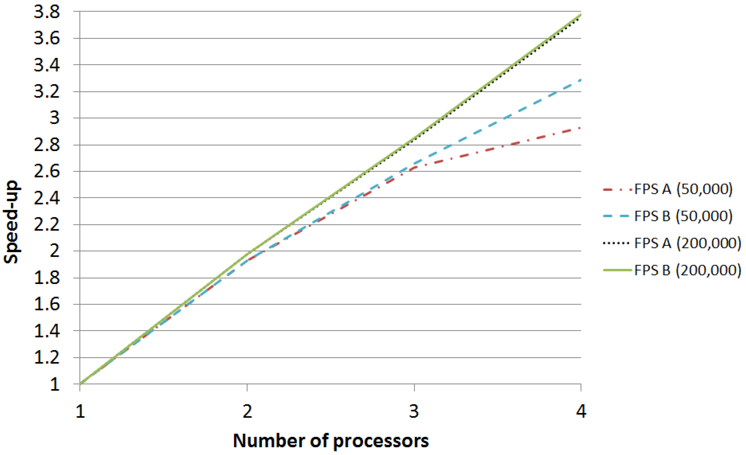
6.3. Speedup Analysis

Let us note that, after executing our PSO skeletons for the same number of iterations as those used in [39], there is still margin for improving results further, specially for the hardest problem ($f_8$). In Table 3 we depict results for $f_8$ for higher numbers of iterations. They illustrate that better solutions are found after iteration 9000 indeed.

Table 3. Solutions found with different number of iterations.

Function	Iterations	Best Sol	Arith Mean	Std Dev
$f_8\left(x\right)$	9000	$-\mathrm{12,095.73}$	$-9686.99$	$1362.44$
$f_8\left(x\right)$	$\mathrm{50,000}$	$-\mathrm{12,214.17}$	$-\mathrm{10,339.49}$	$1062.38$
$f_8\left(x\right)$	$\mathrm{200,000}$	$-\mathrm{12,569.48}$	$-\mathrm{11,091.23}$	$1011.68$

Table 3. Solutions found with different number of iterations.

Function	Iterations	Best Sol	Arith Mean	Std Dev
$f_8\left(x\right)$	9000	$-\mathrm{12,095.73}$	$-9686.99$	$1362.44$
$f_8\left(x\right)$	$\mathrm{50,000}$	$-\mathrm{12,214.17}$	$-\mathrm{10,339.49}$	$1062.38$
$f_8\left(x\right)$	$\mathrm{200,000}$	$-\mathrm{12,569.48}$	$-\mathrm{11,091.23}$	$1011.68$

Next we present the speedups obtained by using our skeletons. In order to analyze their parallel performance, we use two computers which are connected through the intranet of our university and are physically located in different buildings. Both computers use the same Linux distribution (Debian), the same MPI library (OpenMPI 1.4.2), and have analogous Intel Core i3 Duo processors. Thus, we perform parallel experiments with up to four cores.

Among the 16 problems presented in our previous experiments, we select the hardest one ($f_8$) because it requires the longest execution time to obtain good solutions. Thus, it is more likely to improve its time performance by taking advantage of a parallel execution. We conducted two experiments. In the first one, algorithms are run for 50,000 iterations, and in the second they are executed for 200,000 iterations. For each case, we use two different skeletons: the one presented in Section 5.2 (FPS A, standing for Functional Particle Swarm), and the final modified version presented in Section 5.3 (FPS B). Since the parallel environment is homogeneous, trying to take advantage of the first skeleton implemented in Section 5.3 to compensate different processors speed would not provide any advantage in this case. In experiments with 50,000 iterations, FPS A updates the global optimum every 500 iterations and does so 100 times, whereas FPS B updates the global optimum every 500 steps for the first 10 times, and next it updates it every 5000 iterations 9 times. In experiments with 200,000 iterations, FPS A updates the optimum every 5000 iterations and does it 40 times, whereas FPS B updates the global optimum every 5000 steps for the first 10 times, and next it updates it every 50,000 steps 3 times.

Each parallel skeleton is executed for up to four processors, and the speedup is computed by comparing its execution time with the time of the sequential version. Table 4 summarizes the execution time (in seconds) and the speedup obtained for each input problem and for each skeleton. As it can be expected, FPS B obtains better results than FPS A, as it reduces the communications among processes. The difference between both skeletons is small in the case of the largest execution ($3.78$ vs. $3.76$ speedup with 4 processors), but it is more significant in the case of the shortest one ($3.29$ vs. $2.93$). The reason is that the impact of communications in the largest execution is already small in FPS A, so there is small room for improvement for FPS B. However, in the case of the shortest execution, communications take place more often (in relative terms) so their impact is higher. The speedup of experiments is graphically compared in Figure 3.

Table 4. Times and speedups comparison.

Version	Iterations	Processors	Time	Speedup
FPS	$\mathrm{50,000}$	1	$113.45$	1
FPS A	$\mathrm{50,000}$	2	$58.73$	$1.93$
FPS B	$\mathrm{50,000}$	2	$58.71$	$1.93$
FPS A	$\mathrm{50,000}$	3	$43.13$	$2.63$
FPS B	$\mathrm{50,000}$	3	$42.66$	$2.66$
FPS A	$\mathrm{50,000}$	4	$38.69$	$2.93$
FPS B	$\mathrm{50,000}$	4	$34.50$	$3.29$
FPS	$\mathrm{200,000}$	1	$429.17$	1
FPS A	$\mathrm{200,000}$	2	$216.96$	$1.98$
FPS B	$\mathrm{200,000}$	2	$216.30$	$1.98$
FPS A	$\mathrm{200,000}$	3	$151.26$	$2.84$
FPS B	$\mathrm{200,000}$	3	$150.79$	$2.85$
FPS A	$\mathrm{200,000}$	4	$114.21$	$3.76$
FPS B	$\mathrm{200,000}$	4	$113.56$	$3.78$

Table 4. Times and speedups comparison.

Version	Iterations	Processors	Time	Speedup
FPS	$\mathrm{50,000}$	1	$113.45$	1
FPS A	$\mathrm{50,000}$	2	$58.73$	$1.93$
FPS B	$\mathrm{50,000}$	2	$58.71$	$1.93$
FPS A	$\mathrm{50,000}$	3	$43.13$	$2.63$
FPS B	$\mathrm{50,000}$	3	$42.66$	$2.66$
FPS A	$\mathrm{50,000}$	4	$38.69$	$2.93$
FPS B	$\mathrm{50,000}$	4	$34.50$	$3.29$
FPS	$\mathrm{200,000}$	1	$429.17$	1
FPS A	$\mathrm{200,000}$	2	$216.96$	$1.98$
FPS B	$\mathrm{200,000}$	2	$216.30$	$1.98$
FPS A	$\mathrm{200,000}$	3	$151.26$	$2.84$
FPS B	$\mathrm{200,000}$	3	$150.79$	$2.85$
FPS A	$\mathrm{200,000}$	4	$114.21$	$3.76$
FPS B	$\mathrm{200,000}$	4	$113.56$	$3.78$

Figure 3. Speedup comparison.

Figure 3. Speedup comparison.

Let us remark that, once the skeletons were written, the programming effort needed to use them was negligible. We only needed to decide the number of iterations to be performed in parallel before each global synchronization. However, observed speedups (specially for FPS B) are satisfactory.

7. Conclusions and Future Work

We have shown how to use the parallel functional language Eden to provide parallel versions of PSO algorithms by means of Eden skeletons. The programmer only has to provide an appropriate fitness function and adjust parameters, whereas all low-level details of the parallelization are done automatically by the skeleton and the underlying runtime system. Moreover, different parallel implementations of PSO can be provided to the user (in the paper we have shown four of them) so that he can select the one that better fits his necessities.

It is worth pointing out that the source code used to develop the skeletons is highly reusable. First, any programmer can use it by just defining an appropriate fitness function, while the whole parallel machinery is done automatically by the provided skeleton. Second, it is simple to modify the skeleton to obtain alternative parallel versions of it. In particular, we have shown how to modify psoPAR to obtain a different version called psoPARh to deal with heterogeneous processors, and we have also shown how to modify such version to obtain another version psoPARhv where the number of iterations to be performed in each parallel step is variable. In both cases, it was only necessary to modify a couple of lines of the source code to obtain the alternative version, keeping unmodified the main part of the source code.

Our experiments have shown that the programmer does not need much work to adjust a skeleton to his concrete problem, but achieved speedups are good enough. Note that we do not claim to obtain optimal speedups but reasonable speedups—at low programmer effort.

In our previous work [31], we showed how to use Eden skeletons to deal with the parallelization of genetic algorithms. In fact, our aim is to provide a library of generic Haskell versions of the most common bioinspired metaheuristics, as well as a library containing the corresponding Eden skeletons for each metaheuristic. By doing so, we will simplify the task of using these metaheuristics in functional settings, and we will also simplify the task of improving their performance by means of parallelizing them. Moreover, as several metaheuristics will be provided in the same environment, the programmer will be able to check more easily what metaheuristics fits better for each concrete problem.

In addition to extending our library to deal with other swarm metaheuristics (like Ant Colony Optimization or River Formation Dynamics), as future work we are particularly interested in studying hybrid systems combining different metaheuristics.

References

1. Eiben, A.; Smith, J. Introduction to Evolutionary Computing; Springer: Heidelberg, Germany, 2003. [Google Scholar]
2. Chiong, R. Nature-Inspired Algorithms for Optimisation; Chiong, R., Ed.; Springer: Heidelberg, Germany, 2009; Volume 193. [Google Scholar]
3. Kennedy, J.; Eberhart, R. Swarm Intelligence; The Morgan Kaufmann Publishers: San Francisco, USA, 2001. [Google Scholar]
4. Kennedy, J. Swarm Intelligence. In Handbook of Nature-Inspired and Innovative Computing; Zomaya, A., Ed.; Springer: New York, USA, 2006; pp. 187–219. [Google Scholar]
5. Dorigo, M.; Maniezzo, V.; Colorni, A. Ant system: Optimization by a colony of cooperating agents. IEEE Trans. Syst. Man Cybern. Part B 1996, 26, 29–41. [Google Scholar] [CrossRef] [PubMed]
6. Rabanal, P.; Rodríguez, I.; Rubio, F. Using River Formation Dynamics to Design Heuristic Algorithms. In Unconventional Computation, Proceedings of the 6th International Conference, UC 2007, Kingston, ON, Canada, 13–17 Augurst 2007; Springer: Heidelberg, Germany, 2007; pp. 163–177. [Google Scholar]
7. Civicioglu, P.; Besdok, E. A conceptual comparison of the Cuckoo-search, particle swarm optimization, differential evolution and artificial bee colony algorithms. Artif. Intell. Rev. 2013, 39, 315–346. [Google Scholar] [CrossRef]
8. Cantú-Paz, E. A Survey of Parallel Genetic Algorithms. Calc. Parall. Reseaux Syst. Repartis 1998, 10, 141–171. [Google Scholar]
9. Alba, E. Parallel evolutionary algorithms can achieve super-linear performance. Inf. Process. Lett. 2002, 82, 7–13. [Google Scholar] [CrossRef]
10. Randall, M.; Lewis, A. A Parallel Implementation of Ant Colony Optimization. J. Parallel Distrib. Comput. 2002, 62, 1421–1432. [Google Scholar] [CrossRef]
11. Nedjah, N.; de Macedo-Mourelle, L.; Alba, E. Parallel Evolutionary Computations; Nedjah, N., de Macedo-Mourelle, L., Alba, E., Eds.; Studies in Computational Intelligence, Springer: Heidelberg, Germany, 2006; Volume 22. [Google Scholar]
12. Zhou, Y.; Tan, Y. GPU-based parallel particle swarm optimization. In Proceedings of the Eleventh Conference on Congress on Evolutionary Computation, Trondheim, Norway, 18–21 May 2009; IEEE Press: Piscataway, USA, 2009; pp. 1493–1500. [Google Scholar]
13. Mussi, L.; Daolio, F.; Cagnoni, S. Evaluation of parallel particle swarm optimization algorithms within the CUDA (TM) architecture. Inf. Sci. 2011, 181, 4642–4657. [Google Scholar] [CrossRef]
14. Achten, P.; van Eekelen, M.; Koopman, P.; Morazán, M. Trends in Trends in Functional Programming 1999/2000 versus 2007/2008. High.-Order Symb. Comput. 2010, 23, 465–487. [Google Scholar] [CrossRef]
15. Cole, M. Bringing Skeletons out of the Closet: A Pragmatic Manifesto for Skeletal Parallel Programming. Parallel Comput. 2004, 30, 389–406. [Google Scholar] [CrossRef]
16. Trinder, P.W.; Hammond, K.; Loidl, H.W.; Peyton Jones, S.L. Algorithm + Strategy = Parallelism. J. Funct. Programm. 1998, 8, 23–60. [Google Scholar] [CrossRef]
17. Klusik, U.; Loogen, R.; Priebe, S.; Rubio, F. Implementation Skeletons in Eden: Low-Effort Parallel Programming. In Proceedings of the 12th International Workshop on the Implementation of Functional Languages, IFL 2000, Aachen, Germany, 4–7 September 2000; Springer: Heidelberg, Germany, 2001; pp. 71–88. [Google Scholar]
18. Scaife, N.; Horiguchi, S.; Michaelson, G.; Bristow, P. A Parallel SML Compiler Based on Algorithmic Skeletons. J. Funct. Programm. 2005, 15, 615–650. [Google Scholar] [CrossRef]
19. Marlow, S.; Peyton Jones, S.L.; Singh, S. Runtime Support for Multicore Haskell. In Proceedings of the International Conference on Functional Programming, ICFP’09, Edinburgh, Scotland, 31 August–2 September 2009; pp. 65–78.
20. Keller, G.; Chakravarty, M.; Leshchinskiy, R.; Peyton Jones, S.; Lippmeier, B. Regular, shape-polymorphic, parallel arrays in Haskell. In Proceedings of the International Conference on Functional Programming (ICFP’10), Baltimore, Maryland, 27–29 September 2010; pp. 261–272.
21. Marlow, S. Parallel and Concurrent Programming in Haskell: Techniques for Multicore and Multithreaded Programming; O’Reilly Media, Inc.: Sebastopol, USA, 2013. [Google Scholar]
22. Loogen, R.; Ortega-Mallén, Y.; Peña, R.; Priebe, S.; Rubio, F. Parallelism Abstractions in Eden. In Patterns and Skeletons for Parallel and Distributed Computing; Rabhi, F.A., Gorlatch, S., Eds.; Springer: London, UK, 2002; pp. 95–128. [Google Scholar]
23. Peyton Jones, S.L.; Hughes, J. Report on the Programming Language Haskell 98. Technical report, Microsoft Research (Cambridge) and Chalmers University of Technology, 1999. Available online: http://www.haskell.org (accessed on 22 October 2014).
24. Kennedy, J.; Eberhart, R. Particle Swarm Optimization. In Proceedings of the IEEE International Conference on Neural Networks; IEEE Computer Society Press: Piscataway, USA, 1995; Volume 4, pp. 1942–1948. [Google Scholar]
25. Shi, Y.; Eberhart, R. A modified particle swarm optimizer. In Proceedings of the IEEE International Conference on Evolutionary Computation; IEEE Computer Society Press: Piscataway, USA, 1998; pp. 69–73. [Google Scholar]
26. Clerc, M.; Kennedy, J. The particle swarm—Explosion, stability, and convergence in a multidimensional complex space. IEEE Trans. Evolut. Comput. 2002, 6, 58–73. [Google Scholar] [CrossRef]
27. Parsopoulos, K.; Vrahatis, M. Recent approaches to global optimization problems through Particle Swarm Optimization. Nat. Comput. 2002, 1, 235–306. [Google Scholar] [CrossRef]
28. Zhan, Z.H.; Zhang, J.; Li, Y.; Chung, H.H. Adaptive Particle Swarm Optimization. IEEE Trans. Syst. Man Cybern. 2009, 39, 1362–1381. [Google Scholar] [CrossRef] [PubMed]
29. Pedersen, M. Tuning & Simplifying Heuristical Optimization. PhD Thesis, University of Southampton, Southampton, UK, 2010. [Google Scholar]
30. Abido, M. Multiobjective particle swarm optimization with nondominated local and global sets. Nat. Comput. 2010, 9, 747–766. [Google Scholar] [CrossRef]
31. Encina, A.V.; Hidalgo-Herrero, M.; Rabanal, P.; Rubio, F. A Parallel Skeleton for Genetic Algorithms. In Proceedings of the International Work-Conference on Artificial Neural Networks, IWANN 2011; Springer: Heidelberg, 2011; pp. 388–395. [Google Scholar]
32. Goldberg, D. Genetic Algorithms in Search, Optimisation and Machine Learning; Addison-Wesley: Boston, USA, 1989. [Google Scholar]
33. Hidalgo-Herrero, M.; Ortega-Mallén, Y.; Rubio, F. Analyzing the influence of mixed evaluation on the performance of Eden skeletons. Parallel Comput. 2006, 32, 523–538. [Google Scholar] [CrossRef]
34. Eberhart, R.; Simpson, P.; Dobbins, R. Computational Intelligence PC Tools; Academic Press Professional: San Diego, USA, 1996. [Google Scholar]
35. Kennedy, J. Small worlds and mega-minds: Effects of neighborhood topology on particle swarm performance. In Congress on Evolutionary Computation; IEEE Computer Society Press: Piscataway, USA, 1999; Volume 3, pp. 1931–1938. [Google Scholar]
36. Shi, Y.; Eberhart, R. Parameter Selection in Particle Swarm Optimization. In Evolutionary Programming; LNCS; Springer: Heidelberg, Germany, 1998; Voloume1447, pp. 591–600. [Google Scholar]
37. Beielstein, T.; Parsopoulos, K.; Vrahatis, M. Tuning PSO parameters through sensitivity analysis. Technical report. Universität Dortmund: Germany, 2002. [Google Scholar]
38. Laskari, E.C.; Parsopoulos, K.E.; Vrahatis, M.N. Particle Swarm Optimization for Integer Programming. In IEEE Congress on Evolutionary Computation; IEEE Computer Society Press: Piscataway, USA, 2002; pp. 1576–1581. [Google Scholar]
39. Yao, X.; Liu, Y.; Lin, G. Evolutionary programming made faster. IEEE Trans. Evolut. Comput. 1999, 3, 82–102. [Google Scholar]
40. Worasucheep, C. A particle swarm optimization for high-dimensional function optimization. In Proceedings of the International Conference on Electrical Engineering/Electronics Computer Telecommunications and Information Technology (ECTI-CON’10); IEEE Computer Society Press: Piscataway, USA, 2010; pp. 1045–1049. [Google Scholar]
41. Parejo-Maestre, J.; García-Gutiérrez, J.; Ruiz-Cortés, A.; Riquelme-Santos, J. STATService. Available online: http://moses.us.es/statservice/ (accessed on 22 October 2014).
42. Friedman, M. The use of ranks to avoid the assumption of normality implicit in the analysis of variance. J. Am. Stat. Assoc. 1937, 32, 674–701. [Google Scholar] [CrossRef]
43. Friedman, M. A comparison of alternative tests of significance for the problem of m rankings. Ann. Math. Stat. 1940, 11, 86–92. [Google Scholar] [CrossRef]
44. Hodges, J.; Lehmann, E. Ranks methods for combination of independent experiments in analysis of variance. Ann. Math. Stat. 1962, 33, 482–497. [Google Scholar] [CrossRef]
45. Quade, D. Using weighted rankings in the analysis of complete blocks with additive block effects. J. Am. Stat. Assoc. 1979, 74, 680–683. [Google Scholar] [CrossRef]
46. Derrac, J.; García, S.; Molina, D.; Herrera, F. A practical tutorial on the use of nonparametric statistical tests as a methodology for comparing evolutionary and swarm intelligence algorithms. Swarm Evol. Comput. 2011, 1, 3–18. [Google Scholar] [CrossRef]